A Work Project, presented as part of the requirements for the Award of a Master’s degree in Finance from the Nova School of Business and Economics.
CORPORATE BANKRUPTCY PREDICTION: A COMPARISON OF LOGISTIC REGRESSION AND RANDOM FOREST ON PORTUGUESE COMPANY DATA
SINA BRUHN – 33996
Work Project carried out under the supervision of: Ricardo João Gil Pereira
Abstract
In the current field of bankruptcy prediction studies, the geographical focus usually is on larger economies rather than economies the size of Portugal. For the purpose of this study financial statement data from five consecutive years prior to the event of bankruptcy in 2017 was selected. Within the data 328,542 healthy and unhealthy Portuguese companies were included. Two predictive models using the Logistic Regression and Random Forest algorithm were fitted to be able to predict bankruptcy. Both developed models deliver good results even though the Random Forest model performs slightly better than the one based on Logistic Regression.
Keywords
Bankruptcy prediction, Logistic Regression, Random Forest, Portugal
This work used infrastructure and resources funded by Fundação para a Ciência e a Tecnologia (UID/ECO/00124/2013, UID/ECO/00124/2019 and Social Sciences DataLab, Project 22209), POR Lisboa (LISBOA-01-0145-FEDER-007722 and Social Sciences DataLab, Project 22209) and POR Norte (Social Sciences DataLab, Project 22209).
I Contents List of figures ... II List of tables ... II 1. Introduction ... 1 2. Literature review ... 2 3. Data ... 4 4. Research methodology ... 9
5. Results and discussion ... 12
6. Conclusion ... 17 References ... XVIII Appendices ... XXII
II List of figures
Figure 1: Extract from the dataset 6
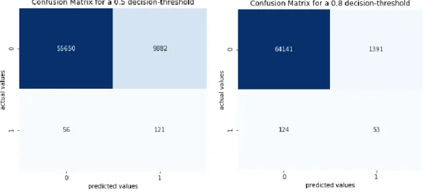
Figure 2: ROC Curve of Logistic Regression and Random Forest classifier 14 Figure A1: Visualization of the data before and after the transformation process XXIII Figure A2: Confusion Matrices of the Logistic Regression classifier for different decision
thresholds XXIV
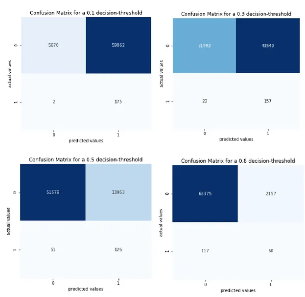
Figure A3: Confusion Matrices of the Random Forest classifier for different decision
thresholds XXIV
List of tables
Table 1: Results 12
Table A1: Variables used as underlying data XXII
Table A2: Statistics of the underlying data before and after the transformation process XXII Table A3: Top 5 and bottom 5 coefficients of the Logistic Regression classifier XXIII Table A4: Top 10 features by importance of the Random Forest classifier XXIII
1 1. Introduction
Although numerous studies concerning bankruptcy prediction have been conducted all over the world, they still remain a topic of interest (Ziȩba et al, 2016). The ability to gauge companies accurately and classify them ahead of time correctly is crucial, since the bankruptcy of a company does not only affect its image and ongoing business but also its employees as well as other stakeholders (Geng et al, 2015). Banks have an inherent interest of knowing ahead of time whether a corporate client has a high chance of filing for bankruptcy, since they might need to adjust credit lines or interest rates for existing loans. Also, suppliers are interested in the financial health of their business counterparts. They might end the business relationship altogether, reduce the supply volume or change the payment conditions in order to decrease their exposure to potentially defaulting parties (Krommes, 2011).
So far, the research has not centered on Portuguese company data often. There are just a few studies like Moody’s KMV Risk Calc model (Dwyer et al, 2004) or specific paper concentrating on the textile industry (Leal et al, 2007) which focus on bankruptcy prediction for Portuguese companies. In addition, Portugal is of special interest because of its intriguing economic development and the heavy influence of the financial crisis.
Therefore, this paper’s concentration is on Portuguese company data and the question whether bankruptcy is predictable for the selected companies by means of given financial ratios and machine learning algorithms, namely the Random Forest model and Logistic Regression model. Under Portuguese law a debtor is insolvent in the event that a company is not able to meet its obligations, but also when the debtors’ liabilities clearly exceed the debtors’ assets (European Commision, 2006). In this study the term insolvent is treated in the same way as the term bankrupt. Whereas financial distress has different indicators such as violating credit agreements and is the state before filing for bankruptcy (Brealey et al, 2011).
2
Financial ratios which are used as underlying data, are defined as “a quotient of two numbers, where both numbers consist of financial statement items” (Beaver, 1966:71).
The presented work is structured as follows. First, a brief literature review of associated studies is given. Second, the underlying data is described, followed by a description of the research methodology. Afterwards the results are discussed, and a brief conclusion is given.
2. Literature review
Corporate bankruptcy prediction dates back to the early beginnings of the 20th century (Ziȩba et al, 2016). During the first attempts of evaluating the company’s health status a single ratio, the current ratio, was used (Beaver, 1966).
In order to further enhance the studies of corporate bankruptcy, Beaver (1966) was the first considering not only a single financial ratio, but rather multiple financial ratios. He examined the predictive ability of thirty ratios one at a time and then used a univariate model in order to predict the failure of US companies (Beaver, 1966).
Altman (1968) further developed previous studies by using a set of financial ratios in order to predict bankruptcy for manufacturing companies by means of a multivariate discriminant analysis. Since this approach requires a normal distribution of the data and is sensitive to outliers further research was needed (Barboza et al, 2017).
The first approach of using a Logistic Regression model for a corporate bankruptcy prediction study was made by Ohlson (1980). He was using an imbalanced dataset and larger sample size of bankrupt companies than in previous studies. By collecting financial statement data from industrial companies for the period of 1970 – 1976 and calculating nine different ratios he contributed to the corporate bankruptcy prediction research (Ohlson, 1980).
3
The research of Gilbert, Menon and Schwartz (1990) is also based on Logistic Regression models. Therefore, they used three groups of data samples covering US companies, one data sample with bankrupt companies, another with random companies and the last one with a group of companies facing financial distress. They applied this data on two Logistic Regression models. The first one can decide between the bankrupt companies and healthy companies out of the random data sample. The second model was meant to differentiate between bankrupt firms and distressed companies (Jabeur, 2017). The second model performed poorly in comparison to their first model (Gilbert et al, 1990).
Tinoco and Wilson (2013) used listed non-financial companies in the United Kingdom for their Logistic Regression model. Besides accounting data, they used market-based and macroeconomic data in order to analyze the corporate credit risk. As a result, they observed that their model performed better than other models just using accounting data (Jabeur, 2017). Since traditional bankruptcy prediction models perform well within a short time frame of one year, du Jardin (2015) uses French company data and analyses the performance of a Logistic Regression model among other models over a time frame of up to three years prior to the bankruptcy. Therefore, he used the underlying data and grouped the firms into different failure processes. By means of these processes he achieved better prediction results over a three-year-horizon than with other common tools (du Jardin, 2015).
Today, extensive research concerning bankruptcy prediction using a Logistic Regression model exists. The number of studies concerning bankruptcy prediction by means of Logistic Regression point out that these models provide accurate results (Alaka et al, 2018).
In the 90s practitioners started to use artificial intelligence and machine learning models to further develop corporate bankruptcy prediction research (Ziȩba et al, 2016).
4
Bell, Ribar, Verchio and Srivatsava (1990) compared the prediction accuracy of a Logistic Regression model with a neural network model for commercial bank data. Both models have similar predictive power, nevertheless the neural network performs marginally better (Bell et al, 1990).
Shin, Lee and Kim (2005) show that support vector machines outperform back-propagation neuronal network as the sample size gets smaller. For their study they used a dataset which contained out of 1160 bankrupt and 1160 solvent Korean manufacturing companies (Shin et al, 2005).
Whereas Geng, Bose and Chen (2015) point out, that neural networks predict the occurrence of financial distress of Chinese listed companies more accurately than other classifier such as decision trees and support vector machines. As underlying data, they used 31 financial ratios for three different time windows for 107 unhealthy and 107 healthy companies (Geng et al, 2015).
Yeh, Lin and Hsu (2012) used a Random Forest model besides others in order to predict the credit rating for publicly traded Taiwanese companies. Since the Random Forest model is robust to outliers as well as noise and is able to select predictive variables based on their importance, it has become a well-performing tool for prediction problems (Yeh et al, 2012). Consequently, it was decided to use this model in the following prediction study of corporate bankruptcy of Portuguese firms.
3. Data
The data used for this research purpose was extracted on the 02.12.2019 from the database “sabi” managed by Bureau van Dijk (Moody’s Analytics, 2019). This database offers financial data for Portuguese companies, healthy and unhealthy ones. In a first step those companies having the status “insolvência/ trâmites de composição” were selected which means that the
5
companies are insolvent or in the process of insolvency. As stated before, the term insolvent is used synonymously to the term bankrupt. As variables multiple financial ratios available on the platform were selected. Data for the bankrupt companies with the last available year from 2012 – 2018 was extracted. In addition, information for the past five years (last year available up to year - 4) for each company was selected. Due to limitations when exporting data, the bankrupt data was analyzed briefly before exporting the healthy company data. In the 2016 sample, bankrupt company data peaked for the time span analyzed, thus it was assumed, that the most insolvencies occurred in 2017. This means that in this year there is also the highest number of data available. Therefore, the financial data of those companies was used for the years 2012 - 2016 in the final dataset.
In order to extract healthy company data, a different strategy was employed, since the number of solvent companies far exceeds the number of insolvent firms and due to limitations regarding exports from the “sabi” database. Companies with the status “active” and financial information available in 2018 were selected, since this is the last entire financial year available. Also, for these companies the information for the financial years from 2012 – 2016 was exported. Before merging the bankrupt company and the healthy company data to a final dataset, the companies were labeled with a binary variable named “bankrupt”. The bankrupt companies received the value 1, whereas the healthy companies received the value 0 (López Iturriaga et al, 2015). The final dataset contains 900 unhealthy companies which went bankrupt in 2017 and 327,642 healthy companies which are labeled as active on the day of data extraction. Both subsets contain financial ratios for the timeframe 2012 - 2016. The dataset is heavily imbalanced, as the unhealthy companies represent just 0.27% of the entire data. The data consists out of companies from various industries from all over Portugal. No preselection concerning region or size of the company was made in order to avoid a bias within the dataset (Geng et al, 2015).
6
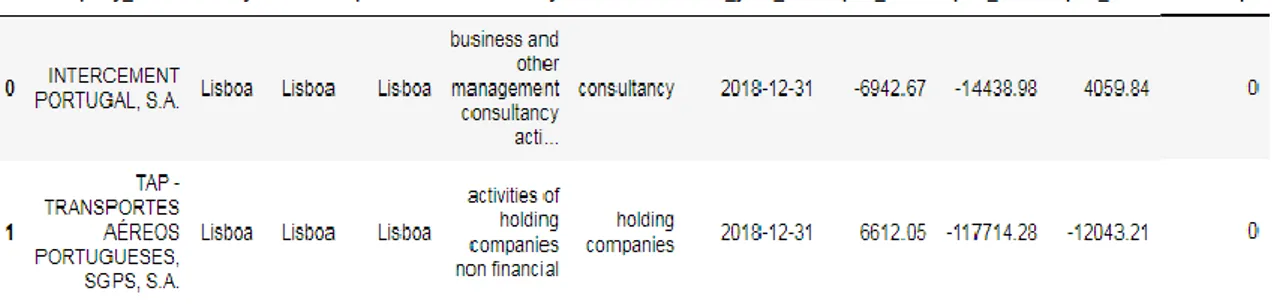
The final dataset contains a single company in each row and financial ratios for each year as well as the target variable “bankrupt” as columns.
Figure 1: Extract from the dataset
Within the bankrupt company data there were eight data entries not covering an entire financial year. For those companies the financial figures were extrapolated according to the 30/360 day-count convention (Brealey et al, 2011). This adjustment was necessary in order to make those companies comparable to the other companies where a full financial year was provided. The financial ratios used are from the following categories: liquidity ratios, leverage ratios and profitability ratios (Barboza et al, 2017). In addition to the ratios the variables consist out of different figures such as sales, total assets and number of employees (see Table A1).
The data exported from “sabi” contains missing values and zero values. The zero values could either result from reported zero values or due to a lack of information. For the purpose of the following analysis it was assumed that those zero values are due to reported zeros (Kapil et al, 2019). In order to keep the high number of data entries within the dataset, the missing values were imputed. Therefore, two different strategies were used. Firstly, the missing values were imputed with the median value of each corresponding variable. Secondly, the missing values were imputed with the mean value of each corresponding variable (Géron, 2017). Since the first strategy delivered slightly better results for the Random Forest model and delivered with
7
negligibly different results for the Logistic Regression this strategy was used for the final prediction.
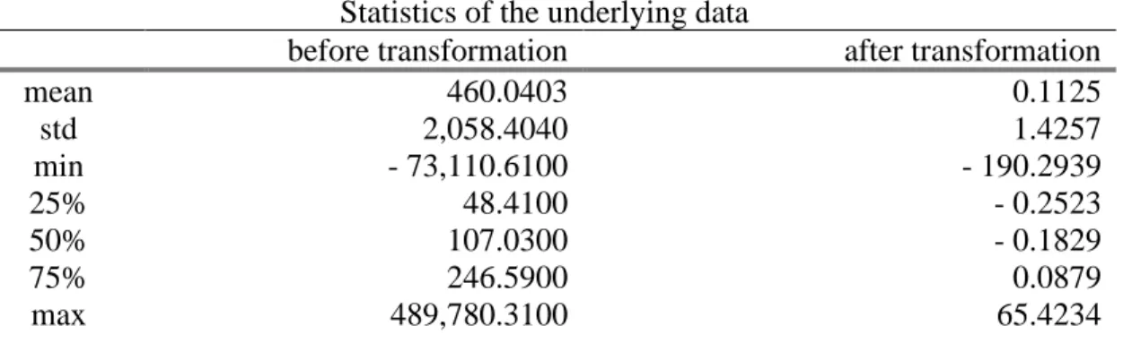
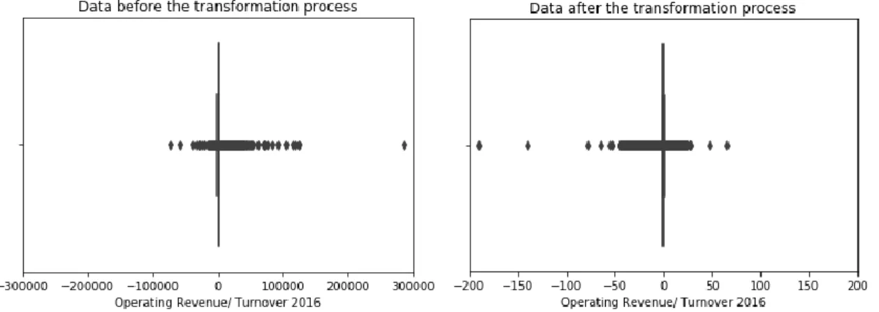
In addition, the data is skewed. This might be the result of the large dataset containing companies with different sizes and from various industries, which could lead to different characteristics within the financial statement data (Baetge, 2002). Skewed data means that the mean is typically lower or higher than the median of the underlying data (Brooks, 2014). This data needs to be adjusted, as the Logistic Regression is sensitive to skewed data. Since the dataset contains from low to high and positive plus negative values, the “Yeo-Johnson” transformation was used. This transformation package reduces skewness of the data and approximates normality (Yeo et al, 2000).
It was checked whether the companies within the dataset are unique data entries. In 709 cases the same company name appeared at least twice within the dataset. For those cases it was checked whether their data entries display the same company. As these companies do not share the same purpose and show different financial ratios, it is assumed that they are unique companies. Therefore, those companies were kept within the dataset.
Within the dataset multicollinearity occurs, meaning that some independent variables are highly correlated with other independent variables (Brooks, 2014). Variables with perfect multicollinearity were adjusted and not kept within the model, as they share the exact same relationship (Brooks, 2014). Variables showing near multicollinearity as a result of the financial ratio calculation were kept within the model, as this correlation will always occur and will hold over the sample of collected data (Brooks, 2014), (Jabeur, 2017).
The independent variables within the dataset such as number of employees, profit margin and net income are measured in different units. For the performance of the Logistic Regression model the data had to be normalized. Since the extreme values within the dataset are important
8
as stated before and the effect of those values needs to be kept within the model, the z-score was used to normalize the data. The z-score formula is the following:
𝑧 = 𝑥− 𝜇𝜎 , (1)
where 𝑧 is the normalized value, 𝑥 is the original value, 𝜇 is the mean of the variable and 𝜎 is standard deviation of the variable (see Table A2 and Figure A1) (Kelleher et al, 2015), (Géron, 2017).
In order to overcome the heavy imbalance of the dataset, the Synthetic Minority Over-sampling Technique (SMOTE) was used to adjust the class distribution (Chawla et al, 2002). This technique is based on an algorithm which generates new samples of the underrepresented class, in this case bankrupt companies. For the interpolation of the minority class, the algorithm is considering a sample 𝑥𝑖 of this class, taking one of the k nearest-neighbors 𝑥𝑧𝑖 and is creating
a new sample as follows:
𝑥𝑛𝑒𝑤 = 𝑥𝑖 + 𝜆 × (𝑥𝑧𝑖 − 𝑥𝑖), (2)
where 𝜆 is a random number within the range of 0 and 1 (Lemaitre et al, 2016). In order to keep a high number of data entries within the dataset an over-sampling technique is used instead of an under-sampling technique (Kelleher et al, 2015). By means of SMOTE the model is trained on an artificially balanced dataset, in this case 262,128 data entries for both classes. Hence the bankrupt company class contains a very high number of artificially imputed data entries. Outliers within the data are values far away from the mean, either invalid outliers which are the result of errors or valid outliers which are correct values. In the underlying data valid outliers occur. Those extreme values such as high negative or high positive values might be important for the bankruptcy prediction model. Those values might display a very good or bad health status of a company. Therefore, they were kept within the dataset (Kelleher et al, 2015).
9 4. Research methodology
As mentioned before, initially selected variables where ratios extracted from the “sabi” provider.
The data was randomly split into train and test data. The training data was used for building and fitting the models whereas the test data was used for testing the models and calculating the predictive power of the models (Geng et al, 2015). 80% of the data is used for training the models and 20% is used for testing the models. Within the train data there are 262,128 healthy companies and 723 bankrupt companies and within the test data there are 65,532 active companies and 177 bankrupt companies. (Geng et al, 2015) In order to train the model on a balanced dataset the bankrupt companies within the training data were extrapolated as described in the previous chapter.
The Logistic Regression can be used as a binary classifier and in the purpose of this paper estimating the probability of a company belonging to a certain class, either the class bankrupt companies or the class non-bankrupt companies. If the probability is by default greater than 50%, the model predicts that the company belongs to the bankrupt company’s class otherwise the model predicts that the company does not belong to the bankrupt company’s class but instead it belongs to the healthy company’s class (Géron, 2017).
The Logistic Regression approach uses the sigmoid function in order to transform the regression model so that the predicted values are bound within 0 and 1. The logistic function would be
𝐹(𝑧𝑖) =1 + 𝑒𝑒𝑧𝑖𝑧𝑖= 1 + 𝑒−𝑧𝑖1 , (3)
where z is a random variable and e the exponential under the logit approach (Brooks, 2014). The estimated Logistic Regression model would be
𝑃𝑖 = 1
10 where 𝑃𝑖 is the probability that 𝛾𝑖 = 1 (Brooks, 2014).
The Random Forest model is an ensemble of multiple decision trees (Barboza et al, 2017), (Géron, 2017). When growing each Decision Tree, the Random Forest algorithm searches for the best feature among a random subset of features when splitting the node. This results in a greater diversity of trees which leads to a better model performance. This classifier is used to predict whether a company belongs to the bankrupt or healthy company class. In addition, the Random Forest model calculates for each variable a score which indicates how much this specific variable contributes to the classification decision. This is known as feature importance (Géron, 2017).
Both models were implemented utilizing libraries in the programming language Python, namely Scikit-Learn.
In order to find the best classifier of each model, Grid Search was used. Grid Search seeks for the best parameters of an algorithm (hyperparameters) within a given search space of hyperparameters using cross validation (Géron, 2017). Grid Search was mainly used to find the best estimator for the Random Forest model. In order to apply a consistent research approach, it was also used to optimize the hyperparameters for the Logistic Regression model.
With the aim of enhancing the robustness of the results and mitigating the issue of overfitting, five times repeated random sub-sampling validation was applied (Geng et al, 2015).
From a stakeholder’s perspective the costs of a model classifying an unhealthy company as healthy (Type I Error) are higher than the costs of a model classifying a healthy firm as unhealthy (Type II Error). A misclassification of Type I Error is a loss of an investment or debt that will not be reimbursed in case of bankruptcy (du Jardin, 2010). In contrast a Type II Error results in opportunity costs for instance missed gains from an investment. It could also result in higher costs or difficulties for the misclassified company. Higher costs in the sense of higher
11
interest rates for loans, restricted terms from suppliers or difficulties in raising capital. Whether the one or the other error is more critical depends on the view of the user (Gepp et al, 2015). For the purpose of this work, the goal is to minimize the Type I Error, since it results in higher costs (du Jardin, 2010).
As performance measures, different tools were used. First, a confusion matrix was examined in order to check for the model’s robustness. The confusion matrix gives an overview on how many companies were correctly classified as healthy or bankrupt companies and how many companies were falsely classified as healthy or bankrupt companies (Barboza et al, 2017). Since the purpose of the paper is to decrease the Type I Error, the sensitivity or true positive rate (TPR) needs to be maximized. Sensitivity is calculated as follows:
𝑠𝑒𝑛𝑠𝑖𝑡𝑖𝑣𝑖𝑡𝑦 = (𝑇𝑃+𝐹𝑁)𝑇𝑃 , (5)
where TP is True Positive, and FN is False Negative. True Positive means that bankrupt firms were correctly classified as bankrupt, in contrast False Negatives are the bankrupt companies falsely classified as healthy (Géron, 2017).
Nonetheless it is important not to ignore the specificity or true negative rate (TNR) which is calculated as follows:
𝑠𝑝𝑒𝑐𝑖𝑓𝑖𝑐𝑖𝑡𝑦 = (𝑇𝑁+𝐹𝑃)𝑇𝑁 , (6)
where TN is True Negative, and FP is False Positive. True Negatives are the non-bankrupt companies correctly classified as healthy companies and the False Positives are the healthy companies falsely classified as bankrupt companies (Géron, 2017).
12
As stated before, there is a preference for maximizing sensitivity since this is translated into losses for creditors whereas specificity is the threshold for gain of the evaluated company (Barboza et al, 2017).
Second, the Receiver Operating Characteristic Curve (ROC) Curve was applied and the Area Under ROC Curve (AUC) was calculated. The ROC Curve plots the true positive rate against the false positive rate (Géron, 2017). In order to accept the model, the ROC AUC score had to be higher than 0.5, since 0.5 displays a random guess. The closer the ROC AUC score is to 1, the more accurate the prediction and the higher the predictive power (Barboza et al, 2017).
5. Results and discussion
Overall it can be stated, that both classifiers achieved good prediction results compared to a random guess classifier.
Results Decision threshold 0.1 0.3 0.5 0.8 Random Forest Classifier Sensitivity 0.99 0.90 0.68 0.30 Specificity 0.23 0.60 0.85 0.98 Logistic Regression Classifier Sensitivity 0.99 0.89 0.71 0.34 Specificity 0.09 0.34 0.79 0.97 Table 1: Results
Best results were achieved with the following strategies. For the Random Forest model, the missing values were imputed with the median value of each corresponding variable, and by means of SMOTE the training data was balanced artificially. For the Logistic Regression model, the same previous steps were executed as for the Random Forest model, in addition the data was normalized, and the skewed data was adjusted as described before.
13
The confusion matrix was conducted for different decision threshold in order to deal with the trade-off between sensitivity and specificity (see Figure A2 and Figure A3) (Géron, 2017). Even though the goal of this paper was to maximize the correctly classified bankrupt companies which means maximizing the sensitivity, it is still important to deal with the trade-off between the correctly classified bankrupt companies and the correctly classified healthy companies. A model classifying all companies as bankrupt would result in a very high sensitivity but would also be a moronic classifier, therefore good enough results had to be achieved for the specificity (du Jardin, 2010), (Barboza et al, 2017). Both classifiers have a better sensitivity-specificity trade-off if the decision threshold is a lower than the default decision threshold of 0.5. The default decision threshold means that if the classifier is predicting a probability of a company being bankrupt higher than 0.5, the classifier predicts this company as a bankrupt company. For a probability lower than 0.5, the classifier predicts that the company is healthy (Géron, 2017). This threshold was set to 0.1, 0.3, 0.5 and 0.8 for the Logistic Regression model and the Random Forest model. The lower the threshold the higher the sensitivity and the lower the specificity and vice versa (see Table 1). In addition, it can be said that a decision threshold lower than the default delivers better prediction results for both classes. Not only the correct classification of the bankrupt companies could be maximized but also the incorrect classification of the healthy companies could be minimized while considering the trade-off between sensitivity and specificity as well as the goal of maximizing the number of correctly classified bankrupt companies.
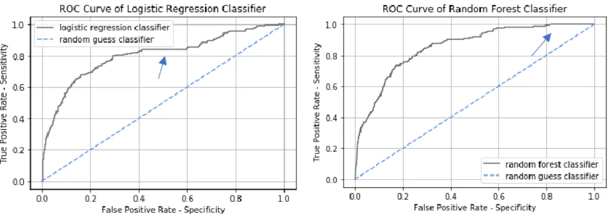
Plotting the ROC Curve delivers the following.
14
Figure 2: ROC Curve of Logistic Regression and Random Forest classifier (Géron, 2017)
The ROC Curve of each model stays away from the dotted line representing a random guess classifier, which means that the classifier performs good. Nevertheless there is still space for improvement, since the curve does not fill the space in the upper-left corner (Géron, 2017). The straight line within the curve might be a result of the duplicates due to the strategy of imputing the missing values within the dataset.
Since the training ROC AUC score of 0.92 for the Random Forest model and 0.82 for the Logistic Regression are higher than the testing ROC AUC score of 0.77 for the Random Forest model and 0.75 for the Logistic Regression, the model might overfit. This indicates that the model performs well on training data but not as good on test data (Alaka et al, 2018). In order to prevent heavy overfitting, more restrictions were used to find the best estimator. For the Random Forest model, the hyperparameters such as maximum depth and maximum features and for the Logistic Regression model the hyperparameter maximum iterations were decreased. This prevents that the model is learning every exception within the training data and is performing very well on this data but unfortunately bad on the test data (Géron, 2017).
For the Logistic Regression it can be said that increasing variables with a positive coefficient results in an increasing likelihood of filing for bankruptcy in 2017. Whereas increasing variables with a negative coefficient results in a decreasing likelihood of filing for bankruptcy in 2017 (see Table A3) (López Iturriaga et al, 2015), (Alaka et al, 2018).
15
For the Random Forest model, it can be stated that variables with a higher score of importance contribute more to the classification decision. It cannot be disclosed whether a high score leads to a positive or negative impact on the probability of filing for bankruptcy in 2017 (Yeh et al, 2012), (López Iturriaga et al, 2015).
Overall, the Random Forest model achieves slightly better results than the Logistic Regression. The developed models described in the previous chapter are good predictors and can both be used as a basis for further studies. It can be recognized that the years closer to the event of bankruptcy tend to contribute more to the classification decision. Even though for both classifiers different sets of variables contributed to the classification decision (see Table A3 and
Table A4).
Although the results show a good prediction accuracy this study reveals some limitations. The quality of the data used in this study could be improved. Given the time frame of the creation of this paper the missing values were imputed with the median value of each corresponding variable. Additional research on the practices of imputing missing values could lead to a higher quality dataset and therefore might result in a higher prediction performance (Kelleher et al, 2015). In addition to the missing values, the dataset contains zero values, as mentioned before it was assumed that these zeros meant to be reported as zeros. There could also be additional analysis in further studies on whether these zeros are reported zeros or whether there are other assumptions and solutions which could lead to a higher quality within the dataset (Kapil et al, 2019).
Since the missing values were imputed with the median value of each variable, there are duplicates within the dataset. Eventually those duplicates represent companies from the healthy and unhealthy class and could therefore not lead to a better classification decision of the models (Kelleher et al, 2015).
16
Additionally, all variables used are accounting data and therefore internal company data. Various papers already discussed the drawback, since these variables are information from the past and therefore models using only accounting information are not the best fit for predicting the future (Baetge, 2002), (Yeh et al, 2012). Other paper used macroeconomic and market-based variables or non-financial indicators in addition to financial statement data. These variables and eventually the region within Portugal could also result in a better prediction power of the models used in this paper (Hernandez Tinoco et al, 2013), (Geng et al, 2015), (Barboza et al, 2017). Nevertheless, accounting data is crucial for bankruptcy prediction, as it reflects the health status of a company (Hernandez Tinoco et al, 2013).
The methods used could also be improved, since in other studies concerning bankruptcy prediction the Extreme Gradient Boosting algorithm outperformed the Logistic Regression and Random Forest model (Ziȩba et al, 2016). This method could also be used for the underlying data of this study to eventually improve the results of this research question. For simplicity purposes, this work was limited to two algorithms.
For the purpose of this work there was no selection in terms of industry or size of the companies within the dataset. The data was kept generally as it was collected. There is always a trade-off between an eventually more precise prediction method and reducing the data due to industry, size or other characteristics. Keeping the dataset as it is, with very different companies concerning characteristics could also be an advantage, since there is no bias and a higher generalization ability within the dataset (Geng et al, 2015).
The afore mentioned feature importance only lasts until a model is changed. If the model is adjusted, the feature importance might change as well. In addition, it is impossible to state in which direction the influence of those variables will affect the likelihood of bankruptcy (Lundberg et al, 2019).
17 6. Conclusion
Within this study financial statement data from various Portuguese companies for a time frame of five years prior to the event of bankruptcy in 2017 was used. The dataset included 327,642 healthy and 900 unhealthy companies and is therefore heavily imbalanced. Even though there are some limitations concerning the quality of the data and the methodology used, this study provides good results concerning the prediction of bankruptcy. Those results can be used as a basis for further studies concerning bankruptcy prediction in Portugal.
The two models, Logistic Regression and Random Forest, were able to classify the bankrupt companies with good results. Although the focus of this paper is to maximize the number of bankrupt companies being correctly classified as bankrupt, both models were able to classify also the healthy companies correctly with good results. Therefore, the default decision threshold was decreased, which resulted in a better trade-off between the two classes being correctly classified.
Future studies concerning Portuguese corporate bankruptcy should consider other relevant data besides financial statement data, such as market-based and macroeconomic data (Hernandez Tinoco et al, 2013). Additionally, further studies should use other machine learning models which might outperform the models used in this study and might improve the classification results (Ziȩba et al, 2016).
Even though there is space for improvement it can be stated that the results obtained from this study are good initial results for further studies in the field of corporate bankruptcy. As the decision threshold is lower than the default decision threshold the two models are able to classify the companies correctly meaning that the trade-off between sensitivity and specificity improved. Therefore, it can be stated that the Logistic Regression and Random Forest model are able to predict the corporate bankruptcy of the selected Portuguese companies.
XVIII References
Underlying Code. 2020. Sina Bruhn.
https://github.com/sinabru/corporate_bankruptcy_prediction
Alaka, H. A., Oyedele, L. O., Owolabi, H. A., Kumar, V., Ajayi, S. O., Akinade, O. O., and Bilal, M. 2018. "Systematic review of bankruptcy prediction models: Towards a framework for tool selection." Expert Systems with Applications, 94: 164–184.
Altman, E. I. 1968. "Finacial Ratios, Discriminant Analysis and the Prediction of Corporate Bankruptcy." The Journal of Finance, 23(4): 589–609.
Baetge, J. 2002. "Die Früherkennung von Unternehmenskrisen anhand von Abschlusskennzahlen." Der Betrieb, 44: 2281–2287.
Bankruptcy - Portugal. 2006. European Commision.
https://ec.europa.eu/civiljustice/bankruptcy/bankruptcy_por_en.htm (accessed October 25, 2019).
Barboza, F., Kimura, H., and Altman, E. 2017. "Machine learning models and bankruptcy prediction." Expert Systems with Applications, 83: 405–417.
Beaver, W. H. 1966. "Financial Ratios As Predictors of Failure." Journal of Accounting Research, 4: 71–111.
Bell, T. B., Ribar, G. S., and Verchio, J. 1990. "Neural Nets Versus Logistic Regression: A Comparison of Each Model’s Ability to Predict Commercial Bank Failures." Proceedings of the University of Kansas Symposium on Auditing Problems, 10: 28–53.
XIX
Brealey, R. A., Myers, S. C., and Allen, F. 2011. Principles of Corporate Finance. New York: McGraw-Hill/ Irwin.
Brooks, C. 2014. Introductory Econometrics for Finance. Cambridge: Cambridge University Press.
Chawla, N. V., Bowyer, K. W., Hall, L. O., and Kegelmeyer, W. P. 2002. "SMOTE: Synthetic Minority Over-sampling Technique." Journal of Artificial Intelligence Research, 16(1): 321–357.
Chua, L. K., and Dwyer, D. W. 2009. "Moody’s KMV RiskCalc v3.1 Portugal." Moody’s KMV: 1–27.
du Jardin, P. 2010. "Predicting bankruptcy using neural networks and other classification methods: The influence of variable selection techniques on model accuracy." Neurocomputing, 73(10–12): 2047–2060.
du Jardin, P. 2015. "Bankruptcy prediction using terminal failure processes." European Journal of Operational Research, 242(1): 286–303.
Geng, R., Bose, I., and Chen, X. 2015. "Prediction of financial distress: An empirical study of listed Chinese companies using data mining." European Journal of Operational Research, 241(1): 236–247.
Gepp, A., and Kumar, K. 2015. "Predicting Financial Distress: A Comparison of Survival Analysis and Decision Tree Techniques." Procedia Computer Science, 54: 396– 404.
XX Sebastopol: O’Reilly.
Gilbert, L. R., Menon, K., and Schwartz, K. B. 1990. "Predicting Bankruptcy for Firms in Financial Distress." Journal of Business Finance & Accounting, 17(1): 161–171.
Hernandez Tinoco, M., and Wilson, N. 2013. "Financial distress and bankruptcy prediction among listed companies using accounting, market and macroeconomic variables." International Review of Financial Analysis, 30: 394–419.
Jabeur, S. Ben. 2017. "Bankruptcy prediction using Partial Least Squares Logistic Regression." Journal of Retailing and Consumer Services, 36: 197–202.
Kapil, S., and Agarwal, S. 2019. "Assessing Bankruptcy of Indian Listed Firms Using Bankruptcy Models, Decision Tree and Neural Network." International Journal of Business and Economics, 4(1): 112–136.
Kelleher, J. D., Mac Namee, B., and D’Arcy, A. 2015. Fundamentals of Machine Learning for Predictive Data Analytics. Cambridge: MIT Press.
Krommes, W. 2011. Handbuch Jahresabschlussprüfung. Wiesbaden: Gabler.
López Iturriaga, F. J., & Sanz, I. P. 2015. "Bankruptcy visualization and prediction using neural networks: A study of U.S. commercial banks." Expert Systems with Applications, 42(6): 2857–2869.
Lundberg, S. M., Erion, G. G., and Lee, S.-I. 2019. "Consistent Individualized Feature Attribution for Tree Ensembles." University of Washington, March 2019. http://arxiv.org/abs/1802.03888.
XXI
Ohlson, J. A. 1980. "Financial Ratios and the Probabilistic Prediction of Bankruptcy." Journal of Accounting Research, 18(1): 109-130.
Over-sampling. 2016. Lemaitre, G., Nogueira, F., Oliveira, D., and Aridas, C. https://imbalanced-learn.readthedocs.io/en/stable/over_sampling.html#smote-adasyn (accessed December 29, 2019).
Pereira Leal, C., and Machado-Santos, C. 2007. "Insolvency Prediction in the Portuguese Textile Industry." European Journal of Finance and Banking Research, 1(1): 16–27.
sabi. 2019. Moody’s Analytics. https://sabi.bvdinfo.com/version-20191128/Login.serv?product=sabineo&SetLanguage=en&UIMode=Advanced
(accessed December 2, 2019).
Shin, K. S., Lee, T. S., and Kim, H. J. 2005. "An application of support vector machines in bankruptcy prediction model." Expert Systems with Applications, 28(1): 127–135.
Yeh, C.-C., Lin, F., and Hsu, C.-Y. 2012. "A hybrid KMV model, random forests and rough set theory approach for credit rating." Knowledge-Based Systems, 33: 166–172.
Yeo, I.-K., and Johnson, R. A. 2000. "A New Family of Power Transformations to Improve Normality or Symmetry." Biometrika, 87(4): 954–959.
Ziȩba, M., Tomczak, S. K., and Tomczak, J. M. 2016. "Ensemble boosted trees with synthetic features generation in application to bankruptcy prediction." Expert Systems with Applications, 58: 93–101.
XXII Appendices
Variable Description
oprev_turn_year Operating revenue/ Turnover in TEUR per Year netinc_year Net Income in TEUR per Year
totass_year Total Assets in TEUR per Year
sheq_year Shareholders' equity in TEUR per Year rosf_year Return on Shareholders' Funds in % per Year roce_year Return on Capital Employed in % per Year rota_year Return on Total Assets in % per Year
pm_year Profit Margin in % per Year
nato_year Net Assets Turnover in % per Year
ic_year Interest Cover in % per Year
sto_year Stock Turnover in % per Year
colpe_days_year Collection period in Days per Year crepe_days_year Credit Period in Days per Year
curr_year Current Ratio in % per Year
liqr_year Liquidity Ration in % per Year
shliqr_year Shareholders Liquidity Ratio in % per Year gearing_year Gearing in % per Year
prof/empl_year Profit per Employee in TEUR per Year
operrev/empl_year Operating Revenue per Employee in TEUR per Year costsofempl_operrev_year Costs of Employee/ Operating Revenue in % per Year avcostsofempl/year_year Average Cost of Employee in TEUR per Year
sharefunds/empl_year Shareholder Funds per Employee in TEUR per Year wc/empl_year Working Capital per Employee in TEUR per Year totassets/empl_year Total Assets per Employee in TEUR per Year numofempl_year Number of Employees per Year
sales_year Sales in TEUR per Year
wc_year Working Capital in % per Year
ebit_year EBIT in TEUR per Year
Table A1: Variables used as underlying data (Moody’s Analytics, 2019)
Statistics of the underlying data
before transformation after transformation
mean 460.0403 0.1125 std 2,058.4040 1.4257 min - 73,110.6100 - 190.2939 25% 48.4100 - 0.2523 50% 107.0300 - 0.1829 75% 246.5900 0.0879 max 489,780.3100 65.4234
XXIII Feature Coefficient totass_2015 0.471837 numofempl_2015 0.413567 sales_2012 0.263196 operv_turn_2014 0.219752 totass_2014 0.213423 liqr_2012 -0.429840 netinc_2015 -0.516671 sales_2016 -0.523971 oprev_turn_2016 -0.561352 ebit_2015 -0.563105
Table A3: Top 5 and bottom 5 coefficients of the Logistic Regression classifier
Feature Importance ic_2016 0.209813 prof/empl_2016 0.095802 numofempl_2014 0.076891 crepe_days_2016 0.067061 oprev_turn_2012 0.051403 numofempl_2016 0.048355 pm_2016 0.046546 netinc_2015 0.036750 sales_2016 0.028675 netinc_2016 0.024053
Table A4: Top 10 features by importance of the Random Forest classifier
Figure A1: Visualization of the data before and after the transformation process
XXIV
Figure A2: Confusion Matrices of the Logistic Regression classifier for different decision thresholds (Géron, 2017)
XXV
Figure A3: Confusion Matrices of the Random Forest classifier for different decision thresholds (Géron, 2017)