ISBN: 978-9952-8071-4-1
EMERGING ISSUES
IN THE NATURAL AND
APPLIED SCIENCES
Academic book
“PROGRESS”
LCC: AY10-29 UDC: 002
Editor-in-chief: J.Jafarov Technical editor A. Xankishiyev
Editorial board:
Ángel F. Tenorio, Prof. Dr.
Polytechnic School, Pablo de Olavide University (Spain)
Maybelle Saad Gaballah, Prof. Dr.
National Research Centre, Cairo (Egypt)
Manuel Alberto M. Ferreira, Prof. Dr.
ISCTE-Lisbon University Institute (Portugal)
Eugen Axinte, Prof. Dr.
"Gheorghe Asachi" Technical University of Iasi (Romania)
Sarwoko Mangkoedihardjo, Prof. Dr.
Sepuluh Nopember Institute of Technology (Indonesia)
Cemil Tunc, Prof. Dr.
Yuzuncu Yil University (Turkey)
Peng Zhou, Prof. Dr.
School of Medicine, Wake Forest University (USA)
Emerging issues in the natural and applied sciences. “Progress” LLC, Baku, 2012, 168 p.
This research book can be used for teaching modern science, including for teaching undergraduates in their final undergraduate course in all fields of natural and applied sciences. More generally, this book should serve as a useful reference for academics, sciences researchers.
ISBN: 978-9952-8071-4-1
© Progress IPS LLC, 2012 © IJAR, 2012
TABLE OF CONTENTS
Chapter 1.
Manuel Alberto M. Ferreıra, Marina Andrade
NUMERICAL METHODS TO COMPUTE SOJOURN TIMES IN JACKSON
NETWORKS DISTRIBUTION FUNCTIONS AND MOMENTS………..5 Chapter 2.
Abu Hassan Abu Bakar, Muhammad Asim Tufail, Wiwied Virgiyanti
KNOWLEDGE MANAGEMENT INFRASTRUCTURE CAPABILITIES
AS PREDICTORS OF PROJECT BENEFITS...28 Chapter 3.
José Antónıo Fılıpe, Manuel Alberto M. Ferreira, Manuel Coelho, Maria Isabel C. Pedro
FISHERIES PROBLEMS AND BUREAUCRACY IN AQUACULTURE.
AN ANTI-COMMONS VIEW...51 Chapter 4.
Ganjar Samudro,Sarwoko Mangkoedihardjo
EVAPOTRANSPIRATION UNITS FOR SANITATION INFRASTRUCTURE………....65 Chapter 5.
Abu Hassan Abu Bakar, Wiwied Virgiyanti, Muhammad Asim Tufail
KNOWLEDGE MANAGEMENT PROCESSES AND COMPETITIVE
ADVANTAGE IN CONSTRUCTION INDUSTRY...81 Chapter 6.
Marına Andrade, Manuel Alberto M. Ferreıra
THE PROBLEM OF CIVIL AND CRIMINAL IDENTIFICATION - BAYESIAN
NETWORKS APPROACH………...103 Chapter 7.
Ahmed Mohammed Kamaruddeen, Nor'Aini Yusof, Ilias Said
DIMENSIONS OF FIRM INNOVATIVENESS IN HOUSING INDUSTRY...118 Chapter 8.
Syed M. Nurulain
ACUTE ORGANOPHOSPHORUS POISONING-APPROACHES
FOR TREATMENT...114 Chapter 9.
I.C. Madufor, U.E. Itodoh, M.U. Obidiegwu, M.S. Nwakaudu, B.C. Aharanwa
INHIBITION OF ALUMINIUM CORROSION IN ACIDIC MEDIUM BY
M.A.M. Ferreıra, M. Andrade. Numerical methods to compute sojourn times in Jackson networks distribution functions and moments.
Emerging Issues in the Natural and Applied Sciences 2012; 2(1), 5-27.
DOI: 10.7813/einas.2012/2-1/1
NUMERICAL METHODS TO COMPUTE SOJOURN
TIMES IN JACKSON NETWORKS DISTRIBUTION
FUNCTIONS AND MOMENTS
1,2Prof. Dr. Manuel Alberto M. Ferreıra, Dr. Marina Andrade University Institute of Lisbon, BRU/UNIDE, Lisboa (PORTUGAL)
E-mails: [email protected], [email protected] DOI: 10.7813/einas.2012/2-1/1
ABSTRACT
Jackson queuing networks have a lot of practical applications, mainly in human and technologic devices. For the first case, an example are the healthcare networks and, for the second, the com-putation and telecommunications networks. Evidently the time that one customer - a person, a job, a message … – spends in this kind of systems, its sojourn time, is an important measure of its perfor-mance, among others. In this work the practical known results about the sojourn time distribution are collected and presented. And an emphasis is put on the numerical methods applicable to compute the distribution function and the moments.
Keywords: Jackson networks, sojourn time, network flow
equ-ations, randomisation procedure. 1
This work was financially supported by FCT through the Strategic Project PEst-OE/EGE/UI0315/2011.
2
The paper “Sojourn Times in Jackson Networks” related with this one was presented in the Conference Aplimat 2012 as a Plenary Lecture and selected to Aplimat-Journal of Applied Mathematics.
1. INTRODUCTION
In this work it is intended to present some problems and re-sults that arise in the study of the sojourn time in Jackson networks of queues. These networks have many applications, namely in the modelling of healthcare, computation and telecommunications net-works. And a customer sojourn time, in this kind of system, is evi-dently an important element to be considered in its performance evaluation. Maybe the most important.
The model of network to be considered in this paper is briefly described in section 2. The main objective of section 3 is the presen-tation of formula (10) that, in some situations allows the sojourn times moments exact computation. In section 4 it is given a nume-rical method for the sojourn times distribution function and any order moments computation, adequate to any Jackson network.
2. GENERAL RESULTS AND EXAMPLES
Along this work, the sojourn times in a class of Markovian net-works of queues, introduced initially by Jackson, see (1-2), will be studied. They are called Jackson networks and have only one class of customers. They are composed of
J
nodes numbered1,2,..., J. It is usual to putU
1
,
2
,...,
J
.In each node there is only one server, a queue discipline “first-come-first-served” (FCFS) and an infinite waiting capacity.
They are open networks since any customer may enter or abandon it.
The exogenous arrivals-that is: from the outside of the net-work- process at node
j
is a Poisson Process at rate
j,
j
U
, in-dependent of the exogenous arrivals processes to the other nodes. It is stated that
J j j 1 .
The service times at node
j
are independent and identically distributed, having exponential distribution with parameter
j,
j
U
, and independent from the other nodes service times.After the completion of a service at node
j
, a customer is immediately directed to nodel
with probabilityp
jl, or abandons thenetwork with probability
J l jl jp
j
U
q
1,
1
.These probabilities are not influenced by the movements of the other customers in the network. The
p
jl matrix is called P . The matrix P is called the commutation matrix and thep
jl commutation probabilities.The total arrivals rate, exogenous and endogenous-that is: from the other nodes of the network- at node
j
,
j satisfies the net-work traffic equations:J
j
p
J l lj l j j,
1
,
2
,...,
1
(1).The state of the network at instant t is given by
t
N
t
N
t
N
1,...,
J , whereN
j
t
is the number of customers atnode
j
in instantt, j 1,2,...,J. N is the population process.If the traffic intensity
j
J
j j j
1
,
1
,
2
,...,
the process
N
t
N
has stationary, or equilibrium, distribution, see for instance (3),
n n n
n j J J j j n j j J j ,..., 2 , 1 , 0 , 1 ,..., , 1 2 1
(2).The distribution (2) is a product form distribution, see for instance (4-5).
Calling
S ,
jW
j andX
j the sojourn, waiting and service, res-pectively, times of a customer at nodej
j j j
W
X
S
(3).The Jackson networks sojourn times considered in this paper are those of typical customers that, arriving at the network, find the population process in an equilibrium state. Call
S
the sojourn time in the network, that is: the time that goes between the arrival at the network and the departure of one of those customers from it. If in its path it traverses the nodes1,2,...,l,
S
S
1
S
2
...
S
l.To study the sojourn time, the following is important:
- A network has “feedback” if a customer may come back to the same node after the completion of its service, immediately or in a future instant,
- A network without “feedback” is an “acyclic” one,
- A network has “overtaking” if a customer can “overtake” another one taking an alternative path between two nodes. Then three examples of typical Jackson networks usually con-sidered in the study of sojourn times are presented. It may be said that more complex Jackson networks are integrated by networks ful-filling the properties of these examples, in a modular way.
Simple Queues Series
For this Jackson network
otherwise
0
1
,...,
2
,
1
,
1
if
,
1
l
j
j
J
p
jlJ
j
J
j
j0
,
2
,..,
and
,
1
,
2
,...,
,
j 1
. Fig. 1 isFig. 1. Simple Queues Series
Some important results are:
- All customers’ flows, in this network, at stationary state, are Poisson Processes. It is a consequence of it, in stationary state, that the departure process from an M/M/1 queue is a Poisson Process, see for instance (6),
- The sojourn times in the various nodes are independent random variables. In (6) it is presented a demonstration of this statement based on the reversibility concept,
- The sojourn time at node
j
is an exponential random variable with parameter
j
,
j
1
,
2
,...,
J
,- The waiting times are dependent random variables. See also (6).
So the sojourn time study in these networks has no difficulty. The same is not true for the waiting time.
M/M/1 Queue with Instantaneous Bernoulli Feedback
It is a network with a single node.
J
1
,p
11p
,
q
1 1
p
andp
1
, where
1 and
1, see Fig. 2.Call
S
m the thm customer sojourn time in the network. So, if it is served
k
times
i
mk d mk i mk mk i m m a m m m t t t t t t t t S 0 1 1 2 0 2 1 0 1 ... (4) where-
t
ml0
t
iml is the time that the customer spends passing by the service system in the thl time, given by the difference between the th
l output (0) instant from the server and the one of the th
l junction (i-input) to the queue,
-
t
m01
t
ma1 is the time that the customer spends passing by the service system for the first time, given by the difference between the first output (0) instant from the server and the one of the arrival (a) to the queue,- mki
d mk
t
t
is the time that the customer spends passing by the service system for the last time, given by the difference between the departure (d) instant from the network and the one of the kthjunction (i) to the queue.
Note that K , the number of times that the customer passes by the server, is a random variable andP
K k
(1p)pk1,
k
1
,
2
,...
.
t
ml0
t
mli:
l
2
,
3
,...
is not a sequence of independent ran-dom variables, see (3).So it is not possible to make use of the usual statement to sum independent random variables. But it is possible to get an expres-sion to
P
S
m
t
that requires thek
steps transition probabilitiesfor the delayed Markovian renewal process
N t 0,t tli ,l01,2,...
o l
i conditioning to the number of times that
the customer returns to the queue.
Calling that transition probabilities matrix
Q
k
t
S
t
Q
t
p
p
V
P
k k i m
1
1
(5) where
is the iN (embedded version of
N
in the input ins-tants) stationary distribution,k
is the number of times the customer passes by the server andV
is a vector which entries are all 1.So, now, the situation is much more complicated than in the former case owing to the feedback.
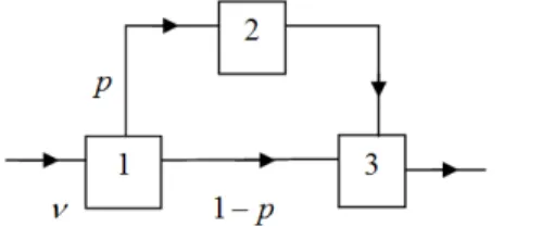
The Jackson Three Node Acyclic Network
It is a network with three nodes, Fig. 3, where
p
12p
,p
p
13 1
,p
23
1
,p
jl
0
in the other cases,
1
,3 , 2 , 0 j j
,
1
,
2
p
and
3
.In equilibrium, all customers’ flows are Poisson Process in this network.
Fig. 3. Jackson Three Node Acyclic Network
Consequently,
- The sojourn time at node
j
is a random variable exponen-tially distributed with parameter
j
j,
j
1
,
2
,
3
.S
1 andS
2 are independent random variables as well asS
2 andS
3. This result is valid for any Jackson acyclic network:- Suppose that a customer follows a path
r
in a Jackson acyclic network with only one server at each node. If nodej
belongs to path
r
,S
j is such that
0
,
1
t
the
followed
path
is
r
e
t
S
P
j j j t(6)
and, if node
j
is the next to the customer after nodel
,S
j andl
S
are independent random variables. But,-
S
1 andS
3 are dependent random variables: (7) showed that, in fact,S
1 andS
3 are positively correlated. In (8) It is stated that if
1 (7) 1 1 1 1 1 2 2 1 2 3 2 1 3 1 3 2 1 3 2 1 and if p 2 1 2 3 2 1 3 1 3 2 1 2 3 2 1 3 2 1 2 1 2 3 2 1 3 1 3 2 1 2 3 2 1 3 2 1 2 1 1 4 1 1 4 1 2 1 2 1 1 1 1 4 1 1 4 1 2 1 2 1 2 1 2 3 2 1 3 1 3 2 1 2 3 2 1 3 2 1 2 1 2 3 2 1 3 1 3 2 1 2 3 2 1 3 2 1 2 1 1 4 1 1 4 1 2 1 2 1 1 1 1 4 1 1 4 1 2 1 2 1 (8)verify both simultaneously it is possible to guarantee that
S
1 andS
3 are positively correlated in equilibrium.Why this happen? One explanation may be the following: - There are two alternative paths for a customer to go from
node 1 to node 3. And a customer that follows by node 2 may be overtaken by another one that goes directly from node 1 to node 3. So, a customer, when arriving at node 3, may meet there another one that was behind it at node 1 or even that had not arrived when it was there.
- These overtaking customers can delay a certain customer, when it arrives at node 3, for a longer time than that if they were not present. The number of these customers depends, partly, on the number of the customers that arrive while the customer that is being followed is in node 1, partly owing to the supposition of a FCFS discipline.
- Consequently, the time that a customer waits at node 3 de-pends on how much time it has waited at node 1.
Now the complication is due to the overtaking.
3. NETWORK FLOW EQUATIONS
The objective of this section is to present the so called “net-work flow equations” for the Jackson net“net-works, that allow the deduc-tion of formulae to the computadeduc-tion of sojourn times moments of any order, efficient in some situations.
Following the work of (9) call an arrival instant, endogenous or exogenous, at node j and + the departure instant from the network of the customer that arrived in , = 1, 2, … , , so
- is the remaining sojourn time, in the network, for the arrival at node j in the instant , = 1, 2, … , .
Call ℎ the Laplace Transform of the , = 1, 2, … , distribu-tion. As N is a strong Markov Process, and the network state pro-cess “seen by the arrivals” is in equilibrium, the , = 1, 2, … , and its Laplace Transforms are uniquely determined.
Dealing with the sojourn time as the life time of a Markov Pro-cess it is possible to show that the Laplace Transforms ℎ , = 1, 2, … , satisfy an equations system called the “network flow equa-tions”. That is, see (9),
- Being the probability distribution with Laplace Transform ℎ , there is a distribution probability with Laplace Transform
such as
ℎ ( ) + ( )= ( ) + ∑ ℎ ( ), ≥ 0 and = 1, 2, … , (9).
In Jackson networks without “overtaking” the Transforms ℎ and are identical for each j.
Given ℎ , = 1, 2, … , the Transforms , = 1, 2, … , are uni-quely determined by (9). The converse is also true since I – P, being
I the identity matrix, is invertible.
After (9), by successive derivations, - Network Flow Equations
For = 1, 2, … , and = 1, 2, …
= ! − + [ ]
+ !
! ( − )! ( ) + (10).
= ( − ) − (11). For r = 2 (10) assumes the form
= 2 − + [ ] + 2 ( ) + 1 , = 1, 2, … , (12).
Equality (12) defines a system of J equations and + unknowns. In general, when ≥ 2, the product terms involving the variables and ( ) prevent the exact computation of the sojourn times r order moments; there are too many unknowns and too few equations. In these cases other independent equations are needed to complement (12) in order to be possible to obtain exact solutions. When any pair of nodes in the network is connected by, in the maximum, one oriented path and = 0, = 1, 2, … , , and ( ) are independent for ≠ . The computation of + 1 is irrelevant since = 0, = 1, 2, … , . In this case (10) becomes a compact recursive formula that allows the computation of any order moments of the sojourn times, , = 1, 2, … , . For instance, as, in these conditions,
( ) =
− , = 1, 2, … , (13),
(12) assumes the form
= 2 − + [ ] + 2 − [ ], = 1, 2, … , (14).
Applying (14) to the simple queues series
= 2 − + [ ] + 2 − [ ], = 1, 2, … , − 1
= 2 −
that together with (11) gives
= ( − ) (16).
If those conditions are not fulfilled, in (9) it is suggested to identify adequate Martingale families in N as a process to determine independent equations to complement (10). Applying this proce-eding to the M/M/1 queue with instantaneous Bernoulli feedback it was obtained [ ] = 1 (1 − ) − (1 − ) + (1 − ) − (17) and [ ( ), ] = (1 − ) (1 − ) − (18).
4. SOJOURN TIMES DISTRIBUTIONS AND MOMENTS NUMERICAL COMPUTATIONS
Now it is given a general method, which key is the proceeding called “randomisation procedure”, to approximate “first passage times” distributions in direct time Markov Processes, being the sojourn times in queue systems a particular case.
Call ℵ = { ( ): ≥ 0} a regular Markov Process, in continuous time with a countable states space E and a bounded matrix infini-tesimal generator Q.
The elements of Q are designated by ( , ), , ∈ and ( ) = ∑ ∈ { } ( , ). ( ) designates the ( ) state pro-bability vector:
( ) = { ( ) = }, ∈ (19).
X models the evolution of a queue system during the sojourn
The states of E have two main components: i) The queue system state and ii) The “marked” customer position.
Be
- A the states subset that describes the system till the departure of the “marked” customer, and
- B the states subset that describes the system after the de-parture of that customer.
Evidently
- { , } is a partition of E,
- If T is the time that the process ℵ spends in A till attaining B, for the first time, T is precisely the sojourn time of the “marked” customer in the network.
It is supposed that ℵ will remain in B, with probability 1 after having attained it for the first time. In fact, as the evolution of the system after the departure of the “marked” customer is irrelevant, it may be supposed that B is a closed set. That is, the process ℵ can-not come back to A after reaching B. The quantity of interest is the T distribution function, ( ). Note that
( ) = { ≤ } = { ( ) ∈ } = 1 − { ( ) ∈ }, ≥ 0 (20)
since the presented hypotheses guarantee that { ≤ } = { ( ) ∈ }.
After (20) it is concluded that
- The problem of computing ( ) is equivalent to the one of the computation of the transient distribution of ( ) in A.
So it is necessary to compute the vector , ≥ 0. Being , ≥ 0, the ℵ n transition matrix,
= , ≥ 0 (21) and = ( ) = ! ∞ , ≥ 0 (22).
The “randomisation procedure” consists in using in (22) an equivalent representation; see (10):
= (− ) +1 = (− )
! (23)
∞
where
= + (24)
is called the “randomised matrix”. I is the identity matrix, and is a positive upper bound for the whole ( ), ∈ .
Note that, see (11-12),
- Although the equation (23) seems more complex than (22), it fulfils in fact more favourable computational properties. The most important is that R is a stochastic matrix while Q is not. Consequently, the computation using (23) is stable and using (22) is not,
- The “randomisation procedure” has an interesting probabilistic meaning, useful to determine bounds for ( ). In fact, being R a stochastic matrix, it defines a discrete time Markov Process
ℑ = { : = 0, 1, … } (25)
if it is assumed = (0). With this procedure, the relation between the processes ℵ and ℑ is quite simple as it will be seen next.
Extend the discrete time process ℑ to a continuous time Markov Process such that
i) The time intervals between jumps are exponential random
variables i.i.d. with mean 1⁄
ii) The jumps are commanded by R.
In (11) it is shown that the resulting process is precisely the original process ℵ; but when there is a sequence of jumps in ℑ from the state ∈ to itself, this will be noticed in ℵ as a long sojourn in state x.
So, the “randomisation procedure” may be interpreted as a sowing in the process ℵ with “fake” random jumps between the true jumps. The resulting process, designated by ℵ, at which the “fake” jumps are visible, has the same probabilistic structure than ℵ but with an advantage:
- The sequence of the jump instants inℵ, “fake” and “true”, is now a Poisson Process. This is not, in general, the case of ℵ. Note that is the state of ℵ in the instant of the nth jump, “fake” or “true”.
Suppose that ℵ reaches the set B in its nth
jump. Consequently the ℵ sojourn time, and so also the ℵ, in A is the sum of n exponen-tial independent random variables with mean 1⁄ . That is, the sojourn time has a n order Erlang distribution with parameter . Its distribution function will be designated , ( ).
Be ℎ( ) the probability that ℵ reaches B in its nth jump. Call the state probability vector of :
= (26). The quantities ℎ( ) are given by the equivalent formulae:
ℎ( ) = ⎩ ⎪ ⎨ ⎪ ⎧ ( ), = 0 ∈ ( ) ( , ), > 0 (27) ∈ ∈ or ℎ( ) = ⎩ ⎪ ⎨ ⎪ ⎧1 − ( ), = 0 ∈ ( ) − ( ), > 0 (28). ∈ ∈
Given the probabilities ℎ( ) and, noting that ∑∞ ℎ( )= 1, it is obtained
( ) = ℎ( ) , ( ), ≥ 0 (29),
∞
[ ] = 1 ( + 1) … ( + − 1)ℎ( ), = 1, 2, … (30).
∞
The formula (30) for m = 1 is
[ ] =1 [ ] (31)
being H the number of ℵ jumps till reaching B. Expression (31) is the Little’s Formula in this queues context.
Equation (29) allows obtaining simple bounds for ( ) that may, in principle, to become arbitrarily close. Equation (30) allows obtaining a lower bound for [ ], in principle, so close of [ ] as wished. So, given any integer ≥ 0
( ) ≤ ( ) ≤ ( ) (32)
( ) = ℎ( ) , ( ), ≥ 0 (33), ( ) = 1 − ℎ( ) , ( ), ≥ 0 (34) and [ ] , ≤ [ ], = 1, 2, …. (35) where [ ] , = 1 ( + 1) … ( + − 1)ℎ( ), = 1, 2, … (36).
It is easy to prove that
Proposition
If, for any > 0, k is chosen in accordance with the rule
= ≥ 0: ℎ( ) ≥ 1 − = ( ), (37) or equivalently = ≥ 0: ( ) ≤ ∈ = ( ), (38) ( ) − ( ) ≤ and ( ) − ( ) ≤ , uniformely in ≥ 0. ∎
The main problem in the application of the method presented, stays in the difficulty of the ℎ( ) computation. In fact, for it, it is necessary to compute the vectors but only in the subset A of the
state’s space. When states space E is finite, as it happens in the case of closed networks, both ℎ( ) and can, at first glance, be computed exactly, apart the mistakes brought by the approxima-tions.
In practice the states space is often infinite or, although finite, prohibitively great. In this situations it is mandatory to truncate E. So, it must be considered a new level of approximation since the ℎ( ),
, etc. must also be approximated now.
In fact, what are viable to obtain is ℎ( ) lower bounds because the E truncation is translated in probability loss (12). So, with these ℎ( ) approximate values, (32) and (35) go on being valid but
- The uniform convergence property seen above is lost,
- The rules analogous to (37) and (38) are not equivalent. The one generated by (37) may be even unviable and in practice it is used only the one generated by (38) see (12).
Using this method (13) achieved to show that, in a Jackson three node acyclic network, the total sojourn time distribution func-tion for a customer that follows the path integrated by the nodes 1, 2, and 3 is not the same obtained considering that , and are independent although this one, designated by ( ), is a “good” approximation of that one. They show that in some particular cases it was not true that
( ) ≤ ( ) ≤ ( ), ≥ 0 (39)
being ( ) and ( ) the lower bound and the upper bound, respectively, of that customer sojourn time distribution function, obtained through the described method.
This conclusion is important because, in spite of the depen-dence between and , ( ) could be the S distribution function. In fact, (14) presents an example of dependent random variables which sum has the same distribution as if the random variables were independent.
Finally note that the formula (30), apparently new, see (15), seems to be more efficient than (10), although only allows to obtain moments lower bounds, because its field of application is much greater.
5. CONCLUSIONS
The sojourn time has an evident practice interest. And is and has been intensively studied. Evidently the problem of the compu-tation of the sojourn times in networks of queues is one of the most difficult in these networks study. In fact, analytic solutions are the exception and not the rule. And, when existing, are quite rough.
The most of the known works only present results on sojourn time distributions for only one customer in paths without overtaking with FCFS disciplines in the nodes. It seems that still there are not results for simultaneous distributions of various customers sojourn times.
It follows, from the examples seen in section 2, that the sojourn times, at Jackson networks computations, difficulties occur when there are feedback and overtaking. In the first case the input server process is not a Poisson Process, becoming everything more complex. In the second case dependencies exist among a customer sojourn times in the various nodes, simultaneously complicated and subtle, that make the total sojourn time computation difficult even if the sojourn times in each node are easy to compute.
From all this it results the interest of the methods presented in sections 3 and 4 to compute exactly and approximately the quanti-ties related with the Jackson networks sojourn times.
REFERENCES
1. J.R. Jackson (1957). Network of Waiting Lines. Operati-ons Research, 5, 518-521.
2. J.R. Jackson (1963). Jobshop-like Queueing Systems. Management Science, 10, 131-142.
3. R.L. Disney and D. König (1985). Queueing Networks: A Survey of their Radom Processes. SIAM Review, 3, 335-403. http://dx.doi.org/10.1137/1027109.
4. M.A.M. Ferreira and M. Andrade (2011). Fundaments of Theory of Queues. International Journal of Academic Research, 3 (1, part II), 427-429.
5. M.A.M. Ferreira, M. Andrade, J.A. Filipe and M. Coelho (2011). Statistical Queuing Theory with Some Applica-tions. International Journal of Latest Trends in Finance and Economic Sciences, 1 (4), 190-195.
6. F.P. Kelly (1979). Reversibility and Stochastic Networks. John Willey & Sons, New York.
7. R.D. Foley and P.C. Kiessler (1989). Positive Correla-tions in a Three-Node Jackson Queueing Network. Ad-vanced Applied Probability, 21, 241-242. http://dx.doi. org/10.2307/1427212.
8. M.A.M. Ferreira (1998). Correlation Coefficient of the Sojourn Times in Nodes 1 and 3 of Three Node Acyclic Jackson Network. Proceedings of the Third South China International Business Symposium. 2. Macau, Hong-Kong, Jiangmen (China), 875-881.
9. A.J. Lemoine (1987). On Sojourn Time in Jackson Net-works of Queues. Journal of Applied Probability, 24, 495-510. http://dx.doi.org/10.2307/3214273.
10. E. Çinlar (1975). Introduction to Stochastic Processes. Prentice-Hall, Englewood Cliffs, New Jersey.
11. B. Melamed and M. Yadin (1984). Randomization Proce-dures in the Computation of Cumulative-Time Distributi-ons over Discrete State Markov Processes. OperatiDistributi-ons Research, 4 (32), 926-944. http://dx.doi.org/10.1287/ opre.32.4.926.
12. B. Melamed and M. Yadin (1984). Numerical Computa-tion of Sojourn-Time DistribuComputa-tions in Queueing Networks. Journal of the Association for Computing Machinery, 4 (31), 839-854. http://dx.doi.org/10.1145/1634.322459. 13. P.C. Kiessler, B. Melamed, M. Yadin and R.D. Folley
Queueing Systems, 3, 53-72. http://dx.doi.org/10.1007/B F01159087.
14. W. Feller (1966). An Introduction to Probability Theory and its Applications. Vol. II, John Wiley & Sons, New York.
15. M.A.M. Ferreira (1997). O Tempo de Permanência em Redes de Jackson. Statistical Review, 2 (2), 25-44. 16. J. Figueira and M. A. M. Ferreira (1999). Representation
of a Pensions Fund by a Stochastic Network with Two Nodes: an Exercise. Portuguese Review of Financial Markets, 2 (1), 75-81.
17. M. Andrade (2010). A Note on Foundations of Probabili-ty. Journal of Mathematics and Technology, 1 (1), 96-98. 18. M.A.M. Ferreira (1987). Redes de Filas de Espera.
Mas-ter thesis presented at IST-UTL.
19. M.A.M. Ferreira (2010). A Note on Jackson Networks Sojourn Times. Journal of Mathematics and Technology, 1(1), 91-95.
20. M.A.M. Ferreira and M. Andrade (2009). MG Queue System Parameters for a Particular Collection of Service Time Distributions. AJMCSR-African Journal of Mathe-matics and Computer Science Research, 2(7), 138-141. 21. M.A.M. Ferreira and M. Andrade (2009). The Ties
Between the M/G/ Queue System Transient Behavior and the Busy Period. International Journal of Academic Research, 1 (1), 84-92.
22. M.A.M. Ferreira and M. Andrade (2010). M/M/m/m Queue System Transient Behavior. Journal of Mathema-tics and Technology, 1 (1), 49-65.
23. M.A.M. Ferreira and M. Andrade (2010). Looking to a M/G/ System Occupation Through a Riccati Equation. Journal of Mathematics and Technology, 1 (2), 58-62. 24. M.A.M. Ferreira and M. Andrade (2010). M/G/ Queue
Busy Period Tail. Journal of Mathematics and Techno-logy, 1 (3), 11-16.
25. M.A.M. Ferreira and M. Andrade (2010). Algorithm for the Calculation of the Laplace-Stieltjes Transform of the
Sojourn Time of a Customer in an Open Network of Queues with a Product Form Equilibrium Distribution, assuming Independent Sojourn Times in each Node. Journal of Mathematics and Technology, 1 (4), 31-36. 26. M.A.M. Ferreira and M. Andrade (2010). M/G/ System
Transient Behavior with Time Origin at the Beginning of a Busy Period Mean and Variance. Aplimat- Journal of Applied Mathematics, 3 (3), 213-221.
27. M.A.M. Ferreira and M. Andrade (2011). Some Notes on the M/G/ Queue Busy Cycle Renewal Function. Inter-national Journal of Academic Research, 3 (6, I Part), 179-182.
28. M.A.M. Ferreira and M. Andrade (2011). M/G/ Infinite Queue System Transient Behaviour with Time Origin at an Operation Beginning Instant and Occupation. Journal of Mathematics and Technology, 2 (1), 54-60.
29. M.A.M. Ferreira and M. Andrade (2011). Grouping and Reordering in a Servers Series. Journal of Mathematics and Technology, 2 (2), 4-8.
30. M.A.M. Ferreira and M. Andrade (2011). Non-homoge-neous Networks of Queues. Journal of Mathematics and Technology, 2 (2), 24-29.
31. M.A.M. Ferreira and M. Andrade (2011). The M/GI/1 Queue with Instantaneous Bernoulli Feedback Stochas-tic Processes: A Review. Journal of MathemaStochas-tics and Technology, 2 (3), 27-30.
32. M.A.M. Ferreira and M. Andrade (2011). The Fundamen-tal Theorem in Queuing Networks. Journal of Mathema-tics and Technology, 2 (3), 48-53.
33. M.A.M. Ferreira and M. Andrade (2011). An infinite ser-vers Nodes Network in the Study of a Pensions Fund. In-ternational Journal of Latest Trends in Finance and Eco-nomic Sciences, 1 (2), 91-94.
34. M.A.M. Ferreira and M. Andrade (2011). Stochastic Pro-cesses in Networks of Queues with Losses: A Review. International Journal of Academic Research, 3 (2, part IV), 989-991.
35. M.A.M. Ferreira, M. Andrade and J. A. Filipe (2010). Sol-ving Logistics Problems using M/G/ Queue Systems Busy Period. Aplimat- Journal of Applied Mathematics, 3 (3), 207-212.
36. Ferreira M.A.M., Andrade M. and Filipe J.A. (2008). The Ricatti Equation in the M|G| System Busy Cycle Study. Journal of Mathematics, Statistics and Allied Fields 2(1). 37. Ferreira M.A.M., Andrade M. and Filipe J.A. (2009).
Networks of Queues with Infinite Servers in Each Node Applied to the Management of a Two Echelons Repair System. China-USA Business Review 8(8), 39-45 and 62.
38. M.A.M. Ferreira J.A. and Filipe (2010). Economic Crisis: Using M/G/oo Queue System Busy Period to Solve Logistics Problems in an Organization. China-USA
Business Review, 9 (9), 59-63.
39. M.A.M. Ferreira, J.A. Filipe and M. Coelho (2008). A Queue Model for Motor Vehicles Dismantling and Recycling. Aplimat- Journal of Applied Mathematics, 1 (1), 337-344.
40. M.A.M. Ferreira, J.A. Filipe and M. Coelho (2011). A Queue model- Recycling and Dismantling Motor Vehic-les. International Journal of Latest Trends in Finance and Economic Sciences, 1 (3), 137-141.
41. M.A.M. Ferreira, M. Andrade, J.A. Filipe and A. Selva-rasu (2009). The Management of a Two Echelons Repair System Using Queuing Networks with Infinite Servers Queues. Annamalai International Journal of Business and Research, 1, 132-137.