Evidence of market anomalies in the Eurozone: A practical implementation

Evidence of Market Anomalies in the

Eurozone: a Practical Implementation

NOVA SBE

Maastricht University

Master in Finance & MSc. Financial Economics

Davide Negri

Student Number: 656 / i6074598

Supervisors:

Martijn Boons

Peter Schotman

List of Contents

Support the evidence: abnormal returns for the twenty-six factors 26 Factors aggregation: Sharpe ratio’s screening 28

Data Analysis 31

Interpretation: strategies on singular factors 31

Impact of the financial crisis 34

Interpretation: strategies with multitude of factors 36 Dissecting the portfolio returns: decile and quartile divisions 38 Analysis of the performance: correlation with main indexes 40 Analysis of the performance: geographical composition 43 Correction for common risk factors: employing the four-factor model 44

Portfolio turnover 46

Robustness tests 46

Other portfolio formation 46

Enhancing the differences: top/worst decile approach 48

Abnormal returns for all the portfolios 49

Conclusion 51

Appendix 56

List of variables 56

List of companies 57

List of Figures

Figure 1: Cumulative return of the portfolio 31

Figure 2: Average monthly return for all 23 factors 32

Figure 3: Weights assigned to factors 37

Figure 4: Average division of long/short weight assigned for each country

44

List of Tables

Table 1: Descriptive statistics 2004-2014 22

Table 2: Summary statistics for trading strategies on singular factor 25 Table 3: Alphas for trading strategies on singular factors 26 Table 4: Summary statistics for portfolio created using all 23 variables 30 Table 5: Monthly returns portfolio from July 2008 to February 2009 34

Table 6: Return during the crisis momentum 35

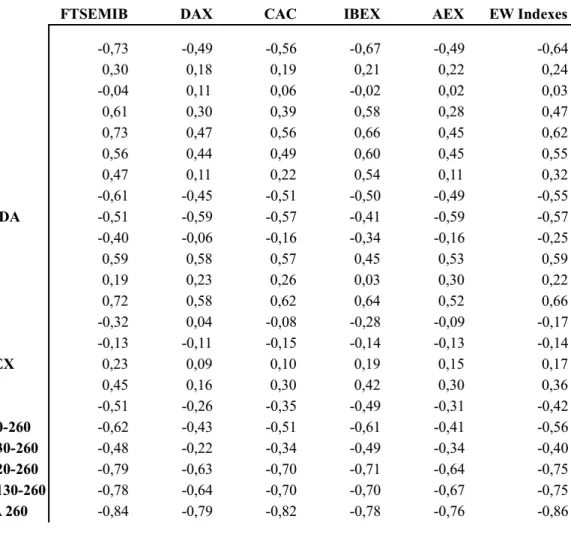
Table 7: Summary statistics for portfolio on combination of factors 36 Table 8: Returns portfolio produced by different deciles and quartiles 39 Table 9: Correlation of portfolio returns with trading strategies on

individual factors and stock indexes

41 Table 10: Correlation between indexes and trading strategies with

individual factor

42 Table 11: Result of four-factor model regression on portfolio returns 45

Table 12: Summary statistics for all portfolios 47

Table 13: Summary statistics portfolio formed with decile approach 49 Table 14: Result of four-factor model regressions on all portfolios

returns

50

Abstract

Previous research documented the existence of market anomalies; this work directs its focus on the possible usage of this evidence into a profitable trading strategy. It connects itself with the recent literature around the forecasting power of market anomalies over the cross-section of stock returns, in particular Lewellen (2014). Using a sample of twenty-six anomalies their pervasiveness is tested over the Eurozone (represented by the companies included in the five biggest stock indexes) in the new millennium era. A portfolio that combines the anomalies according to their past performance outperformed the main Euro stock indexes, obtaining a Sharpe ratio of 0,59 and an annualized alpha of 7,41%. Moreover the attractiveness of the portfolio is augmented by its dynamicity: due to the large amount of factors analyzed and the flexibility of the Sharpe Ratio as an indicator the portfolio is able to detect cyclicality in the economy and to wisely diversify around geographical areas.

Introduction

There has been evidence of the existence of market anomalies, variables that retain a certain forecasting power and allow an estimation of the expected stock returns. This proof does not grant certainty around the possible usage of the same variables in a profitable way. The main contribution of this thesis will be to extend the study of how an investor can use the findings around market anomalies, and then to assess how profitable this will turn out to be. Lewellen (2014) has already documented the predictive power of market anomalies in the US; I will extend this to the Eurozone. Secondly the contributions will be merely linked to the market and sample chosen: the efficiency of the euro market in the early 2000 will be tested coupled with an overview of how good the common asset pricing models capture the cross-section of returns.

Past models gave an explanation of how the stock price should be formed; according to the dividend discount model the value should be equal to the present value of all the cash flows that it pays. The capital gains produced by expected future price of the stock are incorporated by the present price, but these capital gains are mainly dependent on dividend forecasts at every point in time. A useful variation of this model, the constant-growth dividend discount model, relieves investors from making estimation of every dividend payments and introduces the constant growth of the dividends; this figure is hard to determine and it makes the analysis very sensitive.

Another model, the P/E model, asserts that the value of the stock should be decomposed in two parts: one it is linked to the present value of the company assets and their ability to generate cash flows, a second part is referred to the growth opportunities, represented by the present value of the projects that the company has. The price earnings ratio summarizes the information contained in these two parts, it reflects the market expectations around the growth opportunities of a company.

Even if extremely important, these models, as all models, have some assumptions that in practice make their implementation difficult; for example in the dividend discount model there is no clear way to estimate what is the growth rate of dividends, whereas for the P/E model the approximation of the NPV of future projects is also uncertain. Finally, both models

are using the risk-adjusted rate of return as discount rate, and this figure is always hard to appraise, even when using the current asset-pricing models.

In a broad way, it is this required rate of return, which is the objective of this work. This return should reflect the risk of the security and according to the efficient market hypothesis this risk is correctly priced such that there are no possibilities for investors to generate an expected rate of return, in excess to the risk-free rate, that it is not a risk premium.

Colliding to this view several exceptions were reported, i.e. market anomalies; these anomalies were the result of observations of the relation between the stock returns and different variables related to either the fundamentals of a company or its technical analysis. This study was usually conducted using the cross-section of stock returns with the anomaly variable significant in order to explain the differences in stock returns. More specifically the anomaly variable was discovered to have an explanatory power not recognized by known risk premiums, so a trading strategy based on the anomaly was able to produce abnormal returns, meaning returns not captured by the asset pricing model in use.

The existence of market anomalies created a whole new debate in the financial world related to their explanation: those certain about the efficiency of the market pointing the finger against the validity of the asset pricing models used, believing in their inability to capture all the risk premiums demanded by investors, and those convinced about the inefficiency of the market that see market anomalies as a clear example of it.

By now the progresses made are outstanding and despite the level of uncertainty still surrounding the topic both directions produced important results. On the one side several asset pricing models were developed with an increasing rationale (not based on empirical findings) and capability to explain the components of the stock return. On the other side the recent branch of finance named behavioral finance was able to explain several anomalies with behavioral responses that every investor is affected. The resolution of this debate is far from being solved and the present work does not want to interfere with it.

Indeed it is the usage of these market anomalies for profitable trading strategies that is the aim of this thesis. In fact the pure existence of the anomaly, even if proven by some study, does

not assure an investor about its efficacy in a trading strategy. This is because there are several biases that affect the validity of the discovery.

As pointed out by Hanna and Ready (2005) the anomaly might be an artifact produced by an intensive research over a database, this phenomenon is known as data snooping. Secondly the anomaly might be vanished due to its recognition by investors, this fact is also due to the increasing investing activity and the higher knowledge available to investors. Finally some market anomalies involve the usage of dynamic trading strategies that are extremely costly, then the overall gain produced by the strategy is basically nothing, entirely captured by the transaction costs that it requires.

Another relevant point is the fact that the anomalies may focus on companies in financial distress, as identified by Avramov, Chordia, Jostova and Philipov (2010) one set of anomalies is related to companies having high credit risk and deteriorating credit conditions, and another group of anomalies to companies having high credit risk but in a phase of recovery from recent financial distress.

Moreover the attention was more on how these anomalies are correlated with future returns, not on how the estimation of these returns according to the same variables are actually equal to the realized returns. The thorny point here deals with the ex-ante applicability of the trading strategy, a variable can be significant and have explanatory power but at the inception of the strategy this may not be known and predicted. In that case the practical implementation of the anomalies become relevant for an easy and tradable strategy. This work focuses on this and in particular on how to aggregate the anomaly variables into a portfolio.

Most of the academic literature is concentrated over the US market, to distinguish this work from the previous ones I decided to focus it on the Euro market; this will help to test the persistence of the anomalies in a market different from the one in which they were discovered. The dataset comprises companies in the five major stock indexes in the Euro area (France, Germany, Italy, Netherlands and Spain) and starts from the beginning of 2004 and it ends in the middle of 2014.

The usage of such database is important for two reasons: first it studies the persistency of market anomalies on companies that have a great market cap (and thus economically relevant)

then it makes the trading strategies liquid and tradable, avoiding the double bias of focusing on micro-cap stocks and companies in financial distress.

There are twenty-six variables analyzed and these include values and growth factors, size, momentum, and volatility. At first, for every variable an independent trading strategy is developed, with the application of each variable linked to previous findings around its relation to the average stock return. Every trading strategy is built on a market-neutral base and uses all the securities available (conditional on the availability of data for every factor); one of the goals was to limit as much the discretion around possible variants for every strategy, so the methodology around the construction of the trading strategy was clear and simple from the beginning.

The primary results will be linked to the aggregation and upcoming analysis of the variables into a portfolio. The aggregation discriminant will be the performance obtained by the strategies based on singular factors. The portfolio is tested out-of-sample since part of the dataset is used to have the performance and then, given this information, the strategies are set in place. In this step further variants, concerning different ways to sort stocks, will be used as robustness tests for the results produced by the portfolio.

Literature review

A comprehensive literature review of the topic has to start from its inception and so this revision starts from the CAPM initially introduced by Sharpe (1964), the CAPM was the first asset pricing model, a model that explains why the return of a security is different from another one. According to this model there is only one risk: the market risk. One of the main assumptions of the CAPM is that every investor holds a fraction of the market portfolio (which is the universe of all risky assets), benefitting from the diversification the contribution of a security to the overall riskiness of the portfolio is reduced to the interaction of the security with the portfolio. This interaction is represented by the market risk, the beta, which is proportional to the covariance of the returns of a specific security and the returns of the portfolio.

The CAPM represented the first attempt to give investors a general understanding of the differences in returns and risks of securities. It remained an unproven theory though since the introduction of the computers, which made possible to test the theory in practice and to see the actual degree of truth in explaining the differences across stock returns. The CAPM gave an explanation of the difference between stock returns, but it did not provide any clarification about the stock price development in the future and the extent to which this development can be forecasted.

An initial effort to give an answer to this problem was made by Louis Bachelier (1900) who observed the unpredictability of the stock price and affirmed its “random walk” behavior. Bachelier’s thesis did not receive much popularity at the time that was firstly published, nevertheless several economists recognized later its importance as a pioneering work in the field of financial mathematics. Kendall (1953) was one of the first economists to analyze the time series of prices in order to discover some kind of predictability and pattern in the series; confirming Bachelier’s intuitions he found that stock prices move in an unpredictable fashion, disregarding past performance.

This discovery was at first intended as a sign of market irrationality, then Fama in his PhD thesis used these findings to affirm the complete rationality and efficiency dominating the market. According to the efficient market hypothesis the information capable of affecting the stock price is already incorporated in it and so future price movements are basically random and unpredictable. The theory also suggests that once new and relevant information is disclosed the price will immediately adjust to a new level. Formally three sets of efficiency are highlighted by Fama: a weak form, in which just past information regarding the price is incorporated in the price, a semi-strong form, in which all the publicly information is included, and a strong form, in which also privately held information is included in the price; the semi-strong form includes also the weak form and similarly the strong form includes both, the semi-strong and the weak forms. These three versions of market efficiency can be tested, with most of the tests targeted to prove or reject the weak and semi-strong form, using technical (for the weak) and fundamental indicators (for the semi-strong). From another perspective EMH affirms the impossibility to generate any higher return that is not a result of the higher risk sustained, the impossibility to use the past information makes any abnormal return impossible; as a consequence this theory was not widely accepted on Wall Street.

These two theories together set the milestones for further research in the financial markets, this was mainly related to empirical studies aimed at the confirmation or rejection of the theories. With the computer era a massive quantity of data was analyzed and the financial markets were studied in a more quantitative way. A lot of trading strategies were performed using different variables, spanning all available information, and soon some of them produced abnormal returns, i.e. returns not explained by the CAPM; these variables were identified as market anomalies.

All of the empirical tests assume the form of joint tests of both theories, the EMH and the CAPM. If the joint test is accepted, implying no abnormal returns are present after the CAPM adjustment for risk, then both theories are proven, the asset pricing model and the efficiency of the market. If the test is rejected, it can be either because the market is inefficient or because the asset pricing model is not considering some feature that is relevant in the cross-section of stock returns.

Disregarding now the debate around the nature and explanation of these anomalies, it is provided a quick overview of the most well-known market anomalies, out of which some are included in the present research. As Fama and French (2008) underlined, two are the most used approaches to detect market anomalies in the cross-section of stock returns. The simplest one is to sort stock returns on the factor analyzed to see how the average return is distributed around the anomaly variable. The main advantage of this method is its simplicity and its ability to provide a quick overview of the impact of the factor on the stock return. A more technical approach involves the use of the Fama-MacBeth regression, divided in two steps, the first one involves time series regressions for all the assets in the portfolio, the stock return of each asset is regressed over the anomaly variable; in the second step all the coefficients estimated in the first one are used as independent variable in cross-sectional regressions using again the stock return as explained variable. This method provides a more quantitative description on how the factor analyzed is impacting the stock return and how it is priced in the cross-section of stock returns.

One of the first market anomaly discovered was the size effect, Banz (1981) showed that smaller firms tend to outperform bigger ones. Basu (1977) focused on the P/E ratio and observed that stocks with low P/E have higher returns than firms with high P/E. Stattman (1980) used the book value of equity to its market value, and documented the positive relation

between this variable and the stock return. Bhandari (1988) reported the positive effect of leverage on the average stock return. Loughran and Ritter (1995) showed the negative performance of companies that experienced an IPO or seasoned equity offer in the five years after the operation. Titman, Wei and Xie (2004) noticed how companies that invest more tend to have negative abnormal returns, this finding is even augmented for those companies with higher cash flows and more solid capital structure. On a similar level Cooper, Gulen and Schill (2009) documented how firms with low asset growth (measured as the yearly change in the total assets) tend to outperform firms with high asset growth. Sloan (1996) identified the negative impact of accruals on the stock price. Pontiff and Woodgate (2008) confirm findings around the positive link between long-term stock return and share repurchase announcements, stock mergers and seasoned equity offers, exploring the relation of stock issuance and the cross-section of stock returns, affirming how stock issuance is statistically more relevant in predicting returns than other well-known anomalies.

A special mention is appropriate for those anomalies that are based on the historical stock prices; this because out of the market anomalies those are the ones that contradict even with the weak form of the EMH. One of the first paper using technical indicators is the one from De Bondt and Thaler (1985), using the past three and five years stock performance they observed the stock reversal effect, meaning that the companies that performed worst were the ones that outperformed the others in the subsequent period, simultaneously the best ones underperformed the others. A similar conclusion was found by Jegadeesh (1990), who showed the negative auto-correlation of returns in the 1-month window but also the positive auto-correlation for longer lags up to one year. Moving from this last finding, Jegadeesh and Titman (1993) used the stock returns over the past three to twelve months (skipping the most recent week to avoid the negative correlation in the stock returns) and observed how the past winners outperformed the past losers also in the future, this particular anomaly gained much recognition and it was named momentum.

An interesting implication of the EMH is that whenever new information is released the stock price should immediately adjust reflecting the content of the information. This gave rise to a whole new type of study in finance, the event study, an analysis directed to understand the development of the stock price on certain event like an earnings announcement. Despite their relevance, Ball and Brown (1968) found that there are no price adjustments after an earnings announcement. Rendleman, Jones and Latané (1982) studied the phenomenon in a different

way, instead of looking at the earnings announcement they observed the earnings surprise (measured as the difference between the estimated/expected earnings and the announced one) and observed not only a price adjustment but also a momentum pattern whenever the surprise was positive or negative.

The interpretation of these market anomalies is always arduous, sometimes because it is puzzling to find a rational explanation for the anomaly, in other words it appears to be difficult to explain the superior returns as a compensation for the higher risk sustained. Even if the previous statement is correct for factors like P/E or size is really hard to think that the problem is related to the overall efficiency of the market; such that strategies based on such factor are too simple to be able to produce abnormal returns, investors in the world should do this on regular basis and then the abnormal return should disappear.

Fama and French (1996) argued that for some anomalies the factor used to obtain the abnormal returns may act as a proxy for a different source of risk; for example when looking at firms with high book to market ratio they observed how these companies are usually more unstable and more likely to be in financial distress, a similar consideration is done for small firms, which are more prone to suffer variations in the business cycle.

Different asset pricing models were developed in order to explain and capture the cross-section of the returns in a more comprehensive way than what the CAPM did. Some others indeed argued that the presence of market anomalies is a distinct sign of the market inefficiency, and within this line of thought some think that this is because the market is dominated by irrational investors and that modern finance ignores some behavioral effects that are able to explain most of this irrationality.

The first asset pricing model that tries to solve this issues is the one developed by Fama and French (1992), in this model along with the market beta also a size and value factor, represented by B/M, are added. The reasons for having this three factors is mostly empirical, given the previous findings Fama and French decided to expand the CAPM with two of the most constant market anomalies. The result is surprisingly good with the model that seems to capture the cross-section of returns for the US market from 1963 to 1990. The surprising part was though related to the poor significance of the market beta, with the size and value coefficient that were basically the only explanatory variables for the returns.

With the three-factor model most of the anomalies vanished, but one of the most important, momentum, still persisted. In order to include this variable Carhart (1997) added a momentum factor, similar to the three-factor model also the four-factor model is an empirical model, it takes as given some findings that are relevant in the cross-section of returns and it includes those in the model.

Recently Chen, Novy-Marx and Zhang (2010) developed an alternative three-factor model, this model is constituted by three explanatory variables: the market beta, an investment factor and a profitability factor (with ROA used as proxy). The introduction of these two factors is motivated by an investment reason. To infer the cost of capital (i.e. the required return demanded by investors) the level of investments is meaningful: assuming a fixed level of expected cash flows, the cost of capital determines the NPV of a project, if high the level of investment will also be high because of the profitable project to finance; the opposite is also true. So from the level of investment one can infer the cost of capital of the company; this measure is coupled with ROA. Observing a high ROA and a low level of investment means that the high ROA is offset by a high cost of capital; ROA in this sense acts like another determinant for the specification of the cost of capital.

Of all the anomalies, momentum (together with other technical factors) is one of the most deceptive and hard to explain, an attempt to solve the problem was made by Chen (1991) who gave the interpretation of momentum as a pattern emerging because risk premiums are time varying. The level of risk and risk aversion are both changing during business cycles, e.g. during a recession expected returns can be higher because of an increase in risk and risk aversion (since wealth is decreasing and we face diminishing marginal utility function). To the extent that these cycles happen with a certain frequency this can lead to the technical pattern in the stock returns, as momentum.

On a similar level, Campbell et al. (2008) declare that the size and value factors on the three-factor-model are acting as an imprecise proxy for the risk of the firm being in financial distress, this because companies having high loadings on these two factors are exhibiting high risk but not high returns. Confirming the result of this paper Avramov, Chordia, Jostova and Philipov (2010) explore commonalities across the anomalies and noted how most of them are highly related to companies being in financial distress or recovering by it. Hence they

conclude that most of market anomalies are generating abnormal returns because of the inability of asset pricing models to capture the risk of financial distress.

Liew and Vassalou (2000) used portfolios based on size and B/M and found how the returns produced by these portfolios can be linked to macroeconomic risk. The main result of the paper is that these two factors have explanatory power when regressed over future GDP growth, even when controlling for other known predictors of business cycles. This result suggests that small and high B/M companies are more prone to be in financial distress when an economic downturn is approaching. The intuition is stronger because of the high persistency for companies to have either small market cap or high B/M, suggesting that investors are aware of this risk and then demand a premium for holding such stocks.

In their latest paper Fama and French (2013) developed a five-factor model, with the goal to expand the explanatory power of the three-factor model and to base this more on a rational base rather than an empirical one. They noticed how size, B/M, expected earnings and investment are all variables that are implied and included in the dividend discount model; an important model aimed to identify the intrinsic value of a stock, in the model is asserted that this value is the present value of the future dividends that the stock will pay. One of the practical issues was to find a valid proxy for profitability and investments, they then used operating profitability minus interest expense for profitability and the asset growth for investment. The model failed the GRS test, that measures if the levels of the intercept from a multiple regression model are jointly zero, nevertheless it provides a good explanation of the cross-section of returns. Interestingly, the B/M factor is not relevant in order to capture abnormal returns, because its significance is seized by the other four factors, but still it provides a good explanation of portfolio’s exposure towards the size, value, profitability and investment.

Despite the growing explanatory power of such asset pricing models some academics are convinced about the irrationality and inefficiency of the market. Kahneman and Tversky (1979) in their prospect theory used tools from psychology to explain the behavior of investors, in particular they stated how an investor does not act rationally and does not make optimal decisions, instead it is biased from a series of behavioral phenomena. In their paper they enumerate three common patterns in investors’ behavior: the framing effect, stating that the context in which the individual makes a choice is relevant for the outcome of this

decision; the loss aversion, affirming the fact that a loss is always worse than sacrifice a gain; the isolation effect, when facing consecutive probabilities individuals tend to isolate the odd of each event without considering the overall probability.

This whole branch of study got the name of behavioral finance and it is based on two pillars: first economic agents are believed to act irrationally and secondly rational arbitrageurs cannot exploit the mispricing because of limited resources. In addition to this the arbitrage opportunities are not of the pure arbitrage nature, i.e. they are not risk free, mentioning a common sentence attributed to Keynes: “markets can stay irrational longer than you staying solvent”.

One of the most important papers in this area, by De Bondt and Thaler (1994) explained the anomalies related to some value factors (P/E for example) as under or overreactions of investors, in particular when new information is released the market participants tend to exaggerate the feelings toward a company. This explanation rapidly gained consensus and different papers after this tried to expand the initial definition, for example La Porta (1996) argued that analysts are always too optimistic or too pessimistic when giving expectations about firms’ growth rates and this gives rise to mispricing in the market.

According to Grinblatt and Han (2002) one anomaly, stock reversal in the short term, can be explained with the disposition effect, according to this investors are less likely to recognize losses than gain, so the consequence is that they will keep stocks that are underperforming and they will sell those that increased in value to lock the gains.

The critics of behavioral finance argue that it is easy to explain a market anomaly with a behavioral response when it is done after having observed the anomaly but impossible to use the same argumentations to detect it.

The present work focuses on the usages of the previous findings related to market anomalies, its primary aim is to see if these anomalies can lead to substantial profits and how can they be interpolated with each other to maximize the return. This goal will be coupled with the intent of finding what could have been possible and rational ex-ante, by this it is meant that the trading strategies are performed out of sample, with a precise method (i.e. limiting as much as possible discretionary choices) to use the information available.

There are several papers that share a similar aim, at first, Fama and French (2008) published a paper in which they revisited all the principal market anomalies with the purpose to understand which ones are the most persistent and how are they structured in different size groups. They use both portfolio sorting and cross-section regression to have a clear picture of which factor is relevant in order to explain the stock returns. The size division has to be intended for a reason of economic significance: even if they account for 3% of the total capitalization microcaps stocks are 60% of the number of stocks in the NYSE-Amex-NASDAQ universe and according to Fama and French 60% of the stocks in the extreme portfolio sorting are from microcap stocks. Having divided stocks into three size groups (micro, small and big) they found that returns associated with net stock issues, accruals and momentum are the only widespread in each group.

Haugen and Baker (1996) started their analysis with the consideration that non-risk related factors are relevant explaining the stock returns, assuming that also stocks are different in their liquidity they divided factors in five classes: risk, liquidity, price-level, growth potential and price history. They used cross-sectional regressions to estimate the expected return for the following month using all the factors available (a total of fifty variables), the payoffs are aggregated with a simple average of the past twelve months reaching the expected return for the factor analyzed. The first twelve months prior 1979 are used to make a first estimation of the payoffs, the future coefficients for each payoff are then given by a 12-month trailing mean, the whole process is repeated till the end of 1993. Together with a test with all factors other two are run to see if the results are highly dependent to the effect of some previously mentioned anomaly: first all factor besides momentum related ones are dropped, then all except the ones related to the cheapness in price (for instance B/M and P/E). The spread between the realized returns from the highest to the lowest decile is 35% and this spread is drastically decreasing when the factors are simply momentum or cheapness in price ones, the authors’ deduction is that the predictive power is laying mostly on the multitude of factors used. The main results of the paper are linked to the average fundamentals of companies that are in the highest decile from the ones in the lowest one; Haugen and Baker looking at these features are trying to infer if the superior performance of decile ten is a reward for the highest risk taken. The assessment is made in two ways, at first looking at the average fundamentals across deciles, like D/E or volatility, the second using the Fama, French three-factor model. The conclusion is that it is quite difficult to argue that firms in decile ten are riskier than the ones in the lowest decile, looking at the fundamentals these companies show a more stable

condition and lower volatility, regarding the model they have lower loadings on all three factors.

Hanna and Ready (2005) reexamined some of the previous findings related to market anomalies and questioned whether a dynamic trading strategy combining these anomalies would lead to substantial profits, even adjusting for transaction costs. The anomalies (B/M, six months past returns, Haugen and Baker’s factors) are organized in different independent portfolios, using the same dataset (the Russell 3000 Index) but on a more extended period to the papers related to the anomalies (from 1979 to 2001) so the strategies are partially tested out-of-sample. Stocks are assigned decile rankings for each factor; for B/M and momentum the sort is done directly from the factor, whereas for the Haugen and Baker’s variables the sort is done by the expected returns. The portfolios are formed using companies in decile one and ten; both equally-weighted and value-weighted, with monthly rebalancing (important to account for the transaction costs). For every strategy there is a difference in return from decile ten to decile one, with the Haugen and Baker’s difference more than double than the other two portfolios (+31,2% and -6% the annualized return); this result is statistically significant different from zero at the .01 confidence level using the t-test. The excess return of each strategy is then tested using the CAPM, in order to see which weight to give for every strategy, the alpha is divided by the residual variance. Also accounting for trade delays and transaction costs the portfolio formed on B/M is the one showing the best alpha/residual variance ratio The last part of the paper concerns the portfolio optimization, to maximize the Sharpe ratio. This maximization is unfeasible in practice because it takes the ex-post distribution of the returns as given, having this in mind the optimal portfolio when only long positions are allowed is made 80% by B/M portfolio and 20% of the momentum portfolio. When short selling is permitted the HB portfolio is in the optimal one just for the short part, even excluding it the overall result doesn’t change much (Sharpe ratio of 0,38 versus 0,378). Lewellen (2014) focused on the Fama-MacBeth regression to forecast returns; using a set of fifteen firm characteristics for the US stock market from 1964 to 2009, Lewellen, in his primary test, used the slopes derived from a rolling ten years FM regression in order to predict monthly returns. These fifteen factors are organized in three different portfolios, with the most persistent factors composing the first model (like B/M or size) and the less persistent factors added to this first set in the second and third portfolio; the reason is to move from a portfolio of well-known predictors of stock returns from others that include other variables

that an investor could have thought of. Stocks are then sorted on the expected return forecast. The main result concerns the overall realized return versus the forecasted one, for the first portfolio the estimated spread between the top and worst decile is 2,82% whereas the realized one is almost as large, 2,43%. The interesting result is that the forecasting power of the most important factors account for most of the success of the FM regression, in fact the last portfolio, including factors like dividend yield and sales to price ratio, does not add anything to the overall forecasting power of the model.

Following this last stream of literature I will move from analyzing the predictive power of market anomalies to the employment of the same variables in different trading strategies, trying to detect how much an investor could gain from this evidence. My effort will be concentrated on how these factors can be aggregated into a profitable and ex-ante feasible strategy. Differing from these papers I will not use cross-sectional regressions to determine the expected returns but a more practical approach, directly developing a trading strategy based on those variables. The analysis starts with the factors taken individually rather than having all of them in a portfolio; as a consequence the following step is their aggregation, rather than separation, into a portfolio. The discriminant for the aggregation will be the actual performance of every factor and not a division “per classes” as in Lewellen (2014) or Haugen and Baker (1996).

One of the main criticism related to market anomalies is the usage of the same database (US market generally) to discover and test the magnitude of the anomalies, the phenomenon is known as data snooping. Expressing this concept in the words of Ronald Coase: “if you torture the data long enough, it will confess”. Some work has been done to avoid this bias and even if not widespread to all findings around market anomalies at least the most important ones were also tested using financial markets different from the US one.

Asness, Moskowitz and Pedersen (2013) extended the evidence over momentum and value in the British, European and Japanese markets; finding abnormal returns that are consistent with what documented for the US market. Using also different and uncorrelated asset classes a similar patter is discovered, since the strategies based on momentum and value have a strong correlation structure this induces the authors to conclude that momentum and value might be a premium for global risk factors.

Fama and French (2012) find a considerable persistency of size, value and momentum effects in international stock markets (North American, Europe, Japan and Asia Pacific). Using different versions of the three-factor model and the four-factor model Fama and French tried to explain the returns produced by trading strategies on size, value and momentum for each of the region; when the explanatory variables (meaning the returns produced by the factors of the asset pricing model) are taken globally the results are quite poor, contrasting partially with Asness et al. (2013) and the possibility that size, value and momentum could be linked to global risk factors.

The contributions that I am expecting will be twofold, even though very linked to each other. On one side the different data set from the original one, in which the market anomaly was discovered, acts as a double check for the persistence of the anomaly. In addition the different period analyzed adds ulterior material for this proof. On the other side studying the implementation in practice of market anomalies will function as a verification of them on a different level: even if present the anomaly could not be used because at the beginning of the period the investors do not have any tool to infer how much predictive power each variable has. Both contributions are acting in the more comprehensive environment of the efficient market hypothesis, as all these studies the main conclusion will always be related to the possibility or no to use available information to spot mispricing in the market that can lead to abnormal returns.

Data

The analysis is directed towards the Euro market; instead of picking a broad index as the EURO STOXX I preferred to create a sample of companies from the five most important Euro stock market indexes; namely the Dutch (AEX 25), French (CAC 40), German (DAX 30), Italian (FTSE MIB 35) and Spanish (IBEX 35). The complete list of companies used is presented in the appendix.

Following Fama, French (2008) I use only the bigger stocks. In fact this is what institutions actually invest in, among other things, because of liquidity concerns. As a proof of this, around all the minimum points touched by the market caps of all companies in the whole

sample the median point is 3.351 billion €, just as a comparison Fama and French in the same paper identified 610 million $ the breakpoint on the NYSE to be a micro-cap stock.

The set of factors analyzed are related to previous findings surrounding their applicability to predict stock returns in the cross-section; trying to gather an acceptable number of companies reporting, the list of these factors can be found in the appendix. Broadly speaking the factors covered are mostly related to the fundamental variables of a company, highlighting different aspects from the risk, profitability or fair valuation of the stock price, but also technical indicators based on previous stock returns.

Table 1 provides an overview of the factors and the descriptive statistic for the whole sample and the two sub samples. The period analyzed is from 2004 to mid 2014. The data is initially daily organized and from this the technical factors are built. All the data, from the price series to the accounting variables is downloaded from Bloomberg. Price series is retrieved using the PX_LAST ticker, which gives back the closing price of a specific day. Accounting variables are, on the other hand, linked to company reports.

More precisely the technical factors used can be divided into three categories: momentum, volatility and market beta. Momentum consists of the cumulative return of the past 20-260 and 130-260 trading days; using the same windows but the average return instead of the cumulative one other two factors are created. Similarly, volatility comprises two factors constructed using the standard deviation of the past 20-260 and 130-260 daily stock returns. Finally the market beta refers to one factor that is the slope of past 260 daily stock returns of a security and the return of the stock index in which the company is quoted on.

In order to avoid the problem of analyzing a period taking the ex-post winners (i.e. survivorship bias) the index composition is taken at the inception of the strategy. The list of companies forming the indexes is assembled again in 2009, this is necessary because some companies got delisted through time and to successfully perform the strategies I need a substantial number of companies that are alive and disclosing information. Some companies are quoted in more than one market, to not have the same security twice the stock listed in the peripheral market is deleted; these companies are just two for the 2004 index and three for the 2009 one.

A clarification: most of the companies are always reporting, but for some factors the availability is not so widespread and this is an issue with the factor itself and not with the fact that the company is not reporting at all. When a company is delisted in the trading strategy this acts in the same way as a real event and not like an ex-post manipulation; the company is available for investment purpose until the moment that it gets delisted.

Table1: descriptive statistics 2004-2014.

All the data is gathered from Bloomberg, for each factor is reported the average value (Avg), the standard deviation of the average value (Std) and the sample size (N).

Methodology

Given a set of proven predictors in the cross-section of stock returns, the problem is to find a profitable way to use them. Instead of using cross-sectional regressions to see to what extent each factor predicts the stock return and then make usage of this information I directly used all factors individually into trading strategies and then valued their quality based on the performance obtained.

Since daily trading would be too costly transaction wise, I extracted the data at the end of every month from the database and built all the trading strategies that are rebalanced monthly. More specifically the signal to buy or sell is given at the end of a month and then applied for the following one. This method partially differentiate this work to ones that share the same aim, mostly Lewellen (2014) and Haugen and Baker (1996), because it takes factors individually and then mixes them rather than initially start with a considerable amount of factors and then excluding some. This approach is different because it ignores the correlation between factors relying solely on the goodness of their past performance.

To not develop the strategies on information that is not yet available a lag is introduced, there is a distinction between variables though; the information regarding fundamental variables is lagged by three months due to the delay of companies to release the annual and infra annual reports. Whereas no lag is applied concerning market information since these are assumed to be easily accessible by everyone and basically at every moment.

The allocation of resources is achieved through portfolio sorting, using ranks. Specifically every security receives a rank established on the factor examined, the long position is selected using previous findings around the factors, e.g. for ROA the company displaying the highest ROA will also have the highest rank. For some factors the link is immediate since the factor is the same variable analyzed in some previous paper, for others there is no such link, I then tried to apply the intuition of the paper to the new factor.

Instead of looking at the different percentiles and select a top/worst class in which to invest in, I preferred to use the whole sample, assigning a weight based on the rank for all. At first this eliminates the discretion among the percentile to pick when an investment decision is made, i.e. there is no model that states before which percentile is better to use, so this choice is left to the preference of the investor. Then it will help to see the persistency of the anomaly variable not only in the extremes of the portfolio sorting, but using all the securities available. Roughly, at every point in time, half of the companies will compose the long position and the other half the short position.

The strategy is built on a euro-neutral base and standardized such that the long position sums up to 1 and the short position to -1. The weight given to each security is applied following the approach of Asness, Moskowitz and Pedersen (2013):

𝑤_!"! _{= 𝑟𝑎𝑛𝑘 𝑆} !" −  

(𝑁!+  1

2 )

𝑐_!

Where N represents the number of companies, i the company, t the time and S the factor used, c is a scaling factor:

𝑓𝑜𝑟  𝑎𝑙𝑙  𝑙𝑜𝑛𝑔  𝑝𝑜𝑠𝑖𝑡𝑖𝑜𝑛𝑠:  𝑐_! =   𝑟𝑎𝑛𝑘 𝑆_!" −  𝑁!+  1 2

!

At the end of this procedure I have a trading strategy for every variable in the dataset; the overview of the risk-return profile for all the individual strategies is presented in table 2. As a matter of completeness in the table are also presented all the five stock indexes plus an equal-weight composition of the five.

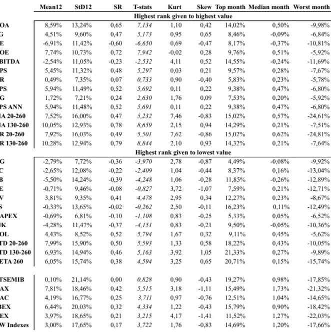
Table 2: summary statistics for trading strategies on singular factor, from May 2004 to May 2014.

In the first set of factors the long position is assigned to those securities having the highest values, in the second set the opposite is done. The index returns in the last panel are total returns, in excess to the risk-free rate. Momentum factors are constructed using moving averages and cumulative returns.

Last remark: in table 2, I highlighted the Sharpe ratio which in this case is not considering the excess risk premium but just divides the mean with the standard deviation, this is because the strategies are constructed on a cash neutral base and so the risk-free rate can be ignored.

Results

Support the evidence: abnormal returns for the twenty-six factors

Before going through the analysis of the factors and their employment into a composite trading strategy it is worth to first test the results of the simple trading strategies on singular factors. This will provide the preliminary results around the persistency of these anomalies over the new period and, more importantly, a new market.

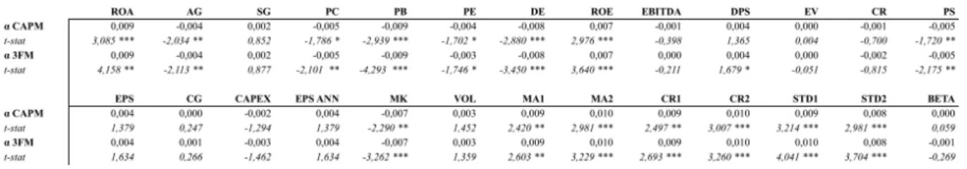
Table 3: alphas for trading strategies on singular factors, returns from May 2004 to May 2014. * indicates statistical significance at the 10% level **=5% level and *** at the 1% level.

The models used to observe the alphas are the ones mostly used in the papers where the anomaly was discovered. Even if a more complete model could be used this choice is prevalently linked to the interest of observing the anomaly in a different context with the same instruments. In table 3 it is provided evidence of the abnormal returns produced by the strategies, the coefficients are not highlighted since when further processing the variables into a portfolio they are not considered.

Despite the usage of the same variables as in related papers, a major difference could be the different methodology used to build the trading strategies, once again, not investing just in the top-worst decile but in all the securities with a weight proportional to the rank.

Table 3 depicts a controversial scenario: out of twenty-six factors thirteen obtained a positive alpha according to both asset pricing models, and from this group eight are statistically significant; even if the group represents the majority of the variables it is still not high enough to conclude that the market anomalies are mostly pervasive in the Eurozone. It should also be noticed that in the same group several factors are very similar to each other (for example the variants of momentum or volatility).

It is also true to affirm that not even the most well-known ones are present in Europe; starting with P/B the alpha is not just negative but also highly significant even when correcting for the Fama French three-factor-model. A similar situation is displayed by asset growth, a variable that is used as a proxy of investments in the new five-factor-model of Fama and French (2013). D/E also represents an important contradiction to the evidence, firm that showed a lower leverage actually gained a premium that is hardly explainable as risk premium as it is indeed the high leverage since it can be easily linked to the likelihood of a firm to be in financial distress or more vulnerable if a recession is approaching.

From the group of variables that exhibited a negative alpha MK is one of the most evident example. Big stocks outperformed small stocks, and generated a positive abnormal return, statistically significant at the 10% level for CAPM and 1% for the three-factor-model. Indeed it should be mentioned that most of the American literature considers bigger indexes, like the Russell 3000, and so the spanning market cap is more accentuated that the one I have in my sample; so this difference can partially explain the different result.

It is most likely, though, that the difference is rooted in the sample, and this consideration is valid for all the anomalies; some anomalies may not be pervasive because of the distressed period analyzed, so the bad performance can be partially tied to this and the fact that these strategies are cyclical rather than that they are not applicable to the Eurozone market. Going back again on size and value, because of their popularity among the anomalies, it should be noticed that the poor result that they obtained during this period is also clearly shown in the returns of the SML and HML factors of the three-factor model for Europe.

Moreover, anomalies are usually discovered using an extended period, since this study uses a 10-year period the pervasiveness of the anomalies can be rejected for sure for the period considered but since this is not tremendously high their presence in the Eurozone cannot be fully assessed.

Afterwards, when correcting for common risk factors, I will use a more complete asset pricing model, the four-factor-model. Consequently, the alphas of the individual strategies will be lower (especially the ones related to momentum and profitability, so the ones having the highest alphas).

Factors aggregation: Sharpe ratio’s screening

The considerations around the results obtained by each individual strategy will come together with the ones obtained by the portfolio made by combination of factors.

The idea of aggregating the factors is linked to the belief that the performance will improve because of the higher degree of information used and taken advantage of; in other words it introduces the benefits of diversification. The problematic point copes with the aggregation of the factors, meaning to have a rationale for having a particular set of factors together.

Since one of the goal is to leave as much of the heterogeneity around investors’ beliefs and preferences out, instead of aggregating factors using an artificial division by classes I used their past performances. The tool used to build the different portfolios is the Sharpe ratio produced by the strategies based on singular factors. This indicator is chosen because it summarizes the information regarding the risk-return profile of a particular strategy and mostly, it makes every strategy comparable and easily classified. A higher Sharpe ratio, even if produced by a strategy that has a low average return, is always preferable to a lower one with a high average return because of the possibility to leverage the first strategy and magnify the returns.

In order to have a stable outlook of the Sharpe ratios, the first twenty-four months of the sample are used to observe the development of this figure and used to invest from month twenty-five (April 2006) onwards. When I am calculation the Sharpe ratio I always use all the history available, such that the sample used for this computation is enlarged every month by one unit.

Technically the trading strategy is performed using the same rules as before, the difference is now that the rank is not a direct product of the factor but is a combined rank, having each factor weighted differently according to their Sharpe ratio. For every security i, the formula to obtain the ranks later used to sort the securities is the following:

𝑅𝑎𝑛𝑘(𝐹_!") =   𝑤_!∙ 𝑅𝑎𝑛𝑘(𝑆_!")

!"

!!!

To not have in the portfolio two identical factors I discarded the EPS annualized factor and the two momentum factors with moving averages. This because in the first twenty-four months they performed slightly worse than their counterparts, respectively the trail 12-months EPS and momentum factors built using cumulative returns.

In view of the fact that the factors suffer from different number of observations I adopted the same approach as in Haugen and Baker (1996). I modified the database so to have all factors with the same amount of observations: when the company is alive but a certain factor is missing the mean sample value is assigned to that company. The aim is not to throw away valid data reducing the sample to companies having all factors. Nonetheless this step may bias the accuracy of the results, this is certainly true for those factors that exhibit a serious lack of data but in general this is not the case, having most of the factors with quite equal observations (close to the totality of companies).

Since investors care more about the performance and less about what past academic evidence have proved I took a similar point of view, treating all the variables in an equal way, using the Sharpe ratio that they produced as the only discriminant. This consideration then induces to include the factors that underperformed and question if the long position was chosen wrongly, i.e. the factor was showing an opposite relation to returns than the one initially thought. Using the past performance as only driver to aggregate the factors has a main downside: it ignores the correlation between the factors. In fact it might happen that most of the portfolio’s returns are resting on variables that are positively correlated with each other. The risk is that the portfolio could be more vulnerable to sudden changes in the profitability of the same variables; in other words it looses in terms of diversification.

A simple way to aggregate the factors moves from the consideration that the ones having the highest Sharpe would be the factors most attractive to use; then using a formula to give a weight to the factor that is proportional to its Sharpe ratio should reflect this consideration. A possible procedure to do it would be to simply divide the individual Sharpe by the sum of all the Sharpe ratios of the strategies:

𝑤_! =   𝑆! 𝑆_!

!

In this view factors are observed for their absolute Sharpe ratio value: if the sign is positive it means that the relation is the one initially assumed and if it is negative it means that the ranking may be given incorrectly and should be changed into the new order (e.g. instead of sorting stocks using a descending order sort them in an ascending one). Expanding this idea, if the Sharpe ratio is negative an investor could have thought about the misuse of a factor and that if he had invested following an inverted order he would have got a positive ratio. In this case this presumption is certainly true because the specific formula that gives weight to securities assures that if the highest rank would be given to the lowest value instead of the highest the return would be the same as before but with a different sign. Therefore the Sharpe would be the same in absolute terms but with a plus instead of a minus in front.

At first glimpse changing the belief towards a factor just because the Sharpe ratio is negative may be too drastic, but it should not be forgotten that the metric is built from, at least, the past twenty-four months performance and so it should capture something more than a pure deviation from the relation expected. Even if the previous statement is true this will not compromise the results of the portfolio: if the Sharpe ratio changes from positive to negative in a specific month it is fair to assume that it was close to zero until the month before. Therefore the factor will receive, in both, previous and current portfolio rebalancing a weight that is very low.

Table 4 reports the results of this portfolio, it is useful to have a first idea around its performance. The risk-return profile obtained was above the five indexes that act as a benchmark; the average return was above the one offered by the indexes and the volatility was slightly lower. The cumulative return of the strategy denotes a clear upward trend, with most of the returns that are coming from the after crisis period.

Table 4: summary statistics for portfolio created using all the 23 variables. The starting point is May 2006 and it goes till May 2014.

Figure 1: cumulative return of the portfolio, from May 2006 to May 2014.

I will now focus on the interpretation and further analysis of the results earned by the simple strategies and for the portfolio on all factors. Given the fact that the effect of the financial crisis of 2008 in this sample is really relevant and due to the shortness of the period analyzed, I will provide a separate picture for its effects on the trading strategies.

Data Analysis

Interpretation: strategies on singular factors

From the evolution of the average monthly return obtained by each strategy some considerations can be made around the factors and their relation to the realized returns. I highlight now the most evident trend in this matter. A graph in this sense would be clearer and more efficient than words, in figure 1 all the individual strategies’ average monthly returns are displayed.

0.00%   25.00%   50.00%   75.00%   100.00%   125.00%   150.00%   Ju n-­‐0 6   O ct -­‐0 6   Fe b-­‐0 7   Ju n-­‐0 7   O ct -­‐0 7   Fe b-­‐0 8   Ju n-­‐0 8   O ct -­‐0 8   Fe b-­‐0 9   Ju n-­‐0 9   O ct -­‐0 9   Fe b-­‐1 0   Ju n-­‐1 0   O ct -­‐1 0   Fe b-­‐1 1   Ju n-­‐1 1   O ct -­‐1 1   Fe b-­‐1 2   Ju n-­‐1 2   O ct -­‐1 2   Fe b-­‐1 3   Ju n-­‐1 3   O ct -­‐1 3   Fe b-­‐1 4   All  factors  

Figure 2: average monthly return (from month 24) for all 23 factors. -­‐0.20%   0.00%   0.20%   0.40%   0.60%   0.80%   1.00%   1.20%   1.40%   Ap r-­‐0 6   Au g-­‐0 6   D ec -­‐0 6   Ap r-­‐0 7   Au g-­‐0 7   D ec -­‐0 7   Ap r-­‐0 8   Au g-­‐0 8   D ec -­‐0 8   Ap r-­‐0 9   Au g-­‐0 9   D ec -­‐0 9   Ap r-­‐1 0   Au g-­‐1 0   D ec -­‐1 0   Ap r-­‐1 1   Au g-­‐1 1   D ec -­‐1 1   Ap r-­‐1 2   Au g-­‐1 2   D ec -­‐1 2   Ap r-­‐1 3   Au g-­‐1 3   D ec -­‐1 3   Ap r-­‐1 4   VOL   CR1   CR2   STD1   STD2   BETA   -­‐1.00%   -­‐0.50%   0.00%   0.50%   1.00%   1.50%   Ap r-­‐0 6   Ju l-­‐0 6   O ct -­‐0 6   Ja n-­‐0 7   Ap r-­‐0 7   Ju l-­‐0 7   O ct -­‐0 7   Ja n-­‐0 8   Ap r-­‐0 8   Ju l-­‐0 8   O ct -­‐0 8   Ja n-­‐0 9   Ap r-­‐0 9   Ju l-­‐0 9   O ct -­‐0 9   Ja n-­‐1 0   Ap r-­‐1 0   Ju l-­‐1 0   O ct -­‐1 0   Ja n-­‐1 1   Ap r-­‐1 1   Ju l-­‐1 1   O ct -­‐1 1   Ja n-­‐1 2   Ap r-­‐1 2   Ju l-­‐1 2   O ct -­‐1 2   Ja n-­‐1 3   Ap r-­‐1 3   Ju l-­‐1 3   O ct -­‐1 3   Ja n-­‐1 4   Ap r-­‐1 4  

ROA   DE   ROE   EBITDA   DPS   EV  

-­‐1.00%   -­‐0.80%   -­‐0.60%   -­‐0.40%   -­‐0.20%   0.00%   0.20%   0.40%   0.60%   0.80%   1.00%   1.20%   Ap r-­‐0 6   Au g-­‐0 6   D ec -­‐0 6   Ap r-­‐0 7   Au g-­‐0 7   D ec -­‐0 7   Ap r-­‐0 8   Au g-­‐0 8   D ec -­‐0 8   Ap r-­‐0 9   Au g-­‐0 9   D ec -­‐0 9   Ap r-­‐1 0   Au g-­‐1 0   D ec -­‐1 0   Ap r-­‐1 1   Au g-­‐1 1   D ec -­‐1 1   Ap r-­‐1 2   Au g-­‐1 2   D ec -­‐1 2   Ap r-­‐1 3   Au g-­‐1 3   D ec -­‐1 3   Ap r-­‐1 4   AG   SG   PC   PB   PE   PS  

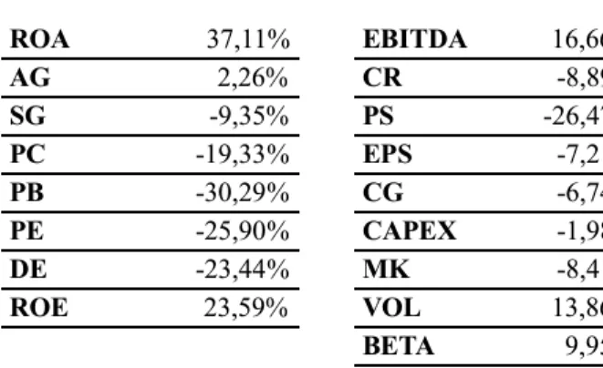
At first not many factors had a stable pattern over time, one of the causes could be the impact of the crisis and its effects that were able to change the entire trend showed until that moment. Out of twenty-three factors eleven had a positive average monthly return, in line with the past evidence, for at least 90% of the months. From this group of twenty-three factors profitability factors, ROA and ROE, DPS, both momentum factors, volatility and earnings-per-share are included.

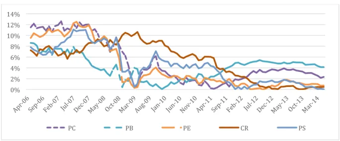
One of the most recent anomalies, asset growth, did not confirm any negative relation with the stock return, having the strategy going long on low asset growth companies two-thirds of the times a negative average return. Another variable EBITDA/Sales that, in theory, should be similar to a profitability indicator, highlighting how good a firm is doing in managing the operative costs, produced a very poor performance in the sample analyzed. Most of the factors related to the fairness in pricing exhibited a negative trend, meaning that from mid 2006 they were producing good performance but from that had a constant decline, with the inception of the crisis culminated in negative results. Linking to this, again the crisis had a disrupting effect for most of the strategies, for some changing the trend from positive to negative, for some other representing the main source of gain.

It is hard to find a general explanation for these changes in the performances when looking at factors individually, but when aggregating them into groups some useful considerations can be made. Out of the group of strategies that lost a lot, D/E, MK and P/B changed drastically their trend with the abruption of the crisis; the preference from small and leveraged firms

-­‐1.00%   -­‐0.80%   -­‐0.60%   -­‐0.40%   -­‐0.20%   0.00%   0.20%   0.40%   0.60%   0.80%   1.00%   Ap r-­‐0 6   Au g-­‐0 6   D ec -­‐0 6   Ap r-­‐0 7   Au g-­‐0 7   D ec -­‐0 7   Ap r-­‐0 8   Au g-­‐0 8   D ec -­‐0 8   Ap r-­‐0 9   Au g-­‐0 9   D ec -­‐0 9   Ap r-­‐1 0   Au g-­‐1 0   D ec -­‐1 0   Ap r-­‐1 1   Au g-­‐1 1   D ec -­‐1 1   Ap r-­‐1 2   Au g-­‐1 2   D ec -­‐1 2   Ap r-­‐1 3   Au g-­‐1 3   D ec -­‐1 3   Ap r-­‐1 4  

switched to bigger and more equity financed companies. Also P/B highlights the new preference of investors for firms that are highly recognized and successful, reflecting this success with an higher valuation of their equity compared to its book value; discarding, on the other hand, those firms that have a cheaper valuation of their title. In general it is possible to affirm that the aptitude towards risk busted, with most of the investors searching for stable and solid companies, able to save their money even in a period of financial turmoil. Related to this, the positive peak reached by the volatility strategies can be explained. Companies that had the lowest volatility were awarded for this stability in a period of great uncertainty. A similar conclusion can be inferred from the momentum strategies, in particular for companies that performed poorly before the crisis, the beginning of the downturn represented a major issue than for the others.

Impact of the financial crisis

This section investigates the role of the 2008 financial crisis as a game changer for most of the individual trading strategies. Considering the peak of the downturn of the financial markets as a metric, table 5 displays the returns of the individual trading strategies over the beginning of the crisis. As clear from the table the highest values are positive and then it is important to further study the determinants of this result also to understand if they represented the main source of gain for the overall period.

Table 5: monthly returns from July 2008 to February 2009. Panel A: cumulative return for the whole period.

Panel B: monthly returns for momentum and volatility strategies, division between return produced by long position and short position.    

The strategies that mostly gained out of this financial turmoil were the ones related to momentum and volatility. From table 5, panel B, it can be seen how the gain is coming from the short position.

This result is a bit contradicting the evidence since momentum historically performed bad in the US, having suffered a lot from the downturn. As a matter of comparison I analyze the WML factors for Europe and US together with the factor I built, CR 20-260. In this case I use a broader period to include also the final part of the recession.

Table 6: return during the crisis (June 2008 to June 2009) for momentum US, EU and the two cumulative return factors that I included in the analysis. The momentum factors for US and EU are retrieved from Kenneth French Data Library. US from Momentum consists of the returns of the average past winners from the big companies and the small companies minus the returns of the average past losers from the small companies. The previous return is measured from month two to month twelve.