Measuring the differences in
productivities of Nations
A stochastic frontier approach
Trabalho Final na modalidade de Relatório de Estágio apresentado à Universidade Católica Portuguesa para obtenção do grau de mestre em Business Economics
por
Diana Isabel Ribeiro Aguiar
sob orientação de
Professor Doutor Leonardo Costa
Faculdade de Economia e Gestão da Universidade Católica Portuguesa Março de 2014
Acknowledgements
I would like to extend my sincere gratitude to Professor Leonardo Costa, who provided me with an excellent and creative guidance, and without whom this Project wouldn’t have been half as interesting and fun.
I would also like to thank my amazing family for their unconditional love and support.
My gratitude also goes to my dear friends, who show me the real meaning of friendship and companionship every day and to Rafael, who makes my days shine.
And last but not least, I would like to thank the Permanent Mission of Portugal at the UNOG, especially Dr. Filipe Ramalheira, for the challenging experience provided, which rendered my stay in Geneva simply unforgettable.
Abstract
It is broadly accepted that differences in efficiency and productivity growth greatly contribute to the enormous differences in income across countries. Inefficiency levels were estimated for a panel of 40 countries, 34 of which are OECD-members and the remaining 6 are emergent economies, for the period of 2001-2011, using a stochastic frontier model based on the Battese and Coelli (1995) time-varying inefficiency model. Environmental variables were found to have an important role in explaining differences in technical efficiencies across countries. In particular, a high contribution of the agricultural sector and of natural resources rents to the economy, impediments to free trade such as tariffs, a bad business environment, a high number of patents, a high level of government debt and the financial crisis contribute negatively to technical efficiency. On the other hand, a good health status and good institutions help countries to be located closer to the frontier. Afterwards, productivity growth was decomposed using the Kumbhakar and Lovell (2000) primal frontier approach. The results showed that differences in TFP growth between developed and developing countries are the main drivers of the differences in the growth rates of GDP per worker, although differences in the factor accumulation also play an important role. Over the 2001-2011, we observed a general improvement in the technical efficiency of countries, which was outweighed by a downward shift in the stochastic production frontier.
Keywords: Technical efficiency, total factor productivity, productivity growth, stochastic frontier analysis.
Contents
Acknowledgements ... iii
Abstract ... v
Contents ... vii
List of Figures ... viii
List of Tables ... ix
1. Introduction ... 1
2. Literature Review ... 7
2.1 Non-Frontier Models ... 9
2.2 Frontier Models ... 11
2.2.1 Data Envelopment Analysis (DEA) ... 14
2.2.2 Stochastic Frontier Analysis (SFA) ... 18
2.2.3 Empirical Applications of Frontier Models to Evaluate the Efficiency Productivity Growth of Nations ... 30
3. The Empirical Model ... 34
3.1 Stochastic Frontier Time-Varying Inefficiency Model ... 34
3.2 Data and Sample ... 37
3.3 Estimation ... 44
4. Results ... 47
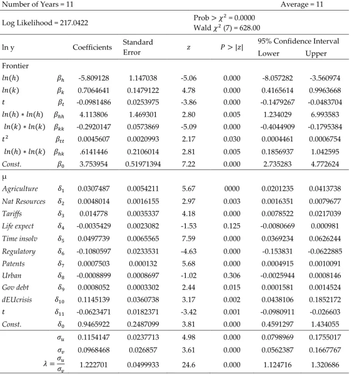
4.1. Empirical model specification and estimates ... 47
4.2. Inefficiency ... 50
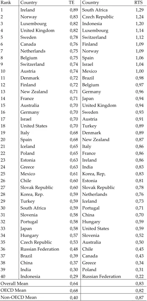
4.3. Technical efficiency and returns to scale ... 58
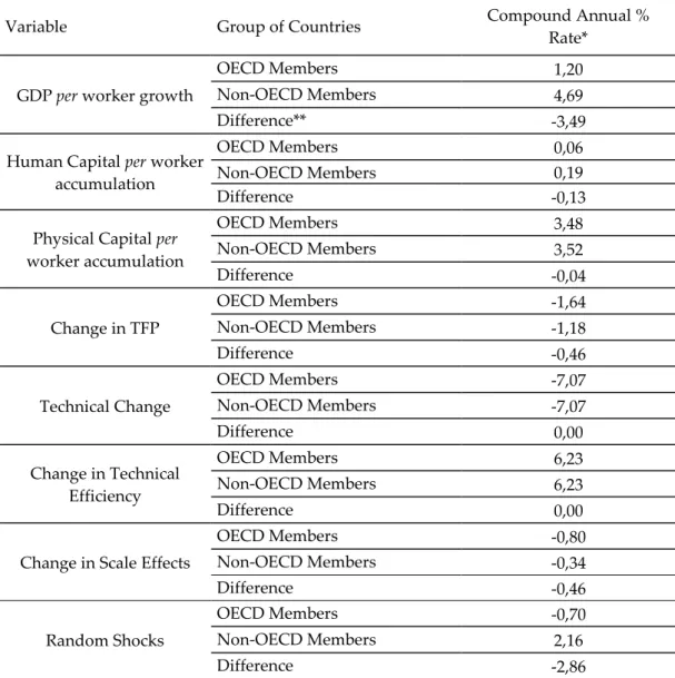
4.4. Decomposition of economic growth ... 61
5. Conclusion ... 64
Bibliography ... 66
List of Figures
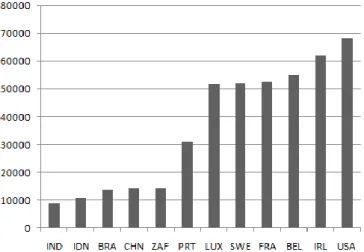
Figure 1: GDP per person employed (constant 1990 PPP $) in 2011 ... 1
Figure 2: Production Frontiers obtained from CRS-DEA and VRS-DEA ... 16
Figure 3: Stochastic Production Frontier ... 19
Figure A.1: Productivity, Technical Efficiency and Scale Economies ... 77
Figure A.2: An input-oriented measure of technical efficiency (N=2) ... 79
Figure A.3: An output-oriented measure of technical efficiency (M=2,N=1) ... 80
List of Tables
Table 1: Methodologies used to measure productivity ... 8 Table 2: Comparison in levels of OECD and emergent countries for 2011 ... 42 Table 3: Comparison in growth rates of OECD and emergent countries for 2011 ... 42 Table 4: Stochastic Frontier Time-Varying Inefficiency Model ... 49 Table 5: Rankings in levels: Technical Efficiencies and Returns to Scale ... 61 Table 6: Sources of economic growth 2001–2011 per groups of countries:
1. Introduction
Presently, it is widely accepted that differences in efficiency and productivity growth greatly contribute to the enormous differences in income across countries. Therefore, the purpose of this research is to evaluate the efficiency and productivity growth of nations and explore the causes behind those differences. Inefficiency levels will be estimated using a stochastic frontier model based on the Battese and Coelli (1995) time-varying inefficiency model and productivity growth will be decomposed using the Kumbhakar and Lovell (2000) primal frontier approach.
Jones and Romer (2010) selected the large differences in income across countries as one of the new stylized factors. According to the World Bank’s World Development Indicators, in 2011, USA’s output per worker (converted to 1990 constant international dollars using PPP rates) was approximately 7.5 times higher than output per worker in India. Intuitively, this means that a worker in America produces in one hour approximately as much output as a worker in India produces in an entire day.
Figure 1: GDP per person employed (constant 1990 PPP $) in 2011
But why are some countries far richer than others? Determining the causes of the discrepancies in the levels of production, and consequently in the standards of living, across countries, is a demanding and complex challenge that several authors have tried to address.
In order to understand the enormous disparities in economic performances between countries, one should consider first looking at the determinants of economic growth, that is, factors that explain the increase in a country’s income per capita over a long period of time. One of the most famous attempts to explain those determinants was presented by Solow (1956, 1957), which established the roots of the neoclassic theory of economic growth. In his 1956’s seminal article, Solow delivered his neoclassical model, which can be seen as an extension of the Harrod-Domar model. He demonstrated that, in order to sustain long-term economic growth, there must be continuous advances in technology so to contradict the effects of diminishing returns that would in due course cause economic growth to cease. The 1957 article established the accounting framework for explaining income growth. By assuming a Cobb-Douglas production function, Solow was able to decompose economic growth into contributions from factor accumulation (such as labor and capital) and total factor productivity (henceforth TFP). He found out that the growth rate of productivity, measured as a residual term, the Solow residual, has a predominant role in determining the GDP per capita growth rate.1 Following the
same line of thought, Kuznets (1971) concluded that the high rate of productivity growth accounts for most of the growth of product per capita. He reported that, even considering hidden costs and inputs, growth in productivity accounts for more than half of the growth in output per capita. Consequently, if the rate of change of productivity exerts such enormous influence on the growth rate of GDP per capita, as advocated by these two authors, according to
1 Recall that the growth rate of TFP is given by: ̂( ) ( ) ( ) ( ) ( ) ( ), where
the Solow model, it can be concluded that most of the economic growth is exogenously determined. Therefore, reliance on the exogenous technological progress as an essential variable to explain economic growth poses one of the biggest limitations of the initial neoclassical approach. This point of view was first expressed by Moses Abramovitz, who dubbed this term “a measure of our ignorance about the causes of economic growth” (Abramovitz, 1956).
Latter attempts to scrutinize the content of the Solow residual gave rise to a new set of theories named “endogenous growth theories”. By endogenizing a country’s technology, these theories advocate that factor accumulation is not sufficient to explain differences in income growth and try to explain the differences in the growth of the residual by analyzing the choices of the public and private sector.2 As an example, in Romer’s (1990) model, growth is
motivated by technological change that emerges from deliberate investment decisions made by profit-maximizing agents. According to its defenders, these theories provide policymakers with more relevant information regarding the determinants of long-run economic growth than the standard neoclassical framework.
However, in the recent past there have been a plethora of empirical studies that contradicted the idea that physical and human capital accumulation did not suffice to explain the differences in levels and growth rates of output. Mankiw, Romer and Weil (1992) concluded that the augmented Solow model (an extension of the original neoclassical Solow model that includes human as well as physical capital) provides a very good picture of the cross-country data. They predicted that the augmented Solow model accounts for about 80% of the cross-country variance in income in 1985. Alwyn Young (1994) documented the fundamental role played by factor accumulation (rather than the rise in
2 The neoclassical framework postulated that a common (exogenously determined) technology was shared
by every country due to the non-rivalry and non-exclusivity nature of the technological progress (note that the growth of the residual, that is the growth of productivity, essentially mirrors this technological progress). Consequently, technological progress could not explain differences in GDP per capita across countries and one had to look for differences in the factor accumulation.
productivity) in explaining the astonishing post-war growth of the East Asian countries. Klenow and Rodriguez-Clare (1997) called these set of studies the “neoclassical revival”, mainly because they advocate that differences in physical and human capital are the main contributors to the differences in the level and growth rate of GDP.
The lively debate that one has witnessed is based on the relative importance of factor accumulation or productivity in contributing for differences in economic performance. Simply put, ( ), where factors include physical and human capital, and economists do not seem to agree on which variable (factors or productivity) contributes more to the differences in income levels and growth rates. According to Klenow and Rodriguez-Clare (1997), this debate is of great importance because the implications of each view (the factors or the productivity view) can differ substantially. For instance, technology-based models of productivity, by assuming scale effects due to the non-rival nature of technology creation and adoption, propose that international trade openness can have direct effects on income levels and growth rates. The neoclassical approach does not share this view, and assumes that productivity is common across countries. More recently, this crucial assumption was again questioned by several empirical studies – Knight, Loyaza and Villanueva (1993), Islam (1995) and Caselli, Esquivel and Lefort (1996), to name a few – which proved that the income-convergence predicted by the neoclassical framework is occurring but conditionally to the existence of differences in productivity between countries. In fact, by analyzing recent contributions to the economic growth literature, one can observe an increasing focus on the productivity growth as the main driver of long-term income growth and cross-country differences in income. Klenow and Rodriguez-Clare (1997) used the Mincer-regression to estimate the levels and growth rates of human capital, found out that differences in the level and
income levels and growth rate. Hall and Jones (1999) focused on levels instead of growth rates and calculated the TFP level as the Solow residual. They concluded that differences in physical and human capital can only partially explain differences in GDP per worker and that a great part of the variance in income per capita is due to a large fluctuation in the level of the Solow residual across countries. Easterly and Levine (2001) identified the TFP as the main contributor to the cross-country differences in the level and growth rate of income per capita and named it a stylized factor. In 2013, the Organization for Economic Co-operation and Development identified the productivity growth as a key factor to improve income per capita and hence standards of living.
The results in recent economic growth literature, by favoring the importance of productivity over factor accumulation in explaining the differences in income levels and growth, gave rise to the need of better comprehend TFP and its determinants in order to design policies most conducive to TFP growth, and consequently, long-run economic growth. Consequently, several authors have tried to address this issue. These studies emphasize the importance of institutions and government policies (Hall and Jones, 1999; Acemoglu et al., 2004; Afonso and St. Aubyn, 2013), human capital (Barro, 2001; Aiyar and Feyrer, 2002; Afonso and St. Aubyn, 2013), trade openness (Edwards, 1998; Baldwin and Gu, 2003; Dollar and Kraay, 2004), the roles of natural resources (Delíktas and Bacilar, 2005), among others, in boosting productivity growth.
By estimating the total factor productivity change (TFPC) for the 34-OECD countries plus the emergent economies of Brazil, China, India, Indonesia, Russian Federation and South Africa for the 2001-2011 period and evaluating the relative contribution of each factor to their efficiency, and consequently to their TFPC, this empirical study intends to be a valuable contribution to the ongoing debate on the determinants that foster productivity growth.
This work proceeds as follows: chapter 2 provides a literature review of the existing methods to estimate efficiency and productivity changes. Chapter 3
provides a brief description of the the Battese and Coelli (1995) time-varying inefficiency model as well as a description of the data and the estimated model. Chapter 4 provides the results and their discussion. Lastly, chapter 5 states the concluding remarks.
2. Literature Review
The ability of a nation to convert inputs, such as human and physical capital, into outputs, influences its capacity to generate long-run economic growth, and consequently, to improve the standards of living of its society. This ability, commonly referred to as productivity, can be analyzed for a number of other decision making units (DMU’s) such as firms, plants, industries or regions, and its measurement has been made in different research fields.3
The general idea behind the calculation of productivity is based on the fact that it reflects output differences that cannot be explained by differences in the factor accumulation. To put it formally, one can think of a production function of the type
( ) ( )
where Y, the output of a decision making unit (firm/plant/industry/region/country) i in period t, results from the combination of (1 x N) vector of inputs X and the term A, which reflects the amount a given DMU is capable of producing from a certain quantity of inputs, given the technological level.4 Hence, is the TFP for the DMU i in period t and can be
calculated as the ratio of produced output to total inputs used:
( ) ( )
3When productivity is mentioned, one is referring to the total factor productivity, also known as
multifactor productivity, although there are several other measures of productivity. See Measuring Productivity OECD Manual (2001) for a brief sum up of the main productivity measures.
4
Note that F(.) reflects the state of technology and is assumed to be common to all DMUs. This assumption prevails in the traditional neoclassical framework, where (index i dropped) represents
simultaneously productivity growth and technological progress. Further in the analysis, one will drop the assumption of common technology among units, which will dismantle the equality between productivity growth and technological progress, and one will decompose TFP growth into its several sources.
A wide range of methodologies for productivity estimation is available, and researchers have to choose the one that best suits their purposes. To facilitate this process, Del Gatto et al. (2011) proposed a way of grouping the different methods of productivity measurement, which one will follow. Although this approach does not consider all the existing methods, it comprises the main blocks of techniques for productivity estimation. They use three main criteria: (i) whether the method allows for a micro and/or macro analysis; (ii) whether it is a frontier or a non-frontier approach and (iii) whether it is a deterministic or econometric method. Deterministic Methodologies Econometric Methodologies Parametric Semi-Parametric Frontier
Data Envelopment Analysis (DEA)
(Micro/Macro)
Free Disposal Hull (FDH)
(Micro/Macro) Stochastic Frontier Analysis (SFA) (Micro/Macro) Non-Frontier Growth Accounting (Macro) Index Numbers (Micro/Macro) Growth Regressions (Macro) Proxy-Variables (Micro)
Table 1: Methodologies used to measure productivity
Source: Del Gatto et al. (2011), Measuring Productivity
Del Gatto et al. (2011) start their analysis by dividing methodologies according to the type of data sets that they can be applied to. Methods applied to macro data sets measure productivity of aggregate units (industries, countries, regions), while techniques that use micro data sets aim to measure productivity of individual units (firms, plants). As Table 1 shows, this criteria is not mutually exclusive, as there are methods that can use both micro and macro data (DEA, FDH, SFA and Index Numbers). Then, the authors distinguish
between frontier and non-frontier models. Frontier models allow for the existence of inefficiency in the productive processes, while non-frontier models assume that the observed output always equals the potential level of production at each moment in time.5 Finally, they divide the surveyed methods
between deterministic, where the measure of TFP is calculated, and econometric, where TFP is estimated.
An extensive comparison between non-frontier and frontier models goes beyond the scope of this analysis, which is to provide sufficient background to understand the frontier method used to calculate inefficiency and decompose TFP presented in the next chapters. Consequently, only a brief review on the non-frontier models will be presented and a more detailed discussion is provided in the Del Gatto et al. (2011) survey.
2.1 Non-Frontier Models
Non-frontier methodologies comprise methods that can be applied to (i) aggregate data sets only, such as the growth accounting and the growth regressions methods; (ii) individual data sets only, such as the proxy-variables models; (iii) both aggregate and individual data sets, such as the index numbers method.
The first attempts to measure productivity growth were performed using aggregate data of the US economy, via growth accounting methodology (Abramovitz, 1956; Solow, 1957). Under this method, TFP growth (also known as Solow residual or technological progress) was calculated as the difference between output growth and a weighted average of the inputs growth rates. The authors found out that the TFP growth was responsible for almost 90% of the
5 This assumption results from the fact that the latter methods assume that units share the same
output growth. Several extensions of this methodology were proposed in order to overcome some limitations in the estimation of the residual. In particular, the level accounting methodology, although it shares the same objective of the previous methodology, it estimates TFP levels instead of growth rates. Hall and Jones (1999) support this extension, advocating that recent contributions to the economic growth literature focus in levels instead of growth rates and prove that cross-country differences in growth rates are merely transitory (Easterly et al., 1993; Parente and Prescott, 1994; Barro and Sala-i-Martin, 1995).
Growth regressions are an alternative methodology to estimate TFP. Although it is also an extension of the original Solow model, this approach has the advantage of estimating TFP from a structural equation that it identifies and not from a residual exercise. Furthermore, it has the advantage of not requiring the use of data on physical capital stocks, as it is very likely to contain significant measurement error problems.
More recently, studies started to focus on estimating firm-level productivity, essentially due to the development of a theoretical literature based on the assumption of heterogeneity among firms and the increasing availability of individual data. The proxy-variable method was developed to mitigate the problems related to estimating firm-level productivity, such as simultaneity, price dispersion and selectivity. It consists of identifying a proxy variable that is a function of the TFP (such as intermediate goods or investment) and calculating the inverse of that function, in order to express TFP as a function of the proxy variable itself.
Index numbers, the last non-frontier model mentioned in the survey, can be applied to both micro and macro data sets. Index numbers can be used to calculate changes in TFP directly from input and output prices and quantities, known as the TFP index numbers. The indexes most widely used to measure
productivity are the Törnqvist, the Laspeyres, the Paasche and the Fisher. Notice that index numbers can also be used together with frontier models (the Malmquist productivity index).
One characteristic that is common to all previously mentioned methods is the fact that they expect producers (either in aggregate or in individual terms) to be fully efficient, meaning that they operate on the production frontier, where observed output matches potential output. Yet, in the presence of inefficiency, both productivity measurement and productivity change will be affected, assuming that inefficiency varies over time. Consequently, measurements of TFP growth based on non-frontier methods will lead to biased results. Frontier models account for the presence of inefficiency and their main advantage over the non-frontier models is their capability of decomposing two main sources of productivity growth: technical efficiency change and technical (or technological) change. This characteristic provides useful information to the policymakers, since policies required to address these two sources of productivity growth are likely to be different. For instance, technological progress can be promoted using policies that induce innovation (such as public investment in R&D), while efficiency requires, for instance, policies oriented to education improvement. Frontier models will be presented in the following subchapter.
2.2 Frontier Models
Frontier models presuppose the existence of physical or economic representations of the production technology. Economic representations of the production technology include cost, revenue and profit frontiers and, contrarily to the production frontier, they require the use of information on both prices and quantities of inputs and outputs and an imposition of a behavioral
objective on producers. These frontiers result from the optimization problem that the producer successfully solves – at least in theory. In the case of a production frontier, it represents the maximum attainable output from a set of inputs, given the technology available, or alternatively, the minimum amount of inputs necessary to produce a given level of output, at the current technology level. The cost frontier gives the set of inputs that minimize the cost of producing a given level of output with the available technology and given the input prices, while the revenue frontier shows the set of outputs that maximize revenue from a given set of inputs, given the output prices and the available technology. The profit frontier results from the maximization of revenue and minimization of cost. While a production frontier represents the best set of inputs or outputs that can be achieved technically, the last three frontiers represent the best combinations that can be achieved in economic terms.
There is, however, empirical evidence that shows that producers do not always successfully solve their optimization problems. In fact, those frontiers are used as benchmarks to make relative economic performance evaluations, where distances to a particular frontier provide measures of efficiency. Technical efficiency is measured as the distance to a production frontier, while allocative efficiency is represented by the distance to an economic (cost, revenue or profit) frontier. The combination of both efficiencies constitutes the “overall efficiency” concept.6
The recognition that inefficiency exists and that it affects productivity led to the creation of methods capable of incorporating it into the measurement of the latter: the frontier methods. This characteristic and their capability of decomposing the sources of productivity change made them a very popular
6 One will forego the concepts of allocative and overall efficiency as well as economic frontiers in the
overview of technical efficiency and productivity change-related concepts presented in Appendix A, since the empirical analysis performed in chapter 3 will not consider the prices of inputs or outputs. This brief overview intends to be a helpful insight in understanding the mechanisms behind the frontier model used
instrument used in several empirical studies of TFP growth. TFP growth will now explicitly result from a decomposition of productivity change into technological change, which pushes the frontier of feasible production upward, and efficiency change, which corresponds to movements towards the production frontier. The Del Gatto et al. (2011) survey named three frontier methods that can be applied to both micro and macro data sets: data envelopment analysis (DEA), free disposal hull (FDH) and stochastic frontier analysis (SFA).
According to Del Gatto et al. (2011), one can distinguish FDH and DEA from SFA using the deterministic/econometric criteria: while in DEA and FDH, the estimation of frontier functions and the measurement of technical efficiency are performed in a deterministic environment, the latter assumes a stochastic context. Thus, while the first two methods involve mathematical programming, the last one requires econometric methods. It is the nature of these methods that provide their main advantages and limitations. On the one hand, the first set of methods, because of their deterministic nature, assumes that all deviations of observed output from potential output are due to technical inefficiency. Consequently, all observations lie on or below the production frontier. Any other possible source of these deviations, i.e. unobserved measurement errors, omitted variables and stochastic noise, is not considered, which may result in an upward bias of inefficiency measures. Additionally, DEA and FDH require large data sets in order to better approximate the “best-practice” frontier to the real production frontier. Although traditional literature on DEA presented, as a limitation of this methodology, the fact that it did not allow for the estimation of standard errors and tests of hypothesis, recent literature has shown that it is possible to define a statistical model that allows for the determination of statistical properties of the non-parametric frontier estimators (Simar and Wilson, 2000).
On the other hand, the deterministic frontier approaches do not require the imposition of a functional form for the technology set. The stochastic frontier approach, by separating the error term into an inefficiency term and a noise term, allows the distinction between inefficiency and other causes of the differences between the observed output and the potential one. This separation is only possible due to the imposition of a distributional form for the inefficiency term, which might affect the results considerably. Likewise, the imposition of a specific functional form for the production frontier constitutes another important limitation.
Empirical works have used extensively both DEA and SFA, but not the FDH model, created by Deprins et al. (1984). Although it constitutes a more flexible model than the DEA (as it only assumes free disposability while DEA assumes also convexity) the FDH model did not gain much acceptance among the efficiency measurement studies. For this reason, one will not consider this model in the following analysis of the most widely used frontier models.7
2.2.1 Data Envelopment Analysis (DEA)
The idea behind the DEA approach to measure TFP change consists in using linear programming methods to envelope the observed combinations of input and outputs in order to construct a non-parametric piecewise surface (also known as the “best-practice” frontier) so that all observed points lie on or below that frontier and then use it to identify the contribution of the different sources of the TFP change.8
7
The following analysis was adapted from Coelli (1995).
8
For the purpose of this analysis, in the DEA framework, one will consider the estimation of technical efficiency but not the estimation and decomposition of productivity change. The estimation and decomposition of productivity change will be mentioned for the SFA framework, as it is the framework used in the empirical analysis performed in chapter 3, and TFP change will be estimated and decomposed
The piecewise-linear convex hull method to estimate frontiers proposed by Farrell (1957) did not receive much attention until Charnes, Cooper and Rhodes (1978) changed it into a mathematical programming problem, which they called data envelopment analysis (DEA). They proposed an input-oriented model with constant returns to scale (CRS). Subsequent papers presented extensions of the original model by assuming different assumptions, such as Banker, Charnes and Cooper (1984), who presented the variable returns to scale (VRS) model.
The Constant Returns to Scale (CRS) Model
Let’s assume there is information regarding K inputs and M outputs for each of the N firms. The KxN input matrix, X, and the MxN output matrix, Y, represent the data for all the firms. One way of representing the CRS model is through the definition of a linear programming problem:
st.
( )
where is a Nx1 vector of constants and is a scalar, representing the efficiency score for the i-th firm. varies between 0 and 1, where 1 indicates a point in the frontier meaning that the firm is technically efficient. This linear programming problem has to be solved N times because is obtained for each firm.
The Variable Returns to Scale (VRS) Model
The constant returns to scale assumption works well in a perfectly competitive scenario, where all firms operate at the optimal scale. However, imperfect competition, government regulations, constraints on finances,
externalities, among others, may cause firms to not operate in the optimal scale. In these cases, technical efficiency measured under the CRS framework is biased by scale efficiencies. An extension of the CRS was proposed by Banker, Charnes and Cooper (1984) to correct this shortcoming: the variable returns to scale (VRS) model. The VRS linear programming problem can be derived from the previous CRS programming problem by adding the convexity constraint, : st ( )
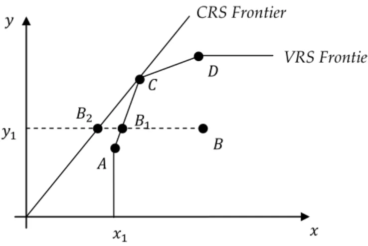
where N1 is an unitary vector (Nx1). This approach provides a “tighter” frontier to the data points and thus the technical inefficiency scores that result from it are less than or equal to the ones obtained from the CRS model. Another advantage of this model over the CRS model is the fact that it ensures that an inefficient firm is compared with firms of a similar size. Figure 2 shows the differences between the frontiers obtained from a CRS model and a VRS model for the case of one input and one output. One can see the implications of each method on the input-efficiency measures. For the case of firm B, using the CRS-DEA model, its technical inefficiency is given by the distance , while in the case of the VRS-DEA model, the technical inefficiency is given by the distance , where ̅̅̅̅̅ ̅̅̅̅̅.
Figure 2: Production Frontiers obtained from CRS-DEA and VRS-DEA
Output-Oriented Models
The previous input-oriented models aimed to identify technical inefficiency as a proportional drop in the input quantity, holding output levels constant. This is the Farrell’s input-oriented measure of technical inefficiency. It is also possible to compute technical inefficiency as a proportional increase in output production, holding input levels constant. The two measures of inefficiency provide the same results under the CRS assumption, but not under VRS. The choice of the orientation of the model will depend on the purpose of each firm: either to maximize output maintaining the input levels fixed or to minimize input usage for the current output level (for example, when a firm has orders to fill and thus the input quantities seem to matter the most). These models are very similar to their input-oriented counterparts. In particular, the output-oriented CRS model can be defined from the following linear programming problem: st ( ) CRS Frontier VRS Frontier
where corresponds to the proportional increase in outputs that the i-th firm can achieve. To obtain the output-oriented VRS model, just add convexity constraint, .
One last note on the input and output-oriented models regards the fact that both estimate the same frontier and consequently the efficient firms are the same. It is only the efficiency measures of the inefficient firms that may change.
Other Extensions
Recent developments in the DEA approach include: the measurement of allocative efficiency assuming availability of price information and a behavioral objective such as cost minimization (Ferrier and Lovell, 1990), revenue maximization (Färe, Grosskopf and Lovell, 1985) or profit maximization (Färe and Grosskopf, 1997); non-discretionary variables (Banker and Morey, 1986; Afonso and St. Aubyn, 2013); environmental variables (Fried, Schmidt and Yaisawarng, 1999); incorporation of a stochastic element (Sengupta, 1990); panel data and Malmquist index approach to calculate technical change and technical efficiency change (Färe et al., 1994).
2.2.2 Stochastic Frontier Analysis (SFA)
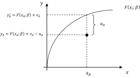
The stochastic frontier analysis was pioneered by Aigner, Lovell and Schmidt (1977) and Meeusen and van den Broeck (1977). These authors, independently, proposed the estimation of the following stochastic frontier:
( ) ( ) ( )
where is the output produced by firm i, is the vector of input quantities used by firm i, ( ) represents the production function, a vector of unknown
parameters to be estimated, is the symmetric noise component of the error term assumed to be independently and identically distributed as ( ) and is the non-negative technical inefficiency component of the error term, independent of and derived from a ( ) distribution truncated above at zero.9 The firm’s observed level of production is bounded above by the sum of a
parametric function of known inputs (and unknown parameters) and a random error term reflecting measurement error of the level of production or other external factors, such as climate, strikes, economic crisis that cause the position of the deterministic part of the frontier, ( ), to vary across firms. The greater the difference between realized production, ( ) , and the corresponding stochastic frontier level of production, ( ) , the greater the level of technical inefficiency.
Figure 3: Stochastic Production Frontier
The output-oriented measure of technical efficiency is then given by the ratio of observed output to the corresponding stochastic frontier output:10
9 Note that when , this model becomes a deterministic frontier model.
10According to Aigner, Lovell and Schmidt (1977), this is the correct measure of technical efficiency,
instead of ( ( )), because the first ratio distinguishes technical inefficiency from other sources of disturbance that the firm cannot control.
( )
( )
( ( ) ) ( ( ) ) ( ( ) ) ( ( )) ( ) ( ) ( ( )) ( ) ( ) ( )
The technical efficiency measure, , varies between 0 and 1. In order to estimate it, one has to estimate first the parameters of the stochastic production frontier. The β’s in this model are estimated using the Maximum Likelihood (ML) method, under the assumption that the error terms follow appropriate distributions. In particular, Aigner, Lovell and Schmidt (1977) assumed that is independently and identically distributed following a normal distribution and that is distributed independently of and derived from a half-normal or an exponential distribution. The other possible method to estimate the parameters is the COLS method. Although the COLS method is computationally less demanding than the ML method, the latter is asymptotically more efficient, making it a more popular estimation method.
This stochastic model allows the overcoming of two of the limitations of the traditional deterministic models: no consideration of noise and the impossibility of estimation standard errors and tests of hypothesis. However, this model has some other limitations, as mentioned before. In particular, the selection of a specific distributional form for the inefficiency term without a solid a priori justification constitutes an important limitation, which can be partially solved with the assumption of more general distributions, such as the truncated-normal or the two-parameter gamma. Another important limitation of this model is the imposition of a specific functional form for the production frontier. The most common production function used in empirical estimations of frontier models is the logarithmic transformation of the Cobb-Douglas, mostly due to its simplicity. However, this form imposes strong restrictions: returns to scale are equal for all firms and elasticities of substitution are equal to one. One way of
more flexible ones. In particular, the translog form, although it is not flawless, imposes no restrictions on the returns to scale and the elasticities of substitution.
Panel Data
Up to this moment, the estimation of the frontier was performed in the cross-sectional framework, i.e., the case of N firms observed at one moment in time. The case of multiple firms observed in several moments in time, i.e., the panel data case, provides a richer set of information, which is proved to have many advantages for the frontier estimation. In particular, panel data provides consistent estimators of firm efficiencies (given that T is large); increases the degrees of freedom; eliminates the need to make assumptions on the distribution of the ; does not require independency between the inefficiencies and the regressors and allows for the estimation of both technical change and technical efficiency change over time.11 Islam (1995) states that the main
advantage of the panel techniques is related to the fact that it allows for differences in the aggregate production function across countries. Temple (1999) argues that the panel data approach allows to control omitted variables that are persistent over time, which otherwise could cause estimation problems.
Pitt and Lee (1981) presented an extension of the Aigner, Lovell and Schmidt (1977) half-normal model to account for panel data:
( ) ( ) ( )
which parameters were estimated using ML estimation. This model accommodates the situation where technical inefficiency varies across
11 The importance of not requiring the inefficiencies to be independent of regressors can be seen, for
producers and over time for each producer. The authors also proposed a model where technical inefficiency varies across producers but is constant over time:
( ) ( ) ( )
Battese and Coelli (1988) provided an extension of this model that allowed the to have a truncated normal distribution. These models provide consistent estimators of the when T is large. However, the assumption of time-invariant technical inefficiency is reasonable only when the time period is short, since managers are expected to improve their performance based on previous experience.
Kumbhakar (1990) and Battese and Coelli (1992) proposed extensions of the Pitt and Lee (1981) time-varying inefficiency model that take the form:
( ) ( )
where ( ) is a function that determines the way technical inefficiency varies over time. For the Kumbhakar (1990) model, ( ) ( ) and has an half-normal distribution, while for the Battese and Coelli (1992) model, ( ) ( ) and is assumed to have truncated normal distribution. , and are parameters to estimate. The inclusion of the time trend allows for the estimation of both technical change and technical inefficiency change over time. Cornwell et al. (1990) proposed an alternative specification of the time-varying inefficiency term: . Lee and Schmidt (1993)
assumed , where are time dummies representing the time effects
and are either fixed or random firm-specific effects.
The previous presentation did not involve a comprehensive review of the panel data stochastic frontier models. A list of other panel data stochastic frontier models is provided in Appendix B.
Determinants of Inefficiency
The ability of a firm to convert inputs into outputs is influenced by the exogenous variables that characterize the environment in which the production takes place. These variables are neither the inputs nor the outputs of the production process, but nonetheless affect the performance of the firm.12
Empirical studies that have explored the relationship between environmental variables and estimated technical efficiencies include Pitt and Lee (1981), Kalirajan (1981, 1989) and Kalirajan and Shand (1989). These papers adopt a two-stage approach, in which the first-stage estimates either the inefficiency effects or the technical efficiencies of the firms using an estimated stochastic frontier (excluding the exogenous variables) and the second-stage involves regressing them on the environmental variables. Through the second-stage, one can see that exogenous variables influence the output indirectly, through its effect on predicted inefficiency effects or the levels of technical efficiency. Exogenous variables do not influence the production frontier, but they influence the position of the producer in relation to the frontier. This approach has, however, some econometric problems. In the first place, it is assumed in the first-stage that the inefficiencies are identically distributed, yet this assumption is contradicted in the second-stage, where they are assumed to have a functional relationship with the exogenous variables. Secondly, the exclusion of the environmental variables in the first-stage leads to biased estimators of the parameters of the production frontier and biased technical inefficiency measures, in the case where exogenous variables are correlated with the regressors.13
To overcome these inconsistencies, Pitt and Lee (1981) investigated the sources of technical inefficiency by regressing the estimated firm intercepts on
12 One will consider only non-stochastic variables, which are the ones that are observable at the time
production decisions are taken (eg. degree of government regulation, age of the labor force). Stochastic variables can be interpreted as sources of production risk (eg. weather).
firm specific characteristics or by including these variables into the production frontier and jointly estimate the parameters. More recently, Kumbhakar, Ghosh and McGuckin (1991), Reifschneider and Stevenson (1991) and Huang and Liu (1994) proposed stochastic frontier models in which inefficiencies are an explicit function of the firm specific factors and the parameters are estimated using a single-stage ML estimation. Kumbhakar, Ghosh and McGuckin (1991) assumed technical inefficiency effects as non-negative truncations of a normal distribution with the mean being a linear function of exogenous variables with unknown coefficients, and unknown variance. The authors considered also the allocative inefficiency effects which result from the failed attempt to profit maximization. In the empirical application of their model, the authors found out that the farmers’ level of education and the size of their farming operations affect technical inefficiency significantly. Reifschneider and Stevenson (1991) presented a model where the technical inefficiency effects are a function of non-negative explanatory variables and a non-non-negative random variable, which has a half-normal, gamma or exponential distribution. The model was applied to the generation of electricity in the USA in three separate periods. They concluded that the inefficiency function is important to the estimation of the production frontier. Huang and Liu (1994) proposed a model where the non-negative technical inefficiency effects are a linear function of variables that reflect firm characteristics and a random error term, which is the truncation of a normal distribution with zero mean and whose point of truncation depends on the firm characteristics. The authors investigated the electronics industry in Taiwan in a cross-section framework. Battese and Coelli (1995) proposed an extension of the Huang and Liu (1992) model to account for panel data, where the technical inefficiencies are a function of firm-specific variables and time.14
The inclusion of the time variable allows for the estimation of technical efficiency change and technical change. The model was applied to paddy
farmers in Aurepalle, India, for the period 1975-1985 and the authors found out that the farmers’ age increases inefficiency and schooling has the opposite effect.
Decomposition of TFP Change
So far, the discussion has focused on estimating technical inefficiencies from cross-sectional or panel data. In the presence of panel data, we can move one step further and estimate TFP change and decompose it into its various sources. This raises two questions: (i) how can productivity change be measured; and (ii) what are the sources of productivity change. Diewert (1992) provided an answer to question (i): given that productivity change occurs when an index of outputs and an index of inputs change at different rates, he proposed the use of index number techniques to construct a Fisher or Törqvist productivity index. However, these indexes require price and quantity information, as well as assumptions on the structure of technology and on producers’ behavior. Productivity change can also be estimated using non-parametric techniques (such as DEA) or econometric approaches (such as SFA) to construct a Malmquist productivity index. This index does not require price information or assumptions on producers’ behavior, although it still requires information on the structure of technology.
Although both types of techniques (index numbers and parametric/econometric techniques) provide answers to question (i), only non-parametric/econometric techniques provide an answer to question (ii) and only econometric techniques do it in a stochastic environment.
A stochastic frontier approach to the estimation and decomposition of the TFP change in a panel context is proposed by Kumbhakar and Lovell (2000). The primal (production frontier) approach, as the authors named it, consists in
a quantity-based method in which they propose the use of econometric techniques to estimate a production frontier against which the magnitude of productivity change is estimated and then decomposed into its various sources, namely a technical change component, a returns to scale component and a technical efficiency change component.
The general stochastic production frontier model is presented in equation ( ), where is the vector of output produced, ( ) is the deterministic part of the stochastic production frontier, is the vector of production factors used, is the vector of the parameters defining the production technology, t is the time trend serving as a proxy for technical change, ( ) is the random error term and ( ) is the output-oriented technical inefficiency.
( ) ( ) ( ) ( )
Given the previous assumptions on the distributions and independence of the two error components, and , the model can be estimated by ML. Once maximum likelihood estimates of the parameters in ( ) are obtained, we can decompose TFP change for each producer into its various sources.
A measure of the rate of technical change is given by:
( )
( )
where means an upward shift in the production frontier and technological progress, represents a downward shift in the production frontier and technological regress and means that the frontier remained unchanged. Technical efficiency change can be given by:
where means that the producer moved towards the production frontier, that is, became more efficient, represents a movement away of the frontier and means that the position of the producer in relation to the production frontier remained unchanged. For the scalar output case, TFP change is defined by a Divisia index of productivity change:
̇ ̇ ̇ ̇ ∑ ̇ ( ) where a dot over a variable represents its rate of change, is the observed expenditure share of the input , ( ) is an input price vector and ∑ is the total expenditure. In the absence of price information, , where ( ) are the elasticities of output with respect to each of the inputs and ∑ is the scale elasticity, which provides a measure of returns to scale characterizing the production frontier.
̇ ̇ ∑ ( ) ̇ ( ) By differentiating the deterministic part of ( ), we obtain:
̇ ( )
∑ ̇
( )
Combining ( ) and ( ), we have:
̇ ( ) ∑ ̇ ∑ ( ) ̇ ( ) ( ) ∑ ̇ ( ) ( ) ∑ ( ) ̇ ( ) ∑ ( ) ̇ ( )
Equation ( ) exhibits the decomposition of the productivity change into a technical change component ( ), a scale component [( ) ∑ ̇ ] and a technical efficiency component ( ). If either production technology or technical efficiency does not change through time, it does not affect productivity change. The influence of scale economies on productivity change depends on the type of technology and the input usage. Assuming constant returns to scale, the change in the input usage will not alter productivity change. However, under non-constant returns to scale, input growth (∑ ̇ ) and scale elasticity or input contraction (∑ ̇ ) and scale elasticity lead to an increase in total factor productivity.
So far, we have decomposed TFP change from the general stochastic production frontier model in equation ( ). To provide a good basis for the TFP change estimation and decomposition performed in chapter 3, one will consider the panel data case of I producers through T periods of time and a time-varying production frontier expressed in the following translog form:
∑ ∑ ∑
∑ ( )
where ( ) is random error term and is the technical
efficiency error term. Additionally, we consider the technical inefficiency function suggested by Battese and Coelli (1995), although there are several other possible parameterizations of the 15,16:
( ) ( )
15 We present some alternative parameterizations of the previously in the present subchapter.
16 Although the original parameterization of the technical inefficiency is , we decided to add
explicitly the time variable – as the authors did in their empirical application – in order to show how the decomposition of TFP change is performed.
where ’s are non-negative truncations of the (( ) )-distribution
and is the random variable defined by the truncation of the normal
distribution with zero mean and variance .
One can see that the time variable shows up in the production frontier and in the second error term. According to Kumbhakar and Lovell (2000), the main econometric problem is to separate the two roles played by : as a proxy for the technical change in the deterministic part of the stochastic production frontier and as an indicator of technical efficiency change in the second error term, . In specification ( ) the separate time effects can be disentangled by linearly adding the variable . Based on the previous assumptions regarding the distributions and independence of and , the probability density function
of the composite error term, , is derived and the log likelihood function
for the model ( ) is obtained. By maximizing the log likelihood function, one obtains estimates of the parameters of the model, which one can then use to predict technical inefficiencies. From equation ( ), we can see that the estimation and decomposition of TFP change require the estimation of and , which can be obtained after the estimation of the parameters of the model: ̂ ( ̂) ̂ ̂ ∑ ̂ ( ) ̂ ̂ ̂ ( ) ̂ ( ̂) ̂ ∑ ̂ ̂ ( ) ̂ ∑ ( ̂ ∑ ̂ ̂ ) ( )
TFP change can be obtained for each producer by substituting ( ) ( ) into ( ). Notice that, if no restrictions are made, all components of equation ( ) are time specific and all components except are producer specific. varies across time, unless , and across producers, except if
technological progress is neutral with respect to the inputs ( ).
varies across time, following the same path across producers, unless . ( ) ∑ ( ) ̇ varies across time and producers except when technology
is of the Cobb-Douglas type (∑ and ) or ̇
. We will test these parametric restrictions in chapter 3.
2.2.3 Empirical Applications of Frontier Models to Evaluate the
Efficiency Productivity Growth of Nations
The frontier models presented in the previous discussion considered firms in a particular industry as the unit of analysis (Pitt and Lee, 1981; Kalirajan, 1981, 1982, 1989; Kalirajan and Flinn, 1983; Kalirajan and Shand, 1989; Kumbhakar, 1991; Reifschneider and Stevenson, 1991; Huang and Liu, 1992; Battese and Coelli, 1995). The objective of this subchapter is to name a few empirical studies that use the mentioned frontier approaches - DEA and SFA - to evaluate the efficiency and productivity growth, but where the unit of analysis is countries, instead of firms.
Färe et al. (1994) analyzed productivity growth in 17 OECD countries for the 1979-1988 period, using data envelopment analysis (DEA) techniques to construct the world technology frontier and to compute Malmquist productivity indexes. These indexes were then decomposed into efficiency change, reflecting how much closer a country gets to the world frontier (they called it “catching up”), and technical change, reflecting how much the world
frontier shifts (they named it “innovation”). The results showed that U.S. productivity growth is slightly higher than the average, totally motivated by the technical change component. Japan had the higher productivity growth, with almost half due to efficiency change.
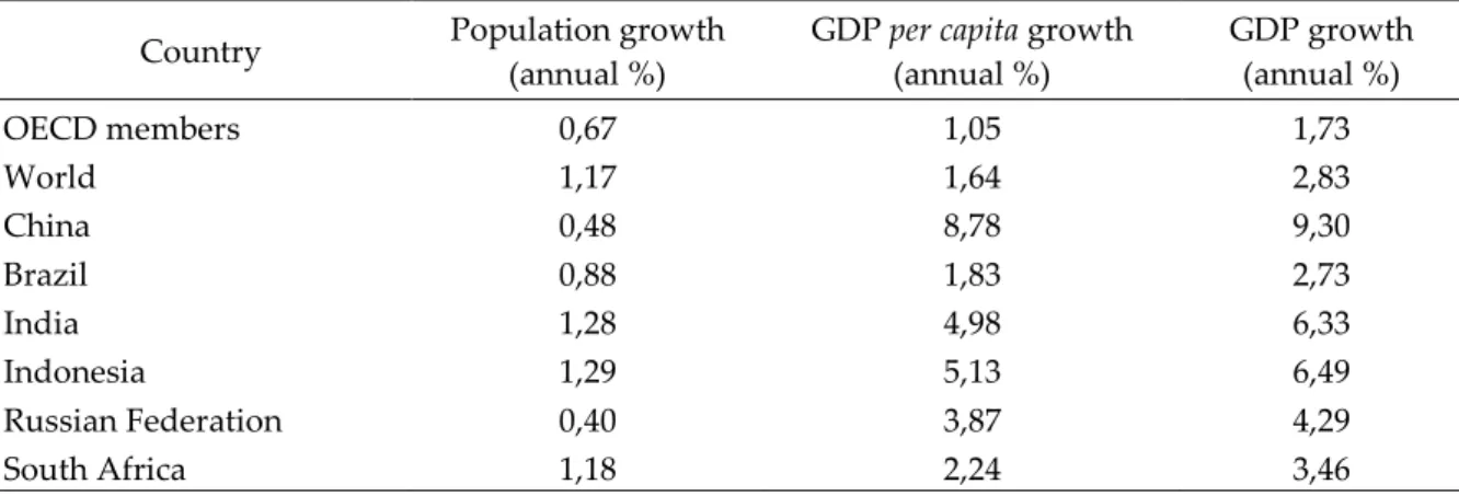
Deliktas and Balcilar (2005) estimated the relative technical efficiencies and efficiency change, technical change and TFP change in the transition economies for the period 1991-2000, using the stochastic frontier approach. They estimated a translog stochastic production function, where the output (GDP) of a country is assumed to be a function of two inputs, capital and labor. By using the Battese and Coelli (1995) time-varying inefficiency model, the authors were able to measure technical efficiency and technical change in the transition economies, and at the same time model technical inefficiency effects as a function of country-specific socioeconomic factors, liberalization and democratization indices, and time period under the Soviet Regime.
Pires and Garcia (2012) estimated and decomposed TFP change using SFA. They estimated a world production frontier for 75 countries for the period 1950-2000. Then they decomposed TFP change for a smaller sample of countries using the “Bauer-Kumbhakar” approach. TFP change is decomposed not only into technical efficiency change, scale effects and technical change, but also into allocative efficiency change. They concluded that productivity accounts for almost all the differences of growth between developed and developing countries and that allocative efficiency is responsible for a large part of them. In fact, their main contribution in relation to other SFA studies is showing that allocative efficiency plays an important role in the economic growth of nations.
Afonso and Aubyn (2013) used the DEA approach to compute Malmquist productivity indexes as well as the SFA analysis for a set of OECD countries for the periods 1970, 1980, 1990 and 2000, choosing GDP per worker as output and
three inputs – human capital, public physical capital per worker and private physical capital per worker – and an environmental variable related to governance. Results showed that (i) private capital is important for growth; (ii) public and human capital contribute positively for growth but they may not be statistically significant; (iii) government effectiveness is important to explain inefficiency, where better governance influences a country’s performance positively.
The estimation of relative inefficiencies and TFP growth, in chapter 3, will follow a pattern somewhat similar to the ones proposed by Deliktas and Balcilar (2005), Pires and Garcia (2012) and Afonso and Aubyn (2013). Similarly to Deliktas and Balcilar (2005), the stochastic frontier model used will be an adaptation of the Battese and Coelli (1995) time-varying inefficiency model. The adoption of this model allows for the inclusion of exogenous variables to explain differences in inefficiencies. The production technology used will be the translog production function, due to its flexibility. The decomposition of the TFP is based on a primal approach adapted from Kumbhakar and Lovell (2000). The main contribution of this analysis, in comparison to the one proposed by Deliktas and Balcilar (2002), is the enlargement of the sample of countries by including all OECD countries plus the emergent economies of Brazil, China, India, Indonesia, Russian Federation and South Africa, analyzed for a more recent period (2001-2011). Additionally, some of the determinants of productivity growth included in the analysis will be different and more likely to affect all countries in the world, although with different intensities. Consequently, this analysis is more easily projected/ extended to the rest of the world. This is due to the fact that the purpose of Deliktas and Balcilar (2002) was to explain relative efficiencies among transition economies and those economies are affected by variables that are less likely to affect other countries (for example, the time period under the Soviet Regime). The main contribution
of this analysis, in relation to the one proposed by Pires and Garcia (2012), is the fact that technical inefficiency effects are assumed to be a function of country-specific explanatory variables. Those variables help understand the reasons behind the differences in inefficiencies across countries. Our main contribution in relation to the empirical application of Afonso and Aubyn (2013) is the extension of the sample of countries to include all the OECD countries plus the emergent economies and the inclusion of a broader set of country-specific variables to explain cross-country differences in inefficiencies, such as the weight of agriculture in the economy, the role of trade, the business environment, innovation, governance, among others.
3. The Empirical Model
3.1 Stochastic Frontier Time-Varying Inefficiency Model
The idea of an inefficiency stochastic frontier production function discussed in chapter 2. is now applied to a macroeconomic scenario in which the 34-OECD countries plus the emergent economies of Brazil, China, India, Indonesia, Russian Federation and South Africa are the producers of output (e.g. real GDP at current PPPs per worker) using a set of inputs (e.g. human and physical capital per worker). Countries can then be thought of as operating on the frontier or below it. The distance between the observed output and the corresponding value on the frontier reflects the level of inefficiency of a country in a certain moment in time. Over time, a country can increase or decrease its level of inefficiency and “catch-up” to the frontier or even the frontier itself can move upwards or downwards, reflecting technical progress or regress, respectively. Additionally, a country can move along the frontier by changing the scale of operations and experiencing the effects of returns to scale. Thus, a country can experience output growth due to factor accumulation or productivity growth, where the last component results from the joint effects of technical efficiency change, technical change and scale change. The estimation and decomposition of productivity change will be performed under the stochastic frontier time-varying inefficiency model of Battese and Coelli (1995) and the Kumbhakar and Lovell (2000) primal approach discussed in subchapter 2.2.2. A brief presentation of the Battese and Coelli’ model will be provided before the presentation of the data and the estimated model.
Battese and Coelli (1995) proposed a stochastic frontier model for (balanced/unbalanced) panel data, in which the technical inefficiency effects are explicitly formulated as a function of a set of explanatory variables.
The authors started the presentation of the theoretical model by defining the stochastic frontier production function for panel data as:
( ) ( )
where
represents the production of the i-th DMU ( ) in the t-th
period ( );
is a (1 x k) vector of values of known functions of inputs of the production function associated with the i-th DMU in the t-th period; is a (k x 1) vector of unknown parameters to be estimated;
’s represent random errors assumed to be idd ( ),
independently distributed of the ’s;
’s are non-negative random variables associated with technical inefficiency of production and are assumed to be independently distributed, obtained by truncation at zero of the (
)-distribution;
is a (1 x m) vector of DMU-specific variables which may vary over time;
is a (m x 1) vector of unknown coefficients of the DMU-specific inefficiency variables.
The technical inefficiency effect, , in the stochastic frontier production
function ( ) is defined as:
where is the random variable defined by the truncation of the normal
distribution with zero mean and variance , such that the truncation point is , i.e., . These assumptions are consistent with the fact that the
’s are non-negative truncations of the ( )-distribution. The
inefficiency frontier model defined by equations ( ) and ( ) specifies the stochastic frontier production function (which can be Cobb-Douglas, translog or any other type) in respect to the observed levels of production and the ’s as a
function of explanatory variables, the ’s, and a vector of coefficients, . The ’s include variables that explain the shortfall of the observed levels of
production in relation to the corresponding stochastic frontier levels of production, ( ). Note that, when the vector of coefficients is the
null vector, the explanatory variables cannot explain inefficiency effects and the distribution would become the ( ) distribution truncated above at zero originally proposed by Aigner, Lovell and Schmidt (1977).
The technical efficiency measure for the i-th DMU in the t-th period is defined as the ratio of observed output to the corresponding stochastic frontier output:
( )
( )
( ) ( ) ( ) ( ) Since the technical inefficiency effects may vary over time and DMU’s, the fact that a DMU is more inefficient relative to another DMU in period t does not necessarily imply that the same will happen in the next period. Consequently, the ranking of DMU’s defined in terms of technical efficiency may change over time. Maximum Likelihood was the method used to estimate the parameters of the inefficiency model ( ) ( ). The likelihood function and its partial derivates with respect to the parameters of the model can be found in Appendix C.