TSPO: an autoML approach to time series forecasting

(1)

TSPO: An AutoML Approach to

Time Series Forecasting

Siem Morten Johannes Dahl

Dissertation presented as the partial requirement for

obtaining a Master's degree in Data Science and Advanced

Analytics

(2)

NOVA Information Management School

Instituto Superior de Estatística e Gestão de Informação

Universidade Nova de Lisboa

TSPO: An AutoML Approach to Time Series Forecasting

by

Siem Morten Johannes Dahl

Dissertation presented as the partial requirement for obtaining a Master's degree in Data

Science and Advanced Analytics

Advisor: Mauro Castelli, Piero Ferrarese

(3)

TSPO: An AutoML Approach to Time Series Forecasting

Copyright © Morten Dahl, Information Management School, NOVA University Lisbon. The Information Management School and the NOVA University Lisbon have the right, perpetual and without geographical boundaries, to file and publish this dissertation through printed copies reproduced on paper or on digital form, or by any other means known or that may be invented, and to disseminate through scientific repositories and admit its copying and distribution for non-commercial, educational or research purposes, as long as credit is given to the author and editor.

This document was created using the (pdf)LA_{TEX processor, based on the “novathesis” template[1], developed at the Dep. Informática of FCT-NOVA} [2].

(4)

Abstract

Time series forecasting is an essential tool in many fields. In recent years, machine learning has gained popularity as an appropriate tool for time series forecasting. When employing machine learning algorithms, it is necessary to optimise a machine learning pipeline, which is a tedious manual effort and requires time series analysis and machine learning expertise. AutoML (automatic machine learning) is a sub-field of machine learning research that addresses this issue by providing integrated systems that automatically find machine learning pipelines. However, none of the available open-source tools is yet explicitly designed for time series forecasting.

The proposed system TSPO (Time Series Pipeline Optimisation) aims at providing an autoML tool specifically designed to solve time series forecasting tasks to give non-experts the capability to employ machine learning strategies for time series forecasting. The system utilises a genetic algorithm to find an appropriate set of time series features, machine learning models and a set of suitable hyper-parameters. The optimisation objective is defined as minimising the obtained error, which is measured with a time series variant of k-fold cross-validation.

TSPOoutperformed the official machine learning benchmarks of the M4-Competition in 9 out of 12 randomly selected time series. TSPO captured the characteristics of all analysed time series consistently better compared to the benchmarks.

The results indicate that TSPO is capable of producing robust and accurate forecasts without any human input.

Keywords: Time Series Forecasting, Genetic Algorithms, Machine Learning, Time Series

Decomposition, Time Series Cross-Validation, Hyper-parameter Optimisation, Time Series Feature Engineering, autoML

(5)

Resumo

A previsão de séries temporais é uma importante ferramenta em muitas disciplinas. Nos últimos anos, a aprendizagem automática ganhou popularidade como ferramenta apropriada para a previsão de séries temporais. Ao utilizar algoritmos de aprendizagem automática, é necessário otimizar pipelines de aprendizagem automática, que é um esforço manual, tedioso e que requer experiência na área. O AutoML (aprendizagem automática automatizada) é um subcampo de aprendizagem automática que aborda esse problema, fornecendo sistemas integrados que encontram automaticamente pipelines de aprendizagem automática. No entanto, nenhuma das ferramentas de código aberto disponíveis é explicitamente destinada à previsão de séries temporais.

O sistema proposto TSPO (Time Series Pipeline Optimisation) visa fornecer uma ferramenta de aprendizagem automática projetada especificamente para resolver problemas de previsão de séries temporais. Dando a não especialistas a capacidade de utilizar estratégias de aprendizagem automática para previsão de séries temporais. O sistema utiliza um algoritmo genético para encontrar um conjunto apropriado de pipelines de séries temporais, modelos de aprendizagem automática e um conjunto de hiperparâmetros adequados. O objetivo da otimização é definido como a minimização do erro obtido, medido com uma variante da validação cruzada k-fold aplicada a séries temporais.

O TSPO superou os benchmarks oficiais de aprendizagem automática da competição M4 em 9 das 12 séries temporais aleatoriamente selecionadas. Além disso o TSPO capturou as características de todas as séries temporais analisadas melhor que os benchmarks. Os resultados indicam que o TSPO é capaz de produzir previsões robustas e precisas sem qualquer contribuição humana.

Palavras-chave: Previsão de séries temporais, algoritmos genéticos, aprendizagem automática,

decomposição de séries temporais, validação e otimização de parâmetros, engenharia de carac-terísticas de séries temporais, autoML

(6)

List of Figures

3.1 TSPOOverview . . . 7

3.2 Decomposition of Time Series M26778 . . . 9

3.3 Genetic Search Algorithm Scheme . . . 11

3.4 Example for 3-Fold Cross-Validation of Time Series M26778 . . . 14

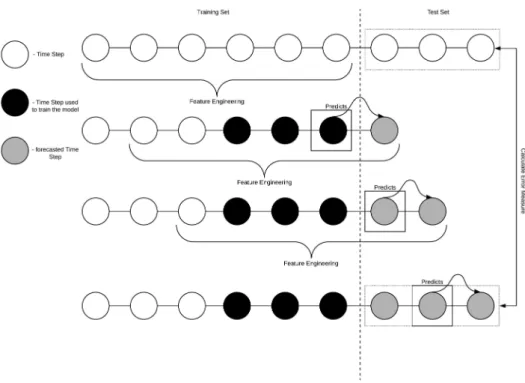
3.5 Recursive Strategy for Multi-Step Prediction . . . 16

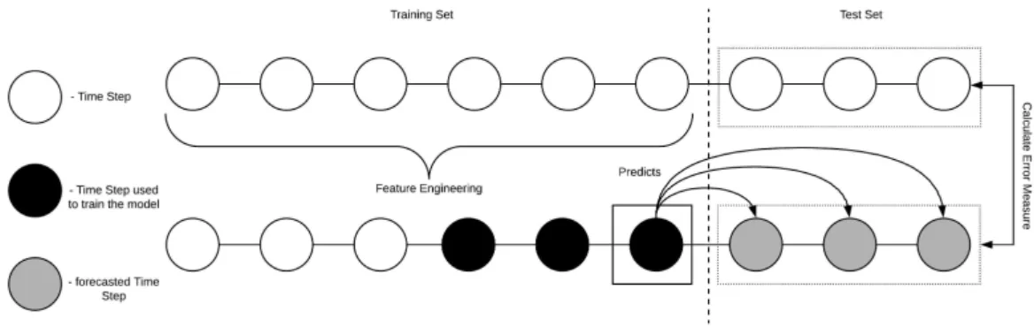
3.6 Multiple Output Strategy for Multi-Step Prediction . . . 17

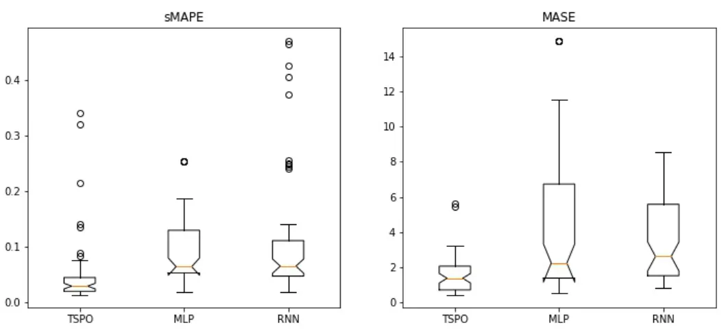
5.1 Boxplots of the sMAPE and MASE Distribution across all datasets . . . 21

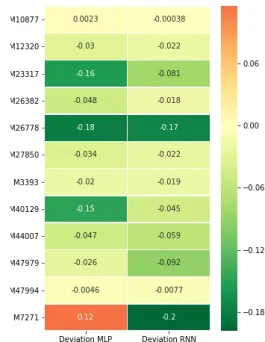
5.2 Heatmap of MASE Mean Deviations to TSPO . . . 23

5.3 Heatmap of sMAPE Mean Deviations to TSPO . . . 23

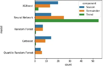
5.4 Algorithms used in Pipelines per Component . . . 24

(8)

List of Tables

3.1 Implementation of Machine Learning Algorithms . . . 15

A.1 Mean sMAPE for TSPO and Benchmarks . . . 37

(9)

Chapter 1

Introduction

Time series forecasting has gathered great attention ever since. The ability to look into the future drives the curiosity of researchers, analysts, and forecasters. In many different fields, such as meteorology, supply-chain optimisation, macro-economics, or finance, the impact of time series data is vast. In other domains, especially in business decision making, the use of data-driven support systems is increasing. Any decision made that employs resources of any kind benefits from having a rigorous approach to forecasting. It minimises misallocation, reduces wrong expectations, and gives a solid foundation to decision making processes.

Thus, there is an increasing and already high demand for robust, scalable, and accurate fore-casting tools. In recent years, machine learning algorithms gained popularity as an appropriate tool for time series forecasting. Statisticians and Data Scientists are now spending much time with the task of finding suitable features and models that provide accurate views into the future. Most machine learning algorithms require extensive pre-processing, feature selection, and hyper-parameter optimisation to be able to solve a time series forecasting task with a satisfying result. Analysts with forecasting, machine learning and domain expertise are relatively rare, which makes the engagement with appropriate and scalable time series forecasting tools expensive for organizations.

TSPO(Time Series Pipeline Optimisation) is a tool which aims at automating this task and thus, gives even non-experts in the field of machine learning the chance to employ machine learning to any given time series forecasting task. TSPO takes raw time series data and finds suitable machine learning approaches to extrapolate the time series into the future without any prior knowledge or any human input. The search is carried out by employing a Genetic Algorithm. There are recent developments and proposed systems in the area of automated machine learning. There are open-source tools, such as TPOT [59], auto-Weka [46] and auto-sklearn [27] and commercial tools, such as H2O Driverless AI. However, the afore-mentioned open-source tools do not provide appropriate support for time series forecasting, whereas TSPO is specifically designed to solve this task.

This thesis is structured in the following way: section 2 gives an overview of related work. Section3discusses the implementation and functionality of TSPO in detail. Section4

(10)

C H A P T E R 1 . I N T RO D U C T I O N

presents the experimental methodology to test the performance of TSPO against two benchmarks. Section5discusses the findings of the experimental phase, followed by section6, which states the limitations and gives proposals towards future work. The thesis is concluded in section7.

(11)

Chapter 2

Related Work

In this thesis, I will present a fully automated time series forecasting tool, which leverages a genetic algorithm to find suitable features, machine learning models and the respective hyper-parameters. The approach takes a raw time series, automatically decomposes it, extracts time series features for each decomposition and finds a model with fitting hyper-parameter. In this chapter, I will present related work for the three areas the proposed system touches. In2.1, I will discuss the current state of automatic machine learning. In2.2, I will present the topic of time series forecasting. In2.3, the final section of this chapter, I will review selected applications of genetic algorithms.

2.1 Automatic Machine Learning

The approach of the proposed system belongs to the field of automated machine learning (autoML). AutoML refers to solving a machine learning task in an automated way so that none (or very little) manual effort is required. AutoML aims at providing non-experts with the possibility of applying machine learning techniques to address a specific task without requiring prior technical or domain knowledge.

When trying to solve a machine learning task, it not only requires selecting an algorithm, it also requires setting up the hyper-parameters of the selected algorithm. Setting and tweaking hyper-parameters in the right way can - and often will - result in a better performing model. Generally speaking, there is no crystal-clear recipe for most algorithms to end up with a suitable pair of hyper-parameters. It is still a matter of intuition, domain-expertise and experience to tweak hyper-parameters in a way they result in a performant and robust model [14]. Research has also shown that a suitable set of hyper-parameters significantly increases the performance of models compared to most default settings [52,56].

The goal of most autoML approaches is to fully automatise the process of model selec-tion, hyper-parameter optimisaselec-tion, and feature selection. Previously, several approaches and strategies only tackled a subset of this process, whereas in recent years several fully automated approaches arose.

(12)

C H A P T E R 2 . R E L AT E D WO R K

of a set of possible hyper-parameters is applied to the task at hand. This brute force approach exhaustively tries every possible combination and returns the best fitting set of hyper-parameters. Random search is a different approach in which the possible hyper-parameters are randomly chosen and not predefined as in the grid search approach. Several studies have proven this approach to be more effective [4]. Other strategies for hyper-parameter optimisation involve gradient-search [2,63], evolutionary search [20,49,73] and Bayesian optimisation [23,45,65,

72].

With the recent development in the field of Bayesian optimisation, this approach gained more attention in the research community. Results suggest that hyper-parameter optimising algorithms in this domain are more effective than the brute force paradigm of grid search and random search. In some applications, these approaches even outperformed manual optimisation by domain experts[65].

Another aspect of autoML research is feature engineering. As manual feature engineering is a tedious and repetitive task, research has aimed to provide automatised tools. Three systems recently introduced to fulfil this task automatically are ExploreKit [43], the data science machine [42] and cognito [44]. The first uses meta-features extracted from previously known datasets and a machine learning-based algorithm to efficiently rank composed features, whereas the data science machinecan extract features from relational data sources leveraging deep feature synthesis. This approach was proven in several competitions to be more effective than the manual selection of appropriate features. Cognito explores various feature construction choices hierarchically and increases model accuracy through a greedy strategy.

In recent years several systems have been proposed that combine all three aspects of autoML: i.) model selection, ii.) hyper-parameter optimisation and iii.) feature engineering. Amongst others, TPOT [59], auto-Weka [46] and auto-sklearn [28] are integrated systems that produce pipelines to solve machine learning tasks and to solve the CASH (combined algorithm selection and hyper-parameter optimisation) problem.

The CASH problem refers to the task of not only finding a suitable set of hyper-parameters for a given model but enhancing this search with model selection, data pre-processing steps and feature engineering. Adding these steps enhances the search space for potential settings significantly and demands smarter choices in optimisation methods than brute force approaches such as grid search.

Auto-WEKAis built on top of the machine learning software WEKA and utilises its

imple-mentations of base learners, ensemble methods, meta-methods and feature selection methods. This system finds a suitable setting to solve the CASH problem using Bayesian optimisation for a given dataset. Kotthoff et al. found that this approach often outperforms standard model selection and hyper-parameter optimisation methods [46].

Similarly, auto-sklearn also relies on Bayesian optimisation to solve the CASH problem. This system is built on top of the well-known Python library scikit-learn [60] utilising its implementations for base learners, feature and data pre-processing methods. Feurer et al.

(13)

2 . 2 . T I M E S E R I E S F O R E CA ST I NG

enhance their system by taking knowledge gained from previous datasets into account and constructing ensembles from already evaluated models. This system was capable of winning 6 out of 10 competitions in the chalearn automl competition [35].

A different approach was proposed by Olson et al. Contrary to the former, the TPOT system does not rely on Bayesian optimisation but on genetic programming (GP). The system treats machine learning algorithms as GP-operators from which arbitrary long pipelines are constructed. The obtained results indicate that this system can outperform standard pipelines [59].

2.2 Time Series Forecasting

A time series is a sequence of historical measures of an observable variable y with an equal time interval [6]. There are many ways why time series are of interest. Generally, there are two main ideas when it comes to time series analysis: one is to understand the relationship between an input and an output variable, and the other is to be able to predict or forecast the future based on historical information [15]. In this thesis, I will focus on the latter. Time series forecasting is a crucial task in various fields of science such as economics, finance, business intelligence, meteorology and telecommunication [5]. Therefore, models able to produce robust and accurate forecasts are needed. One of the issues arising when creating a model that can fulfil such a task is the question of the forecasting horizon. Naturally, to create a forecast for one step into the future is already a challenge of its own. However, when talking about a multi-step forecasting approach, issues such as the accumulation of errors, increasing uncertainty and thus a reduced accuracy, are even more present [5]. Nevertheless, the presented system is dealing with an arbitrary number of steps ahead for a given time series and its functionalities are further discussed in section3.

Linear models dominated the forecasting domain for a long time. Up until the late 1970s, linear statistical methods such as ARIMA models were state-of-the-art. However, during that time, it became apparent that linear models are unable to adapt to many real-world applications [16]. So, several non-linear time series models were introduced. Amongst others, the threshold autoregressive model [68,69] and the autoregressive conditional heteroscedastic (ARCH) model [25] are examples of non-linear time series models. Despite these developments, the analytical study of non-linear time series forecasting is still in its infancy when compared to linear time series forecasting [5,16].

In the last three decades, machine learning approaches have reached the forecasting com-munity and are more regularly used in the context of time series forecasting. Amongst other techniques, neural networks are prevalent [47]. Neural networks, and machine learning in general, are data-driven and self-adaptive, which means only little a priori knowledge is required. These characteristics are different from traditional model-based approaches. Secondly, machine learning approaches are generalisable and, finally, they are non-linear [74]. Next to the usage of neural networks, several other machine learning techniques have been used for time series

(14)

C H A P T E R 2 . R E L AT E D WO R K

forecasting, i.e. gradient boosting [66], support vector machines [18] and more [1]. Additionally, there are many different ensemble methods for forecasting. For instance, Lee et al. combined ARIMA models, Neural Networks and genetic programming [48]. The work of Donate et al. is especially worth mentioning in this thesis as they are evolving neural networks with genetic algorithms for time series forecasting [21] and their results indicate that a genetic algorithm can find algorithms that solve time series forecasting tasks adequately.

2.3 Genetic Algorithms

Genetic Algorithms are a type of search and optimisation algorithm which belong to the class of evolutionary algorithms. This algorithm is biologically inspired by the evolution theory of Charles Darwin [33]. The core idea is that natural selection combined with variation will cause a population to evolve over time. In a search algorithm, a population of possible solutions to a given optimisation problem is evolved towards a better solution. In an iterative process, candidate solutions are evaluated and subsequently modified through genetic operators such as selection, crossover and mutation. This heuristic approach has been proven to work well in large search spaces with multiple local optima, and thus, it is predestined for the task at hand. In3.3, I give a more detailed description of the functionality of the search algorithm.

Over the past decades, various applications of genetic algorithms to optimisation problems were proposed. For instance in portfolio optimisation [9], bank loan decision [57], allocation of goods in shop shelves [8], supply chain management [37] and for the objective of this thesis most interestingly for hyper-parameter optimisation [20,49] and the optimisation of neural network architectures [30,61,62].

(15)

Chapter 3

TSPO

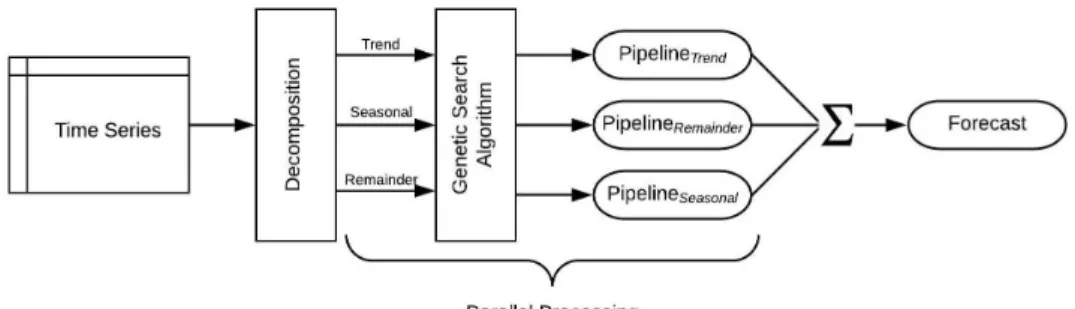
The name TSPO stands for Time Series Pipeline Optimisation. The goal is to find a suitable pipeline for a given time series. What is meant with a pipeline in this context is two-fold. First, the time series is decomposed into three components: a trend, seasonal and remainder component. For the sake of simplicity, a decomposition of a potential cycle component can be neglected. Secondly, for each of these components, TSPO focuses on finding a suitable selection of features, a suitable model and suitable hyper-parameters for the selected model. A full pipeline is considered to have three sets of selected features, three models, with each suitable hyper-parameters. When putting the decomposed series back together, the final forecast can be produced (see Fig. 3.1). In the following section, I will describe the process of finding these pipelines in detail and justify all relevant decisions. I will describe the decomposition in3.1. In

3.2, I will describe a pre-processing step. Next, I will explain the genetic search algorithm in

3.3by going into the details on how to evaluate candidate pipelines in3.4and how to engineer features in3.5.

3.1 Decomposition

The first step of the system is to perform a decomposition of the time series. The chosen tool to do this is the Singular Spectrum Analysis (SSA) [24, 34]. This tool decomposes a time

(16)

C H A P T E R 3 . T S P O

series (Y𝑡) into the sum of three individual components: a trend (T𝑡), a seasonal (S𝑡) and a

remainder component (R𝑡) at index t as given in (3.1). This step aims to deconstruct a seemingly

complex time series into small, interpretable components, which have different characteristics and, therefore, are easier to be forecasted individually.

Y𝑡 =T𝑡+ S𝑡+ R𝑡 (3.1)

The components are additive and independent of each other [36]. This characteristic is important for the design of the system as it allows for parallel processing of the pipeline search for each of the components.

In the first step of the decomposition algorithm, an embedding of the one-dimensional time series is performed. Embedding refers to mapping the one-dimensional time series into a multi-dimensional time series matrix, where each element consists of a lagged vector. The length of the lagged vector is determined by the window size, which is a parameter of the algorithm and is set to 4 in the current version of the system. The second step of the decomposition algorithm is to make a singular value decomposition (SVD) of the obtained matrix. The next step is to reconstruct the time series. This is done by grouping the decomposed matrix into a predefined number of groups (in the current version of the system the group parameter is set to 3 to be in line with (3.1)) and by subsequently applying diagonal averaging to the grouped matrix. For the proposed system, the implementation of SSA from the python package pyts [26] is used. Please refer to [24, 34] for a complete introduction to SSA. Figure 3.2shows exemplary a decomposition of one time series from the experimental phase (4).

3.2 Pre-Processing

At a first step, the decomposed data is scaled utilising the scikit-learn package [60] instance of the MinMaxScaler. Most machine learning algorithms require scaled data. Thus, to have a common approach, the entire data is scaled beforehand. There are two common ways to do that: the MinMaxScaler, which subtracts the minimum value and divides the result by the maximum subtracted by the minimum, and the StandardScaler, which takes the difference between the value and the mean value and divides the result by the standard deviation. The result of both approaches are features transformed to the same scale, whereas from the first, the values are bound between 0 and 1. As some algorithms, i.e. Neural Networks, require this bound [32], the MinMaxScalerwas the better choice. Even though this scaler is prone to outliers, it was used. Since there is currently no outlier treatment in the system, this must be considered a limitation. The subsequent step is to check the quality of the data in terms of format and appropriate length. At first, the system checks if the data was presented in a correct format, which is a pandasdataframe [53] with an index set to DateTime format. Furthermore, it checks how many time steps are present. As the system aims at producing robust and accurate forecasts, a certain requirement of time steps must be fulfilled. The minimum requirement is set by the following equation:

(17)

3 . 2 . P R E - P RO C E S S I NG

Figure 3.2: Decomposition of Time Series M26778

𝑛𝑡

(2 ∗ 𝑠 + 𝑡𝑎 ℎ 𝑒 𝑎 𝑑)

≥ 1 (3.2)

where 𝑛𝑡 is the total number of time steps, s refers to a natural seasonal cycle (i.e. for

monthly data it would be 12 as it corresponds to one year) and 𝑡𝑎 ℎ 𝑒 𝑎 𝑑 refers to the forecasting

horizon, meaning the steps into the future one would like to forecast. To prepare a time series to a supervised learning-like setting, features need to be extracted. Amongst other time series features, there are lagged values and moving averages. Both require a parameter: the lag size and the window size, respectively. If the user has not defined them differently, these parameters are set automatically in this step. If there are enough time steps both parameters are set to two seasonal cycles. For instance, both parameters would be set to 2 * 12 for a monthly time series, which corresponds to data from 2 full years. This allows the algorithm to capture the entire signal from the past two years and therefore capture eventual seasonal signals. If there are not enough time steps, the user must set these parameters. To prepare further for the feature engineering step, subsequent time series features are determined. This system utilises the tsfresh package [12], which allows extracting 36 time series characteristics. This results in 794 features, which is very prone to the curse of dimensionality. Hence, the features are supposed to be reduced. The tsfresh package includes a built-in feature filtering algorithm called fresh [13],

(18)

which relies on statistical hypothesis testing. This test is carried out, and only relevant features based on this algorithm are selected for the feature engineering step3.5. The last step of the pre-processing consists of cutting the time series into folds. To achieve the goal of producing robust forecasts, a variant of k-fold cross-validation is used for the evaluation of each pipeline.

3.3 Genetic Search Algorithm

Genetic Algorithms (GA’s) are a class of optimisation models that take the natural evolution process as a reference. Despite the existence of several variants of GA’s, instances share the following elements: a population of potential solutions, a selection method based on an assigned fitness score, crossover methods to redistribute information within the population and random variation in the form of mutation. The core of each GA is the fitness function as it incorporates the optimisation objective. This fitness function evaluates the goodness of fit for a candidate solution to the problem at hand and assigns a score to each of the candidate solutions. This score is used to compare the solutions. A well-designed fitness function is crucial for the success of the optimisation strategy.

Commonly, potential solutions or individuals are represented as bit strings. As this rep-resentation is not suitable for the problem at hand, the system uses a different reprep-resentation. The objective for the system is to find a pipeline including a set of features, a model, and a set of hyper-parameters. There are several issues to using bit strings as a representation: The model part could only contain one model, and hence there would be too many restrictions on assembling the bit string. Furthermore, the hyper-parameters are dependent on the model selection. Another issue with a bit string representation is that the hyper-parameters vary in terms of the data type. Some are floats with no bounds, some are integers, Boolean’s, or strings. The construction of a bit string that takes all this information into account would be too complex. Therefore, the system uses a different representation.

[F, M, P] (3.3)

As demonstrated in (3.3), the individual representation consists of three elements combined in a list-like object. The first element,F, is a set of feature id’s, that correspond to respective time series features. The second element,M, is a string of a model id, and the third element, P, corresponds to a hyper-parameter dictionary based on the selected model of the second element. This representation is flexible, since the first and second element are interchangeable, and not as complex as fitting all the information into a bit string. This form of representation carries several implications, which are described alongside the explanation of all genetic operators.

The first step of the genetic search algorithm is to initialise a random population. In the current state of the system, no specific initialisation function is used. The system randomly assembles individuals until the population size is reached. While individuals are randomly

(19)

3 . 3 . G E N E T I C S E A RC H A L G O R I T H M

(20)

generated, they are also evaluated. The evaluation process is described in section3.4. The default value for the population size is set to 10 but is adjustable by the user.

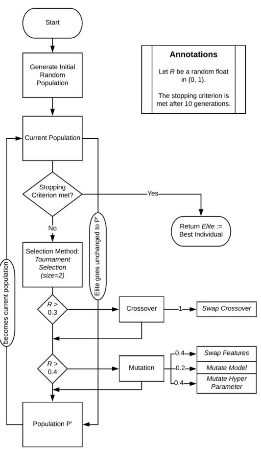
Now the actual evolutionary process starts. For n number of generations, the following process is repeated. The first step is to find the elite, the individual with the best fitness, in the current population. The elite goes unchanged to the next population to preserve information of at least one good solution. Now an inner loop takes place and is repeated until a new population is filled with individuals. At first, an individual is selected through a selection method. There are several different methods, however, this system relies on one of the most common methods called Tournament Selection. In this selection method, random individuals are drawn with replacement from the population until the tournament size is reached. From these drawn individuals, the one with the best fitness is selected. That means individuals with worse fitness are less likely to be drawn. However, with a very low probability, even the individual with the worst fitness has the chance to be selected, this is the stochastic characteristic of a GA.

The selected individual advances to the variation phase. With a certain probability, the crossover probability, crossover is carried out. If it is carried out, a second individual with the same process as described above is selected. Generally, there are several different crossover methods such as point-crossover, cycle-crossover and many more. This system uses a more simplistic approach. The crossover swaps the feature element of one individual with another so that one set of features is stacked to a different model and hyper-parameter. The resulting two offspring are either mutated with a mutation operator or go straight to the new population.

The mutation probability determines how likely it is that an individual mutates. The crossover operator shares characteristics between individuals of a population, mutation operators, however, explore yet unselected characteristics from the search space. Classical mutation methods contain shuffle-mutation, ball-mutation, or bit-flip. In this system, there are three different mutation methods present each touching one of the three elements of the individual representation.

1. Swap Features replaces 10% of the features with randomly selected ones.

2. Mutate Model exchanges the model with a random model from the search space. New hyper-parameters are assigned randomly, as well.

3. Mutate Hyper-Parameter ball mutates a randomly selected parameter. If the hyper-parameter is of type Boolean or string, it is chosen randomly.

The different mutation operators have different degrees of introducing new characteristics to the individual. Meaning, changing one hyper-parameter in a pipeline typically has less impact than exchanging an entire model and setting a new hyper-parameter at random. Therefore, each of the three mutation operators were assigned probabilities of being chosen. In the current version of the system, the probabilities are [0.4, 0.2, 0.4]. So, it is less likely, that the entire model is exchanged in this step rather than the introduction of different features or the exchange of a hyper-parameter. After the new population has reached the desired population size, the old population is deleted, and the evolutionary search continues until all generations are evolved.

(21)

3 . 4 . E VA LUAT I O N

The winning solution is the elite of the last generation. Figure3.3provides an overview of the genetic search algorithm.

3.4 Evaluation

The essential part of the genetic search algorithm is the way a candidate solution is evaluated. Since in the proposed system, the goal is to find suitable pipelines for a given forecasting task, this objective needs to be incorporated in the evaluation. In this section, I will discuss the evaluation in detail.

Each candidate solution is represented in the form explained in3.3. This representation is then translated into a pipeline and applied to the data at hand. Since we are dealing with a time series forecasting approach using machine learning models, the given time series needs to be translated into a supervised machine learning-like setting. Having this said, the evaluation is carried out following these steps:

1. The data is split in k-folds for validation based on the defined fold dictionary from the pre-processing step3.2.

2. A feature engineering is done for each fold based on the candidate features (First element of the representationF), and the data is split into a training and a test set.

3. A machine learning model using the chosen method (Second Element M) and the respective hyper-parameter (Third ElementP) is fitted using the training set of each fold. 4. Forecasts are created using the test set as an input for each of the models.

5. The produced forecast is then compared to the true values of the test set, and the error is computed based on a preselected error measure.

6. The fitness value is set, which corresponds to the average error of all folds.

The validation of a candidate pipeline is one of the most important aspects of this system. The goal is to produce pipelines with a high generalisation ability, meaning they overfit as least as possible and, thus, have predictive power.

A common practice in machine learning to detect overfitting and to measure the generalisation error is the utilisation of cross-validation. However, due to the serial correlation, which typically occurs in time series data, a traditional k-fold cross-validation strategy is impractical [17]. Usually, each of the folds become once the test set and serve all other times as the training set. Because of the serial correlation, this is generally not a favourable strategy for time series data. Even though some researchers propose this technique for purely autoregressive models [3]. A different strategy would be to use a classical hold-out-sample strategy, where the last part of a time series is used as a test set [67]. However, this strategy might not be able to detect overfitting accurately. There are also other common strategies, such as nested cross-validation [71]. The backdrop of this strategy is that it allows leakage between different folds.

(22)

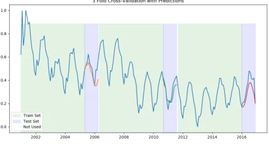
Figure 3.4: Example for 3-Fold Cross-Validation of Time Series M26778

So, the strategy of choice should prevent leakage between the folds and more importantly, between the training and the test set within each fold. The order of time steps needs to be respected, and no information about the test data can be in the training data. The used strategy is illustrated in Figure3.4. The entire data set is partitioned in folds. The fold size is determined by the maximum lag * 2 + the forecasting horizon. The number of folds is determined by the number of samples divided by the fold size, rounded down. The remaining samples that do not belong to a fold are used as a buffer between the folds to further prevent any leakage of information. For every fold, the test set is determined as the last datapoints with the size of the forecasting horizon. The usage of another validation split to use for further hyper-parameter optimisation was neglected as per the design of the system.

The following steps are executed per fold in a subsequent manner. The feature engineering is carried out, and the resulting dataset is split into a training and a test set. The length of the test set is determined by the forecasting horizon. The number of samples in the test set is equal to the steps ahead into the future. Please refer to3.5for a detailed description of the feature engineering step.

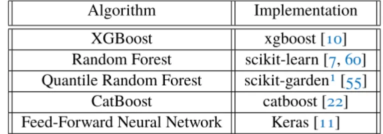
The next step is to fit a model to the training data set. In the current version of the system, there are five different machine learning models, that could be selected by the algorithm. Four tree-based algorithms are present in the system: A classical random forest, a quantile random forest, an extreme gradient boosting, and a categorical boosting algorithm. These algorithms have been proven to work well with time series forecasting problems [38,41,50,66].

There is also a classical feed-forward neural network with its architecture being a hyper-parameter. Neural networks have been proven to work well with time series forecasting. They appear to be especially good in capturing non-linear time series [1, 21, 48]. For the implementation of the algorithm, standard libraries are used and described in table3.1. Since time series forecasting is a regression problem all these methods, use the respective regressor

(23)

Algorithm Implementation XGBoost xgboost [10] Random Forest scikit-learn [7,60] Quantile Random Forest scikit-garden1[55]

CatBoost catboost [22] Feed-Forward Neural Network Keras [11]

Table 3.1: Implementation of Machine Learning Algorithms

implementation.

As a next step, these regressors need to be tested on unseen data. To do that, forecasts are generated for the steps ahead and compared to the true values. The system allows for forecasting multiple steps ahead, and therefore, the issue of producing a multiple steps ahead forecast must be considered. Several strategies exist, and I will discuss them in the following section.

As already mentioned in2.2the one step ahead forecasting problem can be written as a supervised learning approach such that an input matrix X consisting of past values of the time series is used as a training data set,

𝑋=           𝑦𝑁−1 𝑦𝑁−2 · · · 𝑦𝑁−𝑛−1 𝑦_𝑁₋₂ 𝑦_𝑁₋₃ · · · 𝑦_𝑁_−𝑛−2 . . . . . . . . . . . . 𝑦𝑛 𝑦𝑛−1 · · · 𝑦1           (3.4)

where N refers to current time step and n to the total number of samples in the time series and mapped to a scalar vector y

𝑦=           𝑦𝑁 𝑦_𝑁₋₁ . . . 𝑦𝑛+1           (3.5)

consisting of the respective time step ahead (N+1). For the sake of simplicity, features derived from past values are not mentioned in the equations throughout this chapter. For the one step forecast the forecast is generated from the values at the current time step, such that

ˆ𝑦𝑁+1= ˆ𝑓(𝑦𝑁, 𝑦𝑁−1,· · · , 𝑦𝑁−𝑛−1) (3.6)

where ˆ𝑓 refers to the trained regressor and ˆ𝑦 refers to the forecast. From this set up several possible strategies to perform a multi-step forecast can be derived. A multi-step forecasting can be considered when the periods to be forecasted exceed 1. So that the next H values [𝑦𝑛+1,· · · , 𝑦𝑁+𝐻], where H > 1, can be considered as the forecasting horizon or the steps ahead.

Three common strategies are: the recursive, the direct and the multiple output strategy. The recursive strategy uses a one step model and uses H times recursively the predicted previous value to forecast the next one. It trains a model ˆ𝑓 such that

(24)

Figure 3.5: Recursive Strategy for Multi-Step Prediction

ˆ𝑦𝑡+𝐻 = ˆ𝑓( ˆ𝑦𝑡+𝐻 −1, ˆ𝑦𝑡+𝐻 −2,· · · , 𝑦𝑡,· · · , 𝑦𝑡−𝑛+1) (3.7)

with t representing the current time step. Figure3.5provides an illustration of this strategy. This strategy is widely used, despite the known shortcomings of accumulating estimation errors. Since the input for the predictions are predictions itself, potential estimation errors are carried on into the future.

A different strategy is the direct strategy. In this strategy, H different models are trained, each having a different forecasting horizon. The benefit is that no predicted values are used to generate forecasts. However, there are as well several downsides to this approach. Firstly, there is no statistical dependency between the generated forecast, and secondly, the computational costs for training this many individual models are much higher. Figure3.6provides an illustration of this strategy.

The two previous strategies always consist of a single output. The underlying of the multiple output strategy (also known as Joint Strategy) is that the output is not a single scalar but a vector of forecasted values such as

[ ˆ𝑦𝑡+𝐻,· · · , ˆ𝑦𝑡+1] = ˆ𝑓(𝑦𝑛,· · · , 𝑦𝑁−𝑛+1) (3.8)

There are two benefits of this strategy: Firstly, unlike the direct strategy this strategy takes the stochastic dependencies between the different outputs into account, and secondly, this strategy does not accumulate a prediction error such as the recursive strategy. However, a downside is the reduced flexibility of the model. Using the direct or the recursive strategy, every forecasting

(25)

Figure 3.6: Multiple Output Strategy for Multi-Step Prediction

horizon could be chosen without much additional effort to adjust the models, whereas, with this strategy, the horizon is fixed [5]. Amongst others, there are two more hybrid strategies: the DirRec and the DIRMo strategy. They are not considered in the initial version of the system. In this system, the recursive strategy and the multiple output strategy are used. All tree-based algorithms use the recursive strategy, the feed-forward neural network uses a multiple output strategy. The reason why the multiple output strategy is only used for the neural network is that the tree-based models do not allow for multiple outputs, whereas the neural network is predestined for this approach as the output layer can be of arbitrary shape. These strategies are used over the direct strategies as they are computationally less expensive.

After the forecast is produced, it is compared to the true value, and the error is computed. The fitness (as described in3.3) of each candidate pipeline is its performance in this evaluation step. There are several error metrics implemented in the current state of the system, and the user is given the opportunity to select one of the predefined error measures or to pass a custom error metric. In the following section, I explain the predefined error metrics. The mean absolute erroris given by 𝑀 𝐴𝐸 = 1 𝑛 𝑛 Õ 𝑖=1 | (𝑦𝑡− ˆ𝑦𝑡) | (3.9)

where y corresponds to the true value, ˆ𝑦 to the forecasted value and n to the number of forecasted values. This nomenclature is used throughout this chapter. This metric takes the absolute error and averages it. A similar approach is the mean squared error, which takes instead of an absolute the squared error. It is given by

𝑀 𝑆 𝐸 = 1 𝑛 𝑛 Õ 𝑖=1 (𝑦𝑡− ˆ𝑦𝑡) 2 _(3.10)

These are quite common error metrics and used in various applications. However, they have several drawbacks such as being prone to outliers and their scale dependency [40,64].

Two different approaches use a percentage error. These approaches are the most common in forecasting [64] and are easier to compare against each other when having differently scaled

(26)

time series. Differently to the mean absolute percentage error given in3.11, the symmetric mean absolute percentage errorgiven in3.12has a lower and an upper bound [0, 200].

𝑀 𝐴𝑃 𝐸 = 1 𝑛 𝑛 Õ 𝑖=1 |𝑦𝑡 − ˆ𝑦𝑡 𝑦𝑡 | ∗ 100 (3.11) 𝑠 𝑀 𝐴𝑃 𝐸 = 1 𝑛 𝑛 Õ 𝑖=1 |𝑦𝑡− ˆ𝑦𝑡 𝑦_𝑡+ ˆ𝑦_𝑡| ∗ 200 (3.12) Another approach that is resistant to outliers is the mean absolute scaled error given in3.13. However, if all true values are equal, and hence the difference between them is 0, a division by 0 occurs [40,64], which is unfavourable and results in an error.

𝑀 𝐴𝑆 𝐸 = 1 𝑛 𝑛 Õ 𝑖=1 |𝑦𝑡 − ˆ𝑦𝑡| 1 𝑛−1 Í𝑛 𝑖=2|𝑦𝑖− 𝑦𝑖−1| (3.13) The experimental phase is carried out using the sMAPE error. The fitness value, in the end, is given by the error given from the selected error metric and averaged over all folds.

3.5 Feature Engineering

To be able to present a time series forecasting problem to a machine learning algorithm, features need to be extracted. ML algorithms need a labelled dataset in a form presented in3.4and

3.5. To achieve this, feature engineering is carried out. In the current version of the system, 4 different categories of features are extracted: lags, moving averages, datetime features and tsfreshfeatures.

Lags are previous time steps of a specific time point. The extraction of the lag values makes a given time point depending on previous time steps. Thus, the ML algorithm can catch signals from previous time steps. Moving averages take from a given time window the average. The system uses a maximum lag value and the window size parameter, which is set in the pre-processing step (3.2). From the provided dates in the original time series, datetime features are extracted. These consist of, i.e. week, month, quarter, and year. The tsfresh features are extracted by calling the python library.

(27)

Chapter 4

Experimental Methodology

The M4-Competition serves as a benchmark to understand the behaviour of the system and to demonstrate its capabilities. The M4-Competition is the 4th edition of the Makridakis challenge [51], a forecasting challenge that was first established in 1979. This edition was published in January 2018. This challenge was used as a benchmark, because, on the one hand, it provided accurate and clean data; on the other hand, this challenge had a strong emphasis on reproducibility [39]. Therefore, official benchmarks are available in a public GitHub repository

1. The challenge consisted of two sub-challenges, the first is to predict intervals, and the second is to produce point forecasts. The benchmarking of this thesis focuses on the latter. The proposed benchmarks by the M4-Competition consists of statistical benchmarks and ML benchmarks. To have a fair set-up, the ML benchmarks were used. They consist of a multi-layered perceptron and a recurrent neural network with both basic architecture and parametrisation as well as a basic pre-processing with detrending and deseasonalisation. Because the treatment of data and the chosen models are similar to the search space of TSPO, this benchmarking is suitable. The data used in the competition consist of a total of 100,000 time series. The time series have time intervals ranging from yearly to hourly and is distributed in 6 different domains (Micro, Industry, Macro, Finance, Demographic and other). Because of the high computational cost of finding a pipeline with TSPO, a subset of these time series was used for benchmarking. The subset used monthly data with two randomly chosen time series from each domain. The benchmarking was carried out in two steps. Over five replicas (seeds) TSPO searched for a suitable pipeline on each of the selected time series. The system was given 15 generations with a population size of 10. Considering the decomposition, TSPO evaluated 450 (15 generations * 10 individuals per population * 3 components) individual pipelines per replica using the cross-validation as discussed in3.4. To make the results of these pipelines comparable to the M4 benchmarks, the pipelines were fitted again on the dataset without cross-validation. A simple training and test set split was done, such that the test set consists of the forecasting horizon. The forecasting horizon was set to 12 steps ahead, which corresponds to one year ahead for the monthly data. The produced forecast is measured against the truth value to get an error score. Simultaneously, the two benchmark algorithms produced forecasts on the same datasets for the same forecasting

(28)

C H A P T E R 4 . E X P E R I M E N TA L M E T H O D O L O GY

horizon. The error measure resulting from this exercise are compared to the error measure from TSPO. Analogically to the M4-Competition, sMAPE and MASE are used as error measures.

(29)

Chapter 5

Experimental Results

To conclude whether the pipelines found by TSPO consistently perform better than the bench-marks, the obtained error metrics sMAPE and MASE from the 12 selected time series are compared. Error metrics are collected over five replicas of each time series, resulting in 60 error metrics. TSPO performed in 50 time series better than the benchmarks for the sMAPE error metric. In 49 time series TSPO obtained a better score for the MASE error metric. Figure5.1

shows the error distribution and tablesA.1andA.2show the mean errors for each time series. For both error measures, the mean is lower than the two benchmarks. For sMAPE, the extreme values of TSPO exceed the sMAPE values of MLP. Figures5.2and5.3show the mean deviation between TSPO and the two benchmarks. With regards to the RNN, TSPO performed better in all time series and for both error measures. With regards to the MLP, TSPO performed better in 10 out of 12 time series. In three time series (M23317, M26778, M40129), TSPO had a lower sMAPE score with a high magnitude (> 0.1), whereas MLP had a lower sMAPE score for M7271 with a high magnitude.

(30)

C H A P T E R 5 . E X P E R I M E N TA L R E S U LT S

ANOVA and the Friedman Test are carried out to test if these findings are statistically significant.

Within-subjectsANOVA is a standard statistical method to check whether multiple sample means differ or not [29]. The Null hypothesis tests if the sample means of each group are the same, and the observed variation is merely random [19]. In this context, the groups are the errors obtained from TSPO and the two benchmarks. The null hypothesis is rejected for sMAPE as well as for MASE at a 𝛼 = 0.05 significance level. Thus, the ANOVA provides evidence that the error measures follow a different distribution. The pairwise Tukey test [70] determines which groups (in this context, pipelines) are different. The test compares each group with each other and checks if the null hypothesis, samples of each group follow the same distribution, is to be rejected. The result shows that the error measures obtained from TSPO are significantly (𝛼 = 0.05) different from both benchmarks, whereas the error measures of the two benchmarks follow the same distribution. However, ANOVA requires several assumptions to be fulfilled, such as the samples being drawn from a normal distribution and equal variance [19]. Unfortunately, either one or the other assumption is violated for sMAPE and MASE. Therefore, the non-parametric Friedman test [31] is carried out to test further if the error measures of TSPO and the benchmarks are significantly different. This statistical method ranks the error measures of the pipelines in the range of [1, 3] and computes the average rank. The null hypothesis states that all pipelines are equivalent; thus, the mean rank is equal [19]. The null hypothesis is rejected on a 𝛼 = 0.05 significance level. Similarly to the pairwise Tukey test in ANOVA, the Nemenyi test [58] determines which groups differ. The result of the Nemenyi test and the previously described pairwise Tukey test reveal the same effect for both sMAPE and MASE: the error measures obtained from TSPO differ significantly from the error measures obtained by the two benchmarks. Analogically, the test comparing the two benchmarks fails to reject the null hypothesis, and thus, there is statistical evidence that they follow the same error distribution. The two statistical procedures ANOVA and the Friedman test independently concluded that the er-ror measures obtained by TSPO are significantly different from those obtained by the benchmarks.

The error measures show advantages in favour of TSPO. Nevertheless, these error metrics do not provide measures on the shape of the obtained forecasts. Figure5.5provides an overview of the generated forecasts, the benchmarks, and the actual time series values. When visually inspecting the generated forecasts, it gets apparent that the forecasts generated by the pipelines found by TSPO capture the shapes of the time series better than the benchmarks. Except for two cases (M7271, M26382), the overall trend was detected. The reason for this could be the feature engineering carried out by TSPO, which is more extensive compared to the benchmarks. Furthermore, the Singular Spectral Analysis used to decompose the time series could be a factor in a way that each component is better detected for TSPO than the benchmarks. Another aspect is the use of a k-fold cross-validation variant (refer to3.4) to evaluate candidate pipelines. This procedure provides pipelines with a high generalisation ability and, thus, with high predictive power. The likelihood of overfitting is reduced.

(31)

Figure 5.2: Heatmap of MASE Mean Deviations to TSPO

Figure 5.3: Heatmap of sMAPE Mean Deviations to TSPO

The pipelines mainly consist of the feed-forward neural network. Especially for the trend component, the neural network performed best. In 55 out of 60 cases, TS PO selected the Neural Network. This finding is in line with Ahmed et al. [1], who found an MLP performing best on the monthly M3 data set, the predecessor challenge of the M4-Competition. For the seasonal component, XGBoost appears to perform best. The least selected algorithms are random forest, quartile random forest, and cat boost.

Overall, TSPO appears to be a competitive system to find time series forecasting pipelines without any human input. The experimental results show that the obtained errors are significantly lower than the errors of the benchmarks. Furthermore, the forecasting pipelines are better in modelling and predicting the shapes of the analysed time series.

(32)

C H A P T E R 5 . E X P E R I M E N TA L R E S U LT S

(33)

(34)

Chapter 6

Limitations and Future Work

AutoML and hence TSPO rely on computationally intensive search strategies. These strategies require a high computational run-time, and hence for decent results, one has to wait for some time. For instance, Olson et al. [59] report 8h of run-time in their experimental approach. The runs carried out by TSPO took between 4h to 10h on a regular machine, and to get better results, a longer run-time could increase the performance. For practical use, this is a limitation. The computational costs are within the evaluation of a pipeline. Especially the feature engineering, in combination with the multi-step prediction is the bottleneck. A more performant implementation of this step could improve the run-time of TSPO significantly. One direction could be to enable the use of GPUs.

Another limitation is the choice of models in the search space. The current version of TSPO supports five different machine learning algorithms, as discussed in section3. The choice of algorithms could be enhanced by introducing more and different models. For instance, recurrent neural networks, especially LSTM’s, have been proven to work effectively for time series problems [54]. Furthermore, classical statistical approaches, such as ARIMA or exponential smoothing, could be introduced. As they require less training time than resource-intensive machine learning approaches, a research direction could be to find a good training time vs prediction accuracy trade-off. Like the previous argument, a shift from a pure genetic algorithm strategy towards a genetic programming paradigm could enhance the flexibility of pipelines. Similar to TPOT, the candidate solution, in this context, the pipeline, could be represented by a genetic programming tree. This would give TSPO the capability to evolve pipelines of arbitrary shape. In other words, the pipelines do not need to follow the current format as given in3.3.

The last stated limitation is the introduction of further hyper-parameter. The genetic algorithm itself introduces hyper-parameters such as tournament size, cross-over rate, and mutation rate – these hyper-parameters need to be optimised to achieve good results. Extensive research on the use of them could be fruitful to optimise the performance of TSPO. However, this research is computationally expensive, and the first stated limitation should be addressed first.

Lastly, I would like to give another proposal for future research. In the current state of TSPO, no prior knowledge of previous pipelines is incorporated in the search strategy. A warm start mechanism, which uses potentially suitable pipelines for specific time series problems, could

(35)

C H A P T E R 6 . L I M I TAT I O N S A N D F U T U R E WO R K

lead to an increase in performance. However, the issue of getting stuck in a local optimum (premature convergence) needs to be considered when pursuing this idea.

(36)

Chapter 7

Conclusion

Finding suitable machine learning pipelines for time series forecasting tasks poses a tedious and challenging effort and requires expertise in the field of time series forecasting and machine learning. Experts that combine both fields are relatively rare. The proposed system TSPO addresses this issue by providing an autoML approach for time series forecasting and enables non-expert practitioners to use machine learning capabilities without extensive technical and domain knowledge. Most open-source autoML systems do not tackle the specific demands of time series forecasting tasks.

The proposed system directs this issue by automatically performing a decomposition, extract-ing a set of relevant time series features, findextract-ing a suitable model and respective hyper-parameters for each of the obtained components. The system does these tasks by employing a genetic al-gorithm that independently evolves a pipeline for each component. The optimisation criterion of the genetic algorithm is to minimise the error of a multi-step forecast, which is obtained by utilising a time series variant of k-fold cross-validation. This method allows obtaining robust forecasts and, thus, addresses the issue of overfitting. The output of TSPO is a forecasting pipeline that can process most of the time series signals and produce robust forecasts. TSPO is capable of achieving this without any human input.

Empirical results show that TSPO outperforms the machine learning benchmarks of the M4-Competition in 9 out of 12 selected time series tasks. In all given time series, TSPO captures the shapes of each time series (i.e. the overall trend) consistently better.

The current implementation of the proposed system is computationally expensive. Future work may consequently focus on improving the run-time of the system. Furthermore, the optimal setting for the genetic algorithm hyper-parameter and the incorporation of prior knowledge may be subject to further research.

(37)

Bibliography

[1] N. K. Ahmed, A. F. Atiya, N. E. Gayar, and H. El-Shishiny. “An empirical comparison of machine learning models for time series forecasting.” In: Econometric Reviews 29.5-6 (2010), pp. 594–621.

[2] Y. Bengio. “Gradient-based optimization of hyperparameters.” In: Neural computation 12.8 (2000), pp. 1889–1900.

[3] C. Bergmeir, R. J. Hyndman, and B. Koo. “A note on the validity of cross-validation for evaluating autoregressive time series prediction.” In: Computational Statistics & Data Analysis120 (2018), pp. 70–83.

[4] J. Bergstra and Y. Bengio. “Random search for hyper-parameter optimization.” In: Journal of machine learning research13.Feb (2012), pp. 281–305.

[5] G. Bontempi, S. B. Taieb, and Y.-A. Le Borgne. “Machine learning strategies for time serie s forecasting.” In: European business intelligence summer school. Springer. 2012, pp. 62–77.

[6] G. E. Box, G. M. Jenkins, G. C. Reinsel, and G. M. Ljung. Time series analysis: forecasting and control. John Wiley & Sons, 2015.

[7] L. Breiman. “Random forests.” In: Machine learning 45.1 (2001), pp. 5–32.

[8] M. Castelli and L. Vanneschi. “Genetic algorithm with variable neighborhood search for the optimal allocation of goods in shop shelves.” In: Operations Research Letters 42.5 (2014), pp. 355–360.

[9] T.-J. Chang, S.-C. Yang, and K.-J. Chang. “Portfolio optimization problems in different risk measures using genetic algorithm.” In: Expert Systems with applications 36.7 (2009), pp. 10529–10537.

[10] T. Chen and C. Guestrin. “Xgboost: A scalable tree boosting system.” In: Proceedings of the 22nd acm sigkdd international conference on knowledge discovery and data mining. 2016, pp. 785–794.

[11] F. Chollet et al. Keras.https://keras.io. 2015.

[12] M. Christ, N. Braun, J. Neuffer, and A. W. Kempa-Liehr. “Time series feature extraction on basis of scalable hypothesis tests (tsfresh–a python package).” In: Neurocomputing 307 (2018), pp. 72–77.

(38)

B I B L I O G R A P H Y

[13] M. Christ, A. W. Kempa-Liehr, and M. Feindt. “Distributed and parallel time series feature extraction for industrial big data applications.” In: arXiv preprint arXiv:1610.07717 (2016).

[14] M. Claesen and B. De Moor. “Hyperparameter search in machine learning.” In: arXiv

preprint arXiv:1502.02127(2015).

[15] J. D. Cryer and N. Kellet. Time series analysis. Springer, 1991.

[16] J. G. De Gooijer and R. J. Hyndman. “25 years of time series forecasting.” In: International journal of forecasting22.3 (2006), pp. 443–473.

[17] M. L. De Prado. Advances in financial machine learning. John Wiley & Sons, 2018. [18] C. Deb, F. Zhang, J. Yang, S. E. Lee, and K. W. Shah. “A review on time series forecasting

techniques for building energy consumption.” In: Renewable and Sustainable Energy

Reviews74 (2017), pp. 902–924.

[19] J. Demšar. “Statistical comparisons of classifiers over multiple data sets.” In: Journal of Machine learning research7.Jan (2006), pp. 1–30.

[20] C. Di Francescomarino, M. Dumas, M. Federici, C. Ghidini, F. M. Maggi, W. Rizzi, and L. Simonetto. “Genetic algorithms for hyperparameter optimization in predictive business process monitoring.” In: Information Systems 74 (2018), pp. 67–83.

[21] J. P. Donate, X. Li, G. G. Sánchez, and A. S. de Miguel. “Time series forecasting by evolving artificial neural networks with genetic algorithms, differential evolution and estimation of distribution algorithm.” In: Neural Computing and Applications 22.1 (2013), pp. 11–20.

[22] A. V. Dorogush, V. Ershov, and A. Gulin. “CatBoost: gradient boosting with categorical features support.” In: arXiv preprint arXiv:1810.11363 (2018).

[23] K. Eggensperger, M. Feurer, F. Hutter, J. Bergstra, J. Snoek, H. Hoos, and K. Leyton-Brown. “Towards an empirical foundation for assessing bayesian optimization of hy-perparameters.” In: NIPS workshop on Bayesian Optimization in Theory and Practice. Vol. 10. 2013, p. 3.

[24] J. B. Elsner and A. A. Tsonis. Singular spectrum analysis: a new tool in time series analysis. Springer Science & Business Media, 2013.

[25] R. F. Engle. “Autoregressive conditional heteroscedasticity with estimates of the variance of United Kingdom inflation.” In: Econometrica: Journal of the Econometric Society (1982), pp. 987–1007.

[26] J. Faouzi and H. Janati. “pyts: A Python Package for Time Series Classification.” In:

Journal of Machine Learning Research21.46 (2020), pp. 1–6. u r l:http://jmlr.org/

papers/v21/19-763.html.

[27] M. Feurer, A. Klein, K. Eggensperger, J. Springenberg, M. Blum, and F. Hutter. “Efficient and robust automated machine learning.” In: Advances in neural information processing systems. 2015, pp. 2962–2970.

(39)

[28] M. Feurer, A. Klein, K. Eggensperger, J. T. Springenberg, M. Blum, and F. Hutter. “Auto-sklearn: efficient and robust automated machine learning.” In: Automated Machine

Learning. Springer, 2019, pp. 113–134.

[29] R. A. Fisher. “Statistical methods and scientific inference.” In: (1956).

[30] M. Fridrich. “Hyperparameter optimization of artificial neural network in customer churn prediction using genetic algorithm.” In: Trends Economics and Management 11.28 (2017), pp. 9–21.

[31] M. Friedman. “A comparison of alternative tests of significance for the problem of m rankings.” In: The Annals of Mathematical Statistics 11.1 (1940), pp. 86–92.

[32] A. Géron. Hands-On Machine Learning with Scikit-Learn, Keras, and TensorFlow: Concepts, Tools, and Techniques to Build Intelligent Systems. O’Reilly Media, 2019. [33] D. E. Goldberg. “Genetic algorithms in search, optimization and machine learning.” In:

Reading: Addison-Wesley, 1989(1989).

[34] N. Golyandina and A. Zhigljavsky. Singular Spectrum Analysis for time series. Springer Science & Business Media, 2013.

[35] I. Guyon, I. Chaabane, H. J. Escalante, S. Escalera, D. Jajetic, J. R. Lloyd, N. Macià, B. Ray, L. Romaszko, M. Sebag, A. Statnikov, S. Treguer, and E. Viegas. “A brief Review of the ChaLearn AutoML Challenge: Any-time Any-dataset Learning without Human Intervention.” In: Proceedings of the Workshop on Automatic Machine Learning. Ed. by F. Hutter, L. Kotthoff, and J. Vanschoren. Vol. 64. Proceedings of Machine Learning Research. New York, New York, USA: PMLR, 2016, pp. 21–30. u r l:

http://proceedings.mlr.press/v64/guyon_review_2016.html.

[36] H. Hassani. “Singular spectrum analysis: methodology and comparison.” In: (2007). [37] A. Hiassat, A. Diabat, and I. Rahwan. “A genetic algorithm approach for

location-inventory-routing problem with perishable products.” In: Journal of manufacturing systems42 (2017), pp. 93–103.

[38] Y. Hong, J. Zhou, and M. A. Lanham. “Forecasting Intermittent Demand Patterns with Time Series and Machine Learning Methodologies.” In: (2018).

[39] R. J. Hyndman. “A brief history of forecasting competitions.” In: International Journal of Forecasting36.1 (2020), pp. 7–14.

[40] R. J. Hyndman and A. B. Koehler. “Another look at measures of forecast accuracy.” In: International journal of forecasting22.4 (2006), pp. 679–688.

[41] M. J. Kane, N. Price, M. Scotch, and P. Rabinowitz. “Comparison of ARIMA and Random Forest time series models for prediction of avian influenza H5N1 outbreaks.” In: BMC bioinformatics 15.1 (2014), p. 276.

[42] J. M. Kanter and K. Veeramachaneni. “Deep feature synthesis: Towards automating data science endeavors.” In: 2015 IEEE International Conference on Data Science and

(40)

[43] G. Katz, E. C. R. Shin, and D. Song. “Explorekit: Automatic feature generation and selection.” In: 2016 IEEE 16th International Conference on Data Mining (ICDM). IEEE. 2016, pp. 979–984.

[44] U. Khurana, D. Turaga, H. Samulowitz, and S. Parthasrathy. “Cognito: Automated feature engineering for supervised learning.” In: 2016 IEEE 16th International Conference on

Data Mining Workshops (ICDMW). IEEE. 2016, pp. 1304–1307.

[45] A. Klein, S. Falkner, S. Bartels, P. Hennig, and F. Hutter. “Fast bayesian opti-mization of machine learning hyperparameters on large datasets.” In: arXiv preprint

arXiv:1605.07079(2016).

[46] L. Kotthoff, C. Thornton, H. H. Hoos, F. Hutter, and K. Leyton-Brown. “Auto-WEKA: Automatic Model Selection and Hyperparameter Optimization in.” In: Automated Ma-chine Learning: Methods, Systems, Challenges(2019), p. 81.

[47] B. Krollner, B. J. Vanstone, and G. R. Finnie. “Financial time series forecasting with machine learning techniques: a survey.” In: ESANN. 2010.

[48] Y.-S. Lee and L.-I. Tong. “Forecasting time series using a methodology based on autoregressive integrated moving average and genetic programming.” In:

Knowledge-Based Systems24.1 (2011), pp. 66–72.

[49] S. Lessmann, R. Stahlbock, and S. F. Crone. “Optimizing hyperparameters of support vector machines by genetic algorithms.” In: IC-AI. 2005, pp. 74–82.

[50] J. R. Lloyd. “GEFCom2012 hierarchical load forecasting: Gradient boosting machines and Gaussian processes.” In: International Journal of Forecasting 30.2 (2014), pp. 369– 374.

[51] S. Makridakis, E. Spiliotis, and V. Assimakopoulos. “The M4 Competition: 100,000 time series and 61 forecasting methods.” In: International Journal of Forecasting 36.1 (2020), pp. 54–74.

[52] R. G. Mantovani, T. Horváth, R. Cerri, J. Vanschoren, and A. C. de Carvalho. “Hyper-parameter tuning of a decision tree induction algorithm.” In: 2016 5th Brazilian Confer-ence on Intelligent Systems (BRACIS). IEEE. 2016, pp. 37–42.

[53] W. McKinney et al. “pandas: a foundational Python library for data analysis and statistics.” In: Python for High Performance and Scientific Computing 14.9 (2011).

[54] S. McNally, J. Roche, and S. Caton. “Predicting the price of bitcoin using machine learning.” In: 2018 26th Euromicro International Conference on Parallel, Distributed

and Network-based Processing (PDP). IEEE. 2018, pp. 339–343.

[55] N. Meinshausen. “Quantile regression forests.” In: Journal of Machine Learning Research 7.Jun (2006), pp. 983–999.

[56] G. Melis, C. Dyer, and P. Blunsom. “On the state of the art of evaluation in neural language models.” In: arXiv preprint arXiv:1707.05589 (2017).