1
A Work Project, presented as part of the requirements for the Award of a Master’s Degree in Finance from the NOVA – School of Business and Economics.
THE IMPACT OF IDIOSYNCRATIC AND SYSTEMATIC SHORT-SELLING ON RETURN PREDICTABILITY
João Santos De Freitas Quintia Delgado 24600
A Project carried out on the Master’s in Finance Program, under the supervision of: Melissa Prado
2
THE IMPACT OF IDIOSYNCRATIC AND SYSTEMATIC SHORT-SELLING ON RETURN PREDICTABILITY
Keywords:
Short-selling,
short interest, stock returns, firm-specific, return predictability, idiosyncratic, systematicAbstract
This paper analyses the impact of idiosyncratic and systematic short-selling in terms of return predictability. We have used different estimation methods for each type of short-selling, in doing so we were able to achieve higher consistency in our results.
The way information is processed and flows was subject to scrutiny in order to understand how short-sellers behave according to information signals.
Idiosyncratic short-selling has shown to be a more reliable source of information at predicting future returns than systematic shorting, despite the lower impact on returns, idiosyncratic short-selling shows more consistent results.
3
Table of Contents
I. Introduction ... 4
II. Literature Review ... 5
III. Methodology ... 10
IV. Empirical Analysis ... 11
4.1 Idiosyncratic effects over returns ... 11
4.1.1 Pooled OLS ... 11
4.1.2 Fixed-Effects ... 13
4.2 Systematic effect over returns ... 16
4.2.1 Pooled OLS ... 16
4.2.2 Fixed-Effects ... 17
4.3 Analysis of Residuals ... 19
V. Conclusion ... 22
4
I.
Introduction
Short-selling is a sale of a security by an investor who does not own the security. The short- seller borrows the security and is charged the loan fee that consists in the interest for the loan of the respective security. The motivation behind this procedure is the belief that the price of the security will decline and the seller is able to buy it back at a lower price.
The aim of this project is to study whether the levels of short interest which is the amount of shares sold short but not yet covered is able to forecast stock returns. As increased levels of short interest suggest a future decline in stock prices several questions emerge: The literature has demonstrated short interest to be informative about future returns, however is not particularly clear where short-sellers get their information from, therefore we should ask what information are short-sellers getting? Is this information based on overall market news or is it specific to firms and industries?
I will attempt to demonstrate that short interest does have an impact on subsequent stock returns, therefore I differentiate systematic shorting from the non-systematic (idiosyncratic) part. The first corresponds to the overall market shorting and the later refers to the firm-specific short-selling.
Following Comerton-Forde, et al. (2015) that use different metrics to assess short-selling: short flow that is more likely to capture short term technical trading, in contrast to short interest that appears to reflect the sentiment regarding the long-term prospects of a stock. The main purpose will be to understand how short-sellers process information and what they do with it, by comparing systematic shorting with idiosyncratic I will differentiate two types of short-sellers and filter the way information is perceived and which type is being used.
As a result, I expect idiosyncratic shorting to have a significant effect in predicting future stock returns, in other words I will attempt to demonstrate that short-sellers act on firm-specific
5
information and as consequence are able to forecast future returns. On the other hand, it is expected systematic shorting to have lower predictive ability of returns, mainly due to the less informed nature of those shorts and ambiguous acquisition of information.
The project will be organised in the following way: firstly, a relevant literature review on the topic will be provided; followed by the methodology adopted during data processing; then an empirical analysis of the results achieved and finally a conclusion and future research will be suggested.
II.
Literature Review
Return predictability and short-selling have been a matter of study in the literature, several authors attempt to explain the performance of stock prices using predictors to forecast the behaviour of future returns.
Arguably one of the most well-known and used variables is short interest, considered to be the strongest predictor of stock returns. Rapach, Ringgenberg and Zhou (2016) find evidence that the predictive power of aggregate short interest is capable of enduring a sample period from 1973-2014 and results from its ability to predict future cash flow news.
In a study Callen and Fang (2015) observed the impact of short interest on stock price and crash risk, finding robust evidence that short interest is positively related to one-year ahead stock price crash risk, consistent with the view that short-sellers are able to detect bad news in the firms they short. The evidence suggests that the positive relation between short interest and future stock price crash is more persistent in firms with weak governance monitoring mechanisms, excessive risk taking behaviour and high information asymmetry between managers and shareholders.
The popular Wall Street view that short interest is a bullish signal because it represents latent demand, which will convert eventually into the actual purchase of shares covered by the short position is challenged by Desai, et al. (2002). They found that the abnormal return for firms
6
with short interest of at least 2.5% to be negative 76 basis points per month, while the corresponding abnormal return for firms with short interest of at least 10% is negative 113 basis points per month, concluding that high levels of short interest convey negative information, followed by subsequent poor stock market performance, being consistent with bearish signals. Future abnormal returns decline monotonically with the level of short interest, Dechow, et al. (1999) show that firms with zero short positions, the average one year ahead abnormal return is 2.3%, while firms with over five percent shorted, the average abnormal return is -11.9%. They suggest that large short positions are more likely to represent a consensus among short-sellers that a stock is overpriced.
Moreover, when combining different size factors of equally-weighted and value-weighted portfolios with short interest Asquith, Pathak and Ritter (2005) find that high short interest stocks tend to be tilted towards growth stocks in respect to value-weighted portfolios. Small-cap stocks are observed to be among the highly shorted ones while equally-weighted portfolios underperform more often value-weighted portfolios. These authors demonstrated that the only class of stocks consistently producing negative abnormal returns are small-cap stocks with extremely high short interest ratios. They reveal that high short interest stocks tend to have increased systematic risk and positively covary with small stocks.
In parallel with the previous findings, Au, Doukas and Onayev (2008) associate low short interest stocks with higher idiosyncratic risk, suggesting that could be a possible explanation of why these stocks are overvalued relative to high short interest ones, as high idiosyncratic risk would result in an imperfectly hedged position. Short-sellers would consequently avoid low short interest stocks and leading to its consequently overvaluation. The fact that short-sellers under allocate capital to such stocks, they tend to earn large abnormal returns, this suggests low short interest stocks earn higher returns because of higher arbitrage costs.
7
A major study by Diamond and Verrecchia (1987) states that an unexpected increase in short interest in a security is bad news, once it reveals that more of the sell orders were short-sales than previously expected, an unexpected increase in short-interest in a stock would predict a future price decline even if short interest were not announced to the public, because it would still reveal private information. Some price reaction could occur in-between short interest measurement and announcement as some private information becomes public over that brief period.
Short-sellers would be mostly interested in shorting stocks that will have near term price decline, avoiding stocks that will have near time price increase, if short-sellers are better informed it is expected that we find significant increases in short interest prior to extreme negative returns than for stocks with extreme positive returns (Best, Best and Mercado-Mendez 2008). They concluded short-sellers may be able to anticipate some negative news events as evidenced by the changes in short interest surrounding certain events that cause large negative returns.
If we are to rely on the view that short interest contains information about future market returns, we are to expect higher values of short interest index to predict lower future returns. In sample tests show that a one-standard-deviation increase in short interest index corresponds to a six to seven percent increase in the future annualized market excess return (Rapach, Ringgenberg and Zhou 2016). They observed that the strong performance of short interest as an indicator relates to the Global Financial Crisis, showing that aggregate stock return predictability and the associated utility gains tend to be particularly sizable around periods of severe economic recessions, concluding short interest to offer modest gains during “normal” times and striking gains during periods of macroeconomic stress.
The up-tick rule requires that the last sale must have been at a higher price than the sale preceding it before a share can be short sold, the lack of such rules in the UK enables short
8
interest to build up relatively quickly, therefore subsequent returns are informative (Mohamad, et al. 2013). In their study on the UK market the authors find that investors do react to the disclosure of a large increase in short interest and these large increases are followed by periods of strong abnormal returns for valuation shorts.
Month-to-month movements of short interest are positively related to returns, months with increases in short interest experience returns 3-4% greater than months with drop in short interest, security returns in the month following an increase in short interest are 0-1% greater than security returns in the month following a decrease in short interest (Brent, Morse and Stice 1990).
The association between short interest and prior months’ returns provides some support for the use of short sales for speculation. In contrast previous findings indicate that stocks with very high short interest from one month to another have already experienced during the previous month itself excess returns greater than other stocks by 4.1% per month on average, pointing no relationship between short interest increases in month 𝑡 − 1 to month 𝑡 and excess returns in months 𝑡 − 2, 𝑡 or 𝑡 + 1 (Hurtado-Sanchez 1978).
Many studies focus on subsequent returns as a result of current short-selling, however it is important to acknowledge that short-sellers are trading on short-term overreaction, a five-day return of 10% results in an increase in short-selling as a fraction of daily share volume 3.71 (2.71) percentage points for NYSE (Nasdaq) stocks.
The evidence suggests that shorting increases after periods of positive returns, days with considerably buying pressure and days of asymmetric information where traders act as liquidity providers and risk-bearing services (Diether, Lee and Werner 2008).
However, some authors disagree with the idea that short interest has any validity as an indicator. Biggs (1966) indicates a merely “coincidental validity”, attributing no meaningful correlation between the short interest trend theory and the price action of stocks, suggesting
9
investors should rely on fundamental company analysis rather than short interest. Under the same line of thought, Hurtado-Sanchez (1978) consider short interest to not affect current or future stock prices but admits short-sales stabilize the stock market by making stock returns depend more closely on the stocks’ risk and reducing the size of the stocks’ excess returns.
The capacity of short-sellers to process information and the levels of “informedness” is analysed by Chakrabarty and Shkilko (2013). The authors show that the superiority of information that short-sellers possess may be due to insider sales, their ability to analyse visible order flows allows them to identify disturbances in the supply of shares created by the often large insider sales.
On insider sales days short-sales by non-market makers increase by 26.11% and short-sales by market makers increase at least 83.13% (Chakrabarty and Shkilko 2013). They concluded that short-selling subsequent to insider transactions is informed rather than speculative.
Under the same line of thought, Blau, DeLisle and Price (2015) find that short-sellers rely on soft information in earnings announcements conference calls as relevant information for valuing stocks. The tone of communication is crucial for information acquisition as short-sellers trade against inflated language (inflated talks), thus short trades after conference calls are predictive of negative returns (Blau, DeLisle and Price 2015).
Systematic market shorting is considered to be a less informed way of short-selling, Engelberg, Reed and Ringgenberg (2012) found that market makers’ trades to be not well informed and their short sales to be associated with positive future returns on news days. On the other hand idiosyncratic short-selling is believed to be more informed, as short-sellers have industry and firm preferences that they analyse and try to understand (Huszár, Tan and Zhang 2016).
10
III.
Methodology
The data was accessed by WRDS website in which CRSP provided monthly data on North American stock returns, monthly frequency short interest data on those same stocks was obtained via Compustat database. The sample period observed ranges from 28th February 1990 to 31st October 2013 organised in an unbalanced panel data, comprising n=8,595 stocks (the cross-sectional component) across T=202 time periods (time series component) with a total N=nT=535,912 observations. Some missing values were neglected and due to the absence of short interest in some periods, returns and short interest data were adjusted for matching purposes.
The short interest ratio (𝑆𝐼𝑅𝑖,𝑡) was obtained as 𝑆𝐼𝑅𝑖,𝑡 = 𝑆ℎ𝑎𝑟𝑒𝑠 𝑂𝑢𝑡𝑠𝑡𝑎𝑛𝑑𝑖𝑛𝑔×1000𝑆ℎ𝑜𝑟𝑡 𝐼𝑛𝑡𝑒𝑟𝑒𝑠𝑡 and the total short interest (𝑇𝑜𝑡𝑆𝐼𝑅𝑡) was computed in the following way: 𝑇𝑜𝑡𝑆𝐼𝑅𝑡 = ∑𝑛 𝑆𝐼𝑅𝑖,𝑡
𝑖=1 .
The variable 𝐿𝑜𝑔1𝑅𝑒𝑡𝑖,𝑡 corresponds to the stock returns, having been eliminated the extreme values when 𝑅𝑒𝑡𝑖,𝑡 > 1000. In order to stabilize the series a new variable was
generated in which a logarithm was applied to the returns plus one: 𝑙𝑜𝑔1𝑅𝑒𝑡𝑖,𝑡 = 𝑙𝑜𝑔(1 + 𝑅𝑒𝑡𝑖,𝑡).
Different models have been estimated using a two-step estimation.
𝑆𝐼𝑅𝑖,𝑡 = 𝛽0+ 𝛽1𝑇𝑜𝑡𝑆𝐼𝑅𝑡+ 𝜀𝑖,𝑡 (1) 𝑆𝐼𝑅𝑖,𝑡 = 𝛽0+ 𝛽1𝑇𝑜𝑡𝑆𝐼𝑅𝑡+ 𝛽2𝑆𝑀𝐵𝑡+ 𝛽3𝐻𝑀𝐿𝑡+ 𝜀𝑖,𝑡 (2)
In a second equation I add for robustness purposes Fama and French’s dynamic factors of size, differential returns of small minus big market capitalization stocks 𝑆𝑀𝐵𝑡 and value, high book-to-market portfolio returns minus a low book-to-market stocks 𝐻𝑀𝐿𝑡. Ang (2014) considers these factors to reflect macro risk and to capture size and value premiums.
The methodology consists in a two-step stage estimation procedure: i) estimate the regression for 𝑆𝐼𝑅𝑖,𝑡 and storing the residuals 𝜀𝑖,𝑡 and fitted values 𝑆𝐼𝑅̂ ; ii) regress the returns 𝑖,𝑡 𝑙𝑜𝑔1𝑅𝑒𝑡𝑖,𝑡 at time t with the residuals 𝜀𝑖,𝑡 and 𝑆𝐼𝑅̂ (of the previous period). 𝑖,𝑡−1
11
The predictability of returns with short-selling information will be evaluated in Equations (3) and (4).
𝑙𝑜𝑔1𝑅𝑒𝑡𝑖,𝑡 = 𝛾0+ 𝛾1𝜀𝑖,𝑡−1+ 𝑢𝑖,𝑡 (3)
𝑙𝑜𝑔1𝑅𝑒𝑡𝑖,𝑡 = 𝛼0+ 𝛼̂ 𝑆𝐼𝑅1 𝑖,𝑡−1+ 𝑢𝑖,𝑡 (4)
Different estimation methods were used throughout the process, both Equations (1-2) were estimated by Pooled OLS and Fixed-Effects while Equations (3-4) have been estimated by Pooled-OLS, Fixed-Effects and Fama-McBeth. Particular attention will be paid during the models (3) and (4), these will provide the relevant outcomes for our analysis, where we will compare the impact of idiosyncratic versus systematic shorting on stock returns.
Introducing Fixed-Effects remove the average short interest of a stock, the component 𝜇𝑖 will capture different firm-specific averages for different stocks, therefore the residual 𝜀𝑖,𝑡 is the abnormal return for each stock.
In addition models (3-4) will also estimated by the two stage Fama-McBeth (Fama and MacBeth 1973) cross-sectional procedure. This becomes relevant due to the nature of our data, as Goyal (2011) advocates, the Fama-McBeth to easily accommodate unbalanced panels, by using returns on only those stocks that exist at time t , which could be different from those at another period.
IV.
Empirical Analysis
4.1 Idiosyncratic effects over returns
4.1.1 Pooled OLS
The first stage Equations (1) and (2) with size and value factors estimated by Pooled OLS, have a R-squared of 7.70% for Equation (1) and 7.71% in Equation (2). The 𝛽̂ are statistically significant in both equations, with null p-values, also the factors’ coefficients are significant with p-values of zero in 𝑆𝑀𝐵𝑡 and 𝐻𝑀𝐿𝑡. The negative sign of the estimated coefficient of the
12
factors is indicative of the negative relationship that exists between these trading strategies and 𝑆𝐼𝑅𝑖,𝑡, suggesting short-sellers do follow them.
The estimated residuals of Equations (1) and (2) were then regressed in a second stage,
Equation (3) illustrates the consistency of the results in forecasting returns. Although most of 𝛾̂ have negative significant coefficients and p-values close to zero. The
Pooled OLS estimations in Equation (3) generate a positive sign contradicting our findings, however the coefficients are not significant with p-values of 0.1280 (Table1.1) and 0.1070 (Equation 3 Table 1.2). Fama-McBeth estimations deliver the greater impact of the idiosyncratic variable on returns of -3.63%, both with and without size and value factors.
Neglecting the non-significant estimated coefficient for Equation (3) at 5% significance level, 𝛾̂ are within the range [-3.63%; -1.76%]. These results can be interpreted as if the firm-1 specific information increases one unit the returns will decrease on average between -3.63% and -1.76%.
Results of these estimations are presented in the tables below.
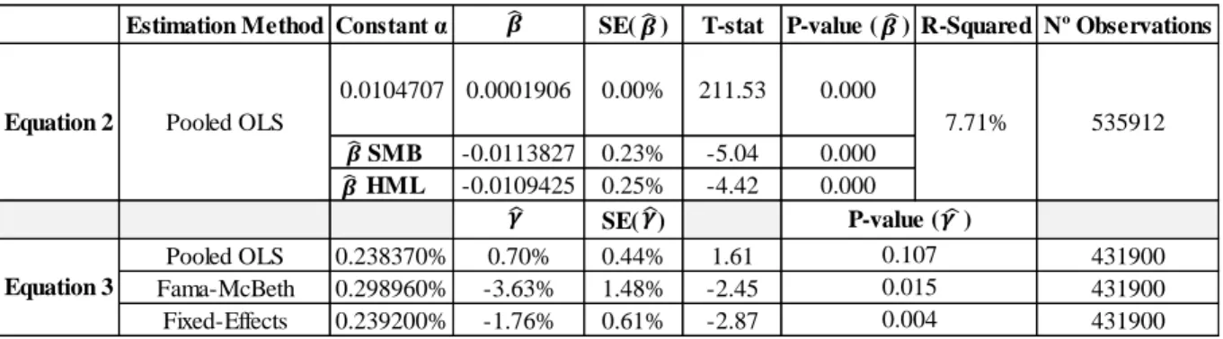
Table 1.1 Regression output (estimated results for 1st and 2nd stages) with idiosyncratic effect
Estimation Method Constant α SE( ) T-stat P-value ( ) R-Squared Nº Observations
SE( ) Pooled OLS 0.238390% 0.66% 0.44% 1.52 431900 Fama-McBeth 0.299440% -3.63% 1.48% -2.45 431900 Fixed-Effects 0.239220% -1.84% 0.61% -2.99 431900 P-value ( ) 0.128 0.015 0.003 Pooled OLS 0.0104009 535912 Equation 3 0.0001905 0.00% 211.51 0.000 7.70% Equation 1
13
Table 1.2 Regression output with factors (estimated results 1st and 2nd stages) with idiosyncratic effect
These results come to confirm the view explored by Engelberg, Reed and Ringgenberg (2012) that suggests the ability of short sales to predict future returns due to their information processing capacity after public release. This shows that the information is related to the firm.
The results in tables 1.1 and 1.2 corroborate the view that there is a propensity for short-sellers to target particular firms, as such their ability to process information is not merely market-wide but also firm-specific. According to Engelberg, Reed and Ringgenberg (2012) the ability of short-sales to predict future returns is particularly strong for non-market making trades.
The firm-specific residuals from Pooled OLS regressed above in Equation 3 have more significant results under Fama-McBeth and Fixed-Effects indicating that specific firms appear to trigger short-sellers’ interest due to their specific characteristics. For instance Anderson, Reeb and Zhao (2012) suggest that informed trading appears to drive a greater level of short sales in family firms than in nonfamily firms. As family firms’ characteristics and short-sales seem to contain useful information in predicting stock returns.
4.1.2 Fixed-Effects
The use of Fixed-Effects’ models allows us to decompose the disturbance term into an individual specific effect 𝜇𝑖 and idiosyncratic variable which capture the remainder disturbance term 𝑣𝑖,𝑡 (Brooks 2002). Therefore, Fixed-Effects enable to distinguish the firm-specific short
Estimation Method Constant α SE( ) T-stat P-value ( ) R-Squared Nº Observations
SMB -0.0113827 0.23% -5.04 0.000 HML -0.0109425 0.25% -4.42 0.000 SE( ) Pooled OLS 0.238370% 0.70% 0.44% 1.61 431900 Fama-McBeth 0.298960% -3.63% 1.48% -2.45 431900 Fixed-Effects 0.239200% -1.76% 0.61% -2.87 431900 Equation 3 7.71% 535912
Equation 2 Pooled OLS
0.0104707 0.0001906 0.00% 211.53 0.000 P-value ( ) 0.004 0.107 0.015
14
interest from the aggregate market shorting, net of the average short interest level associated with the stock:
𝑆𝐼𝑅𝑖𝑡 = 𝛽0+ 𝛽1𝑇𝑜𝑡𝑆𝐼𝑅𝑡+ 𝜇𝑖 + 𝑣𝑖,𝑡 (5) 𝑆𝐼𝑅𝑖𝑡 = 𝛽0+ 𝛽1𝑇𝑜𝑡𝑆𝐼𝑅𝑡+ 𝛽2𝑆𝑀𝐵𝑡+ 𝛽3𝐻𝑀𝐿𝑡+ 𝜇𝑖 + 𝑣𝑖,𝑡 (6)
The estimation of Equations (5) and (6) consist in regressing the short interest ratio 𝑆𝐼𝑅𝑖𝑡 against the aggregate market shorting (systematic shorting) 𝑇𝑜𝑡𝑆𝐼𝑅𝑡. The first-step estimation with the Fixed-Effects’ method leads to the overall R-squared of 7.70% for Equation (5) and 7.71% for Equation (6). The p-values of both equations are close to zero for the global joint significance, that leads to the conclusion the models have a good explanatory power.
The results can be find in tables 2.1 and 2.2
Table 2.1 Regression output (estimated results for 1st and 2nd stages) with idiosyncratic effect
Table 2.2 Regression output with factors (estimated results 1st and 2nd stages) with idiosyncratic effect
The statistical significance of the idiosyncratic component in Equation (3) have demonstrated homogeneous results across the whole estimations with 𝛾 ∈ [-4.08%; -1.50%]. 1 Hence if the idiosyncratic variable increases 1 unit, estimated returns over the next month will decrease on average in the range [-4.08%; -1.50%] ceteris paribus.
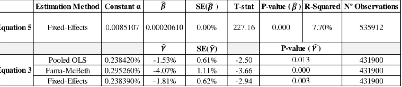
Estimation Method Constant α SE( ) T-stat P-value ( ) R-Squared Nº Observations
SE( ) Pooled OLS 0.238420% -1.53% 0.61% -2.50 431900 Fama-McBeth 0.295260% -4.07% 1.11% -3.66 431900 Fixed-Effects 0.238390% -1.81% 0.62% -2.94 431900 P-value ( ) 0.013 0.000 0.003 Equation 5 Fixed-Effects 0.0085107 0.00020610 0.00% 227.16 0.000 Equation 3 7.70% 535912
Estimation Method Constant α SE( ) T-stat P-value ( ) R-Squared Nº Observations
SMB -0.0073610 0.16% -4.56 0.000 HML -0.0047686 0.18% -2.70 0.007 SE( ) Pooled OLS 0.238420% -1.50% 0.61% -2.45 431900 Fama-McBeth 0.295110% -4.08% 1.11% -3.66 431900 Fixed-Effects 0.238390% -1.79% 0.62% -2.90 431900 Equation 3 7.71% 535912 0.00% 226.36 0.000 Equation 6 Fixed-Effects 0.0088588 0.0002058 P-value ( ) 0.014 0.000 0.000
15
The consistent negative signs obtained both with Pooled OLS and Fixed-Effects indicate the idiosyncratic variable of the previous period to have a consistent trend in driving down returns at the current time t. Jiao, Massa and Zhang (2016) suggest that persistent performance is likely to be associated with superior firm-specific information than other information sources, reflecting superior managerial skill in information processing.
The individual significance of the idiosyncratic variable has also been strongly significant throughout the different estimation’s methods, and the observed p-values close to zero illustrate the significance of that variable.
It should be noted that once again under the Fama-McBeth approach coefficients yield the lowest values in comparison to other methods, Equation (3) predicts an impact on returns of -4.07% (without factors) and -4.08% (with factors).
Huszár, Tan and Zhang (2016), found that short-sellers exploit industry information in conjunction with firm information in their trading strategies. The presented findings with Fixed-Effects corroborate these same conclusions, either with or without dynamic factors, however when these are to be included coeffients become less negative on Pooled OLS and Fixed-Effects estimations, despite the small differences one can say that size and value factors on the long-short Portfolios do capture information that is contained in the idiosyncratic component.
As suggested by Huszár, Tan and Zhang (2016) short-sellers focus on heterogeneous industries with greater information complexity, where they can exploit private information or gain from superior information-processing skills. In this sense dynamic portfolio factors help to “filter” information that is not firm-specific, suggesting short-sellers do not restrict their trading behaviour to factor investing.
Long-short Portfolio strategies small-minus-big and high-minus-low consist in going long on small-cap firms and shorting large caps 𝑆𝑀𝐵𝑡, while 𝐻𝑀𝐿𝑡 seeks the value premium by going long on value stocks and shorting growth firms (Ang 2014), both factors have negative
16
coefficients meaning a unit increase in each strategy leads to a decrease in 𝑆𝐼𝑅𝑖,𝑡 Anderson, Reeb and Zhao (2012) found firm size to be negatively related to abnormal short sales and family firms to experience greater abnormal short sales prior to negative earnings surprises.
4.2 Systematic effect over returns
4.2.1 Pooled OLS
Estimated Equations (1) and (4), (2) and (4) in a way challenge the findings above, the results show that 𝛼̂ ∈ [-13.12%; -4.72%] and p-values are close to zero. In tables 4.1 and 4.2 1 we can see that the overall market shorting do decrease returns on average -12.71% (without factors) and -13.12% (with factors) ceteris paribus by Pooled OLS. Estimations in tables 4.1 and 4.2 (Equation 4), Fixed-Effects results only present significant coefficients when factors were introduced, while the Fama-McBeth estimations are not significant with or without factors, as a consequence these results will be neglected.
Table 4.1 Regression Output by Pooled OLS (estimated results 1st and 2nd stages) with systematic effect
Table 4.2 Regression output by Pooled OLS and factors (estimated results 1st and 2nd stages) with systematic effect
Estimation Method Constant α SE( ) T-stat P-value ( ) R-Squared Nº Observations
SE( ) Pooled OLS 0.0066026 -12.71% 1.45% -8.75 431900 Fama-McBeth -0.0042113 14.56% 11.4% 1.28 535911 Fixed-Effects 0.003693 -3.94% 2.02% -1.95 431900 P-value ( ) 0.000 0.201 0.052
Equation 1 Pooled OLS 0.0104009 0.0001905 0.00% 211.51 0.000 7.70% 535912
Equation 4
Estimation Method Constant α SE( ) T-stat P-value ( ) R-Squared Nº Observations
SMB -0.0113827 0.23% -5.04 0.000 HML -0.0109425 0.25% -4.42 0.000 SE( ) Pooled OLS 0.673800% -13.12% 1.45% -9.03 431900 Fama-McBeth -0.372590% 12.28% 11.27% 1.09 535911 Fixed-Effects 0.395060% -4.72% 2.02% -2.34 431900
Equation 2 Pooled OLS
0.0104707 0.0001906 0.00% 211.53 0.000 7.71% 535912 P-value ( ) 0.000 0.278 0.019 Equation 4
17
Our evidence suggests that an increase in systematic market shorting leads to a negative impact on stock returns, this is somehow consistent with the findings of Boehmer, Jones and Zhang, (2007) that concluded shorts are informed regardless of the account type of trading, institutional, member-firm proprietary and non-program institutional shorts. Despite some acting as market-makers they possess important information that has not yet been incorporated in the price of stocks.
The significant impact on returns of -12.71% and -13.12% has to be analysed at the aggregate level, therefore it is considered that such impact corresponds to the overall market. Such results could be the reflection of market-wide mispricing in contrast to firm-specific information. Lynch, et al. (2013) concluded that markets aggregate information and impound it into prices, due to relevant macroeconomic information from news announcements, finding negative relationships between lagged aggregate selling and macroeconomic news and that short-sellers have superior information at the aggregate market level.
4.2.2 Fixed-Effects
As mentioned in section 4.1.3, Fixed-Effects allow us to decompose the disturbance term into an individual specific effect. That is what is considered in the results below but within the systematic shorting framework.
The results obtained with Fixed-Effects are fairly identical to the Pooled OLS regarding the estimated coefficients, as well as the Fama-McBeth was neglected by not being statistically significant, as shown in tables 5.1 and 5.2 regression output results.
18
Table 5.1 Regression output by Fixed-Effects (estimated results 1st and 2nd stages) with systematic effect
Table 5.2 Regression output by Fixed-Effects and factors (estimated results 1st and 2nd stages) with systematic effect
It is observed on tables 5.1 and 5.2 that 𝛼̂ ∈ [-11.89%; -3.64%] and p-values are close to 1 zero. In line with the Pooled OLS estimations, Equation 4 estimated by Pooled OLS yields the lowest results of, -11.75% (without factors) and -11.89% (with factors).
Fixed-Effects estimations in Equation 4, as in the previous findings, only have significant coefficients when factors were introduced. Despite the similarities of the results, overall, systematic short-selling under Fixed-Effects shows a lower impact on returns in comparison to Pooled OLS.
When we talk about systematic short-selling it is important to acknowledge that although trades may not be exclusively firm-specific, they can also be in fact determined by particular timeframes or specific timings that influence the decision (or not) to trade.
The amount of systematic shorting once it is executed at the market level is economically larger than idiosyncratic shorting, as such we observe larger magnitudes of the coefficients.
Estimation Method Constant α SE( ) T-stat P-value ( ) R-Squared Nº Observations
SE( ) Pooled OLS 0.0062804 -11.75% 1.34% -8.75 431900 Fama-McBeth -0.0038422 13.46% 10.51% 1.28 535911 Fixed-Effects 0.0035931 -3.64% 1.87% -1.95 431900 227.16 0.000 7.70% P-value ( ) 0.000 0.201 0.052 535912 Equation 4 Equation 5 Fixed-Effects 0.0085107 0.00020610 0.00%
Estimation Method Constant α SE( ) T-stat P-value ( ) R-Squared Nº Observations
SMB -0.0074 0.16% -4.56 0.000 HML -0.0048 0.18% -2.7 0.007 SE( ) Pooled OLS 0.632730% -11.89% 1.35% -8.84 431900 Fama-McBeth -0.0035591 11.96% 10.6% 1.13 535911 Fixed-Effects 0.366830% -3.87% 1.87% -2.07 431900 Equation 3 Equation 6 Fixed-Effects 0.0088588 0.00021 0.00% 225.58 0.000 7.71% 535912 P-value ( ) 0.000 0.260 0.039
19
However, the lower quality of information in these shorts reflects a higher risk, the systematic market risk that cannot be eliminated using firm-specific information.
4.3 Analysis of Residuals
In Table 6 we have the summary statistics for the residuals from estimated Equations (1-2) and Equations (5-6).
The residuals of Pooled OLS and Fixed-Effects’ methods illustrate identic estimated moments, nonetheless should be noted that when we take into consideration firms’ heterogeneity (Fixed-Effects) we observe smaller means and lower standard deviations, that is the result of the firm-specific shorting as firms’ characteristics are taken into account.
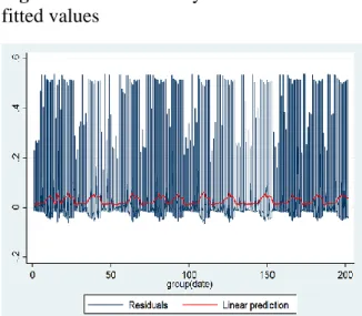
Figure 1. Residuals by Pooled OLS and Figure 2. Residuals by Pooled OLS and
fitted values fitted values with Factors
Figure 3. Residuals by Fixed-Effects and Figure 4. Residuals by Fixed-Effects and
fitted values fitted values with Factors
20
Looking at Figures (1-2) to (3-4) and Table 6, we observe that across all estimation methods residuals (idiosyncratic component) have a higher range in comparison to the predicted values, overall the variance of residuals seems constant over time.
The range in which firm-specific information varies is fairly larger than the systematic one, another important aspect is that predicted values are always positive (Figures 1 to 4 and Table 6), while residuals are positive and negative, particularly negative when estimated by Fixed-Effects.
The positive pattern of predicted values somehow shows the consistent amount of shorting that occurs at the systematic level. On the other hand, the residuals that illustrate the firm-specific shorts, have negative amount of shorting. Under Fixed-Effects that incorporate the firm’s heterogeneity we see negative shorting, that is explained by increased short-selling in periods of negative news that is offset by the absence of short-selling in good news’ periods, however systematic shorting continues to take place regardless of the information framework leading to negative firm-specific shorts.
Table 6. Summary statistics of the estimated residuals and predicted values
4.4.1 Information flow
The findings with Pooled OLS and Fixed-Effects on systematic shorting are somehow striking if we are to believe short-sellers trade on firm-specific information, regardless of what
Estimation methods Obs Mean Stdev. Min Max
Pooled OLS 535912 3.33E-12 0.049704 -0.0652 0.54170
Pooled OLS with Factors 535912 -6.05E-12 0.049703 -0.0645 0.54153 Fixed-Effects 535912 1.30E-12 0.034952 -0.3941 0.54468 Fixed-Effects with Factors 535912 1.63E-12 0.034952 -0.3941 0.54457 Pooled OLS 535912 0.033456 0.014361 0.01318 0.06523 Pooled OLS with Factors 535912 0.033456 0.014366 0.01205 0.06451 Fixed-Effects 535912 0.033456 0.015538 0.01151 0.06784 Fixed-Effects with Factors 535912 0.033456 0.015517 0.01103 0.06740 ,
21
shorts are more informative these results have to be accounted as having a considerable degree of validity.
The information in tables 4.1-4.2 and 5.1-5.2, the magnitude of the coefficients indicates that systematic shorting somehow predict returns, the predictions may be or not informed. As suggested by Blau and Wade (2011), preferred clients may be tipped or sophisticated investors were able to acquire information in some other way. On the other hand they concluded short-selling prior to analyst recommendations to be motivated by speculation than by information.
The nature of the information that drives systematic shorting is more ambiguous than firm-specific, for such reason these results incorporate a diversity of information that can hardly be distinguished. Comerton-Forde, et al. (2015) agree that given the variety and breath of information sources, short-sellers are heterogeneous in terms of the nature of their information and investment timeframes.
Overall the influence of systematic shorting upon returns seems to be a combination of momentary information acquisition (opportunistic arbitrages) and pure speculative hedging behaviour that due to the frequency of trading exercised, in a way has an impact on stock returns.
4.4.2 Information clustering
There is evidence the informativeness of the shorts to be clustered, it is possible to identify when and where informed short-selling takes place. The levels of information vary across space and time, enabling to distinguish between systematic and idiosyncratic shorting.
According to Blau, Ness and Ness (2010) more short-selling occurs in the NYSE however Nasdaq short-selling is more informed, this suggests shorting in the NYSE to be more systematic and less informed while the Nasdaq with fewer short trades yield higher predictability.
22
It is also important to acknowledge that the time span during which short-selling mostly occurs, is relevant in order to explain the flow of information. Alldredge, Blau and Brough (2012) found that after-hours informed short-selling to contain less return predictability than regular market hours.
Hence market activity is a relevant vehicle through which information flows and from which informed short-sellers capture information, as such, idiosyncratic shorting is subject to the market dynamics and not only private information.
V. Conclusion
Throughout this paper a clear distinction was made between systematic and idiosyncratic short-selling, being the first commonly believed as a less informed way of trading and the latter a more informed and firm-specific trading approach.
It was attempted to identify which kind of impact both types of shorting have on stock returns, in that way this work tried to illustrate the degree to which short-selling can in fact predict future stock returns and which type (systematic or idiosyncratic) is better at doing it.
It was concluded that systematic shorting has a larger negative impact on returns than idiosyncratic shorting, however we find that the idiosyncratic component yields more consistent results than the systematic one, firm-specific frequent smaller declines, while systematic less frequent larger declines. As a result, idiosyncratic short-selling shows evidence of being a better predictor, thus a more reliable information source.
The estimated effects of idiosyncratic component over returns varies in the range of [-4.08%; -1.50%] while the effect of systematic component over next period returns varies in the range of [-13.12%; -3.64%]. Both components are statistically significant to explain the behaviour of log-returns.
Considering that Jiao, Massa and Zhang (2016) suggest that persistent performance is likely to be connected with superior firm-specific information. Throughout the idiosyncratic analysis
23
it is observed that both estimations methods deliver persistent significant negative signs, reflecting superior information processing.
We concluded there are different ways through which information disseminates, information can be firm-specific or mark-wide, markets are capable of gathering information that will be reflected on prices, therefore markets are an important channel of information, for both idiosyncratic and systematic sellers. However the informativeness of systematic short-selling tends to be more limited due to the ambiguity of the sources of information.
The fact there is a clustering of information regarding shorts, research should go deeper in identifying which sectors and industries are perceived as less trustworthy, in particular technology firms’ stocks known for higher volatilities. This would indicate what the market believes to be sustainable as a future trend.
While this paper discriminates the different types of short-selling, we believe it is equally important the understanding of the sectors and industries in which shorting mostly occurs. As future research we suggest a focus on industry analysis in order to provide a better understanding of short-sellers’ behaviour.
24
VI. Bibliography
Alldredge, Dallin M., Benjamin M. Blau, and Tyler J. Brough. 2012. “Short selling after hours.”
Journal of Economics and Business 439-451.
Anderson, Ronald C., David M. Reeb, and Wanli Zhao. 2012. “Familly-Controlled Firms and Informed Trading: Evidence from short sales.” The journal of Finance 351-386. Ang, Andrew. 2014. A Systematic Approach To Factor Investing. New York: Oxfor University
Press.
Asquith, Paul, Parag A. Pathak, and Jay R. Ritter. 2005. “Short interest, institutional ownership and stock returns.” Journal of Financial E conomics 243-276.
Au, Andrea S., John A. Doukas, and Zhan Onayev. 2008. “Daily short interest, idiosyncratic risk and stock returns.” Journal of Financial Markets 290-316.
Best, Roger J., Ronald W. Best, and Jose Mercado-Mendez. 2008. “Do short sellers anticipate large stock price changes?” Academy of Accounting & Financial studies 71-84.
Biggs, Barton M. 1966. “The short interest- A false proverb.” Financial analysts journal 111-116.
Blau, Benjamin M., and Chip Wade. 2011. “Informed or speculative: Short selling analyst recommendations.” Journal of Banking and Finance 14-25.
Blau, Benjamin M., Bonnie F. Van Ness, and Robert A. Van Ness. 2010. “Information in short selling: Comparing Nasdaq and the NYSE.” Review of Financial Economics 1-10. Boehmer, Ekkehart, Charles M. Jones, and Xiaoyan Zhang. 2007. “Which shorts are
informed?” Journal of Finance.
Brent, Averil, Dale Morse, and E. Kay Stice. 1990. “Short interest: Explanations and tests.”
25
Brooks, Chris. 2002. Introductory Econometrics for Finance. Cambridge: Cambridge University Press.
Callen, Jeffrey L., and Xiaohua Fang. 2015. “Short Interest and stock price crash risk.” Journal
of Banking & Finance 181-194.
Chakrabarty, Bidisha, and Andriy Shkilko. 2013. “Information transfers and learning in financial markets: Evidence from short selling around insider sales.” Journal of Banking
& Finance 1560-1572.
Comerton-Forde, Carole, Binh Huu Do, Philip Gray, and Tom Manton. 2015. “Assessing the information content of short-selling metrics using daily.” Journal of Banking and
Finance 188-204.
Dechow, Patricia M., Amy P. Hutton, Lisa Meulbroek, and Richard D. Sloan. 1999. “Short-Sellers, fundamental analysis and stock returns.”
Desai, Hemang, K. Ramesh, S. Ramu Thiagarajan, and Bala V. Balachandran. 2002. “An investigation of the informational role of short interest in the Nasdaq market.” Journal
of finance 2263-87.
Diamond, Douglas W., and Robert E. Verrecchia. 1987. “Constraints on Short-Selling and Asset Price Adjustment to Private Information.” Journal of Financial Economics 277-311.
Diether, Karl B., Kuan-Hui Lee, and Ingrid M. Werner. 2008. “Short-Sale Strategies and Return Predictability.” Society for Financial Studies (Oxford University Press) 575-607. Engelberg, Joseph E., Adam V. Reed, and Matthew C. Ringgenberg. 2012. “How are shorts
informed? Short sellers, and information processing.” Journal of Financial Economics 260-278.
Fama, Eugene F., and James D. MacBeth. 1973. “Risk, Return and Equilibrium.” The Journal
26
Goyal, Amit. 2011. “Empirical cross-sectional asset pricing: a survey.” Swiss society for
Financial Market Research 3-38.
Hurtado-Sanchez, Luis. 1978. “Short interest: Its influence as stabilizer of stock returns.”
Journal of Financial & Quantitative Analysis 965-985.
Huszár, Zsuzsa R., Ruth S.K Tan, and Weina Zhang. 2016. “Do Short Sellers exploit industry information?” Journal of Empirical Finance.
Jiao, Yawen, Massimo Massa, and Hong Zhang. 2016. “Short selling meets hedge fund 13F: An anatomy of informed demand.” Journal of Financial Economics 1-24.
Lynch, Andrew, Biljana Nikolic, Xuemin (Sterling) Yan, and Han Yue. 2013. “Aggregate short selling, commonality and stock returns.” Journal of Financial Markets 199-229. Mohamad, Azar, Aziz Jaafar, Lynn Hodgkinson, and Jo Wells. 2013. "Short Selling and stock
returns: Evidence from the UK." The British Accounting Review (Elsevier) 125-137. Rapach, David E., Matthew C. Ringgenberg, and Guofu Zhou. 2016. “Short Interest and
aggregate stock returns.” Edited by William Schwert. Journal of Financial Economics (Elsevier) 46-65.