A Work Project, presented as part of the requirements for the Award of a Master Degree in
Economics from the NOVA – School of Business and Economics.
THE EFFECTS OF CRISES IN EUROPE:
IMPACT, TWINS AND RECOVERY TIME
SIMON ANDREAS MOSIMANN 33079
A Project carried out on the Master in Economics Program, under the supervision of:
Paulo Manuel Marques Rodrigues
Abstract
The goal of this thesis is to examine the effect of a systemic crisis on GDP growth. The
balanced panel analysis of 16 European countries over the time period 1970 – 2017 shows
that a crisis has severe consequences as growth is reduced by 1.8% for each crisis year. Twin
Crises and complex crises prove to be extraordinarily damaging. After the crisis has ended a
country undergoes on average two years of recovery time until the pre-crisis growth trend is
re-established. The results are highly robust to different control variables, specifications and
datasets.
Keywords
output loss, growth, systemic crisis, recovery
This work used infrastructure and resources funded by Fundação para a Ciência e a Tecnologia
(UID/ECO/00124/2013, UID/ECO/00124/2019 and Social Sciences DataLab, Project 22209),
POR Lisboa (LISBOA-01-0145-FEDER-007722 and Social Sciences DataLab, Project 22209)
1. Introduction
Pictures of people lining up in front of counters of the British bank “Northern Rock” are
in good memory as the subprime crisis spilled over from the US to Europe and the general
public worried that their deposits are not safe anymore. Some years later, on the southern end
of the continent furious demonstrators in Athens were photographed when they rioted in fear
of losing their jobs as a result of the rigorous austerity plan forced upon the country. The two
images are proof of the consequences financial crises can have for the average worker. What
first starts as a hard to grasp phenomena with asset prices decreasing or government bond
spreads increasing can rapidly turn into harsh life changes for many. Total unemployment
among the 27 EU countries rose by 4% in the crisis year 2008 (Eurostat, 2009) and future generations in Greece will have to repay a debt mountain of €322 billion over the next 42 years
(Baynes, 2018).
The two incidents have different origins as one was caused by disruptions in the banking
sector and the other by extensive sovereign debt, but similar negative consequences for the real
sector as both times production plunged and a recession unfolded. The present master thesis
attempts to investigate whether these two extreme events are exceptional outliers or if financial
crises have significant effects on economic output. Furthermore, it will be evaluated if complex
crises and so-called twin crises, events where two different crisis types happen at the same time,
have particularly harmful consequences. The third question tackled in this paper is whether a
country experiences a recovery time after the end of a crisis and if it does so, how many years
it takes for the economy to reach the pre-crisis growth level. To find answers to these three
inquiries, a newly published systemic crisis database by the ECB and data from 16 European
countries over the time span of nearly 50 years will be used for a balanced panel analysis with
country fixed effects.
Section 2 is dedicated to an overview of existing research in the field of financial crisis’
financial crisis definition, statistical models, causality issues and different crisis causes. In the
next section the data used is described with a detailed look at the features of the ECB’s crisis
database, followed by a section explaining the characteristics of the different crisis types listed
in the database. Section 5 presents the methodology together with the model specification and
several diagnostics test. The performed analysis is based on a balanced panel with country fixed
effects and Driscoll-Kraay standard errors (Driscoll and Kraay, 1998). The main results of this
paper are presented in the 6th section. A significant negative effect of a systemic crisis on GDP
growth is found with a decline of 1.8% per crisis year. Alongside with the results come potential
explanations of the reasons responsible for the reduction of the growth rate. This section
finishes with a series of robustness checks in order to evaluate if the findings hold in different
model environments such as a bigger set of control variables or excluding the global financial
crisis. Within the robustness checks also an analysis incorporating all 28 EU states plus Norway
for the shorter period of 1995 – 2017 can be found. For this alternative dataset the negative
impact of a systemic crisis with an estimated 2.4% per crisis year seems to be considerably
larger than in the core dataset.
In section 7 an analysis is performed to examine the impact of different crisis types. Three
combinations of twin crisis as well as complex crises seem to have a significant marginal effect
on output that goes beyond the simple addition of the components. The penultimate section
focuses on the crisis recovery. The growth IRF, calculated with the local projection method,
reveals that on average a country reaches its normal growth trend two years after the crisis has
ended. The last section sums up all results and gives future research recommendations.
2. Literature Review
There exists a broad field of research evaluating the effects of financial crises on
economies. One group of studies focuses especially on long time periods, which can extend up
to 200 years. Among this group is the work of Reinhart and Rogoff (2014), Bordo, Eichengreen,
influential book This Time is Different Reinhart and Rogoff (2009) defined a detailed dataset
of financial crises starting in the year 1800. Using this dataset, the authors evaluated the impact
on GDP by looking at 100 systemic crises. To quantify the effect the peak-to-trough fall is used,
which is the difference in real GDP per capita between the start of the crisis and the bottom of
the downturn. The authors use simple summary statistics and report that average peak-to-trough
fall was 11.5% and average peak-to-recovery time was 8.3 years (Reinhart and Rogoff, 2014).
Bordo et al. (2001) conduct a regression analysis with observations from 1880 to 1997 and
conclude that following a crisis a country on average experiences a downturn of 2 to 3 years
connected to an overall output loss of 5 – 10% of GDP. But in general, research papers on
financial crises focus on shorter periods, usually not more than the past 50 years.
One crucial point among the different studies is the used definition for financial crises and
the according start and end dates of the crises. One group of researchers use crisis databases that can be considered as ‘standard’ databases. Usually this is either Reinhart and Rogoff (2009)
or Laeven and Valencia (2008, 2013) and before 2008 it was Caprio and Klingebiel (1996) or
Demirgüç-Kunt and Detragiache (1998). Another group of papers use the mentioned ‘standard’
databases but combine them with each other or add own amendments, as Hutchinson and Noy
(2005) did. They simply combine Caprio and Klingbiel (1996) and Demirgüç-Kunt and
Detragiache (1998) by defining a crisis if it is mentioned in either of the two databases. A third
group of authors come up with their own, sometimes exotic calculations for systemic crises.
Romer and Romer (2015) focus on disruptions of the credit supply and classify a financial crisis
on a scale from 0 to 15, with 7 being a moderate crisis. This is a new approach as all the other
mentioned databases work with a binary definition where a country either is in a crisis or not.
The lack of a universal definition for systemic crises leads to difficulties in comparing the
outcomes of studies with each other, as often different definitions were used. The differences
in definitions have a not negligible effect on the results. The ECB recognized this problem and
events to support the calibration of models in macroprudential analysis and policy (ECB, 2017).
This paper will for the first time use this newly published dataset as part of a panel analysis to
estimate the general impact of a crisis on output.
Panel analysis is a common statistical tool used to quantify the impact of systemic crises.
It is used in the work of Furceri and Zdzienicka (2011), Dell’Ariccia, Detragiache and Raja
(2005), Teulings and Zubanov (2014) as well as Oulton and Sebastiá-Barriel (2017). An
unbalanced panel of 154 countries from 1970 – 2008 is used by Furceri and Zdzienicka (2011)
to analyse debt crises. They use several control variables that are believed to influence growth
to single out the true effect of a crisis. Furthermore, the two-step GMM-system estimator is
used to address problems of endogeneity. Their analysis suggests that if a country is in a debt
crisis the contemporaneous output is lowered by 5.5% on average. Oulton and Sebastiá-Barriel
(2017) use fixed effects panel regressions, which are estimated by the Arellano-Bond (Arellano
and Bond, 1991) method and not by the common least squares regression method as the former
is able to deal with the issue of lagged dependent variables not being exogenous. The authors
find that a banking crisis decreases GDP per capita by 1.8% for every crisis year. In addition to
the panel analysis, impulse response functions (IRF) are used to illustrate the response of output
to a financial crisis. The IRFs are generated with the local projection method developed by
Jordá (2005). Teulings and Zubanov (2014) slightly change the method suggested by Jordá and
show with their IRFs that 7 years after the start of a crisis the loss of GDP reaches its maximum.
For the present thesis data from 16 countries over 48 years will be analysed with a fixed effects
model specification. An IRF based on the local projection method will be used to compute the
response of growth to a crisis.
Another crucial point in the analysis of financial crises is the question of causality. Just
because GDP growth decreases in times of financial crises does not directly imply that the
decline was caused by the crisis. It could be possible that a third unknown factor is responsible
sector and at the same time negatively affect aggregate demand, what in this case would lead
to the conclusion that financial crises and GDP growth are independent of each other. To
investigate if banking crises have an impact on economic output Dell’Ariccia et al. (2005)
analysed if industries more dependent on bank loans suffer relatively more during a banking
crisis. The results show that financially dependent sectors lose about 1 percentage point of
performance in each crisis year compared to sectors less dependent on banks. Thus, the authors
conclude that a financial crisis has real effects on industries. The direction of the causality has
to be tested too, as it could be possible that declining growth causes a crisis and not vice versa.
Jordà et al. (2013) approach this issue by comparing recessions accompanied by a financial
crisis to normal recessions. By looking at data from 14 countries during 1870 to 2008 they find
that a recession accompanied by a crisis is significantly much longer and more painful than a
regular downward business cycle. Similar results are revealed by Bordo et al. (2001) using the
same method of comparing the two types of recessions. These findings let assume that crises
are at least partly responsible for the occurring economic slowdown. In order to not overload
this paper, causality will not be questioned. It will be assumed that the results obtained by the
mentioned scholars hold true for the analysed countries and time period.
Not every crisis has the same characteristics. Some are solely caused by disruptions in one
area whereas others have multiple origins like a simultaneous banking and currency crisis. The
latter were studied by Hutchison and Noy (2005) who compared the so-called “twin crises” to
crisis events when only the banking sector or the exchange rate were troubled. The outcomes
of their work show that single currency and banking crises reduce growth by 5%-8% and
8-10% respectively over 2-4 years crisis duration. However, the effects of twin crises do not
exceed the pure additional negative impact of the two crises and thus the assumption that twin
crises have amplifying dynamics is neglected. On the contrary Furceri and Zdzienicka (2011)
pure addition of the two effects. Section 7 is dedicated to the thorough analysis of the research
question if the different crisis types change the impact on output.
In summary, existing research has shown a very robust negative impact of financial crises
on GDP. The estimates range from around 1.5% up to 6% loss of GDP growth for each crisis
year. Furthermore, proofs were found for the financial crises independent direct impact on the
real sector. The declines of economic output could not be fully explained by normal business
cycles or other third factors. When it comes to multiple origin crises there exists mixed evidence
whether twin events are worse than the added effects of their components or not.
3. Data
The used dataset consists of GDP data, the systemic crisis database and the control
variables. The values for real GDP are obtained from the World Bank and are measured in
constant 2010 bn US$. The start and end dates for systemic crises are taken from the ECB/ESRB
EU crises database (ECB 2017), where crises were identified in a two-step approach. First, a purely analytical analysis using a financial stress index, which takes price changes in key
financial market segments into account, resulted in a list of events of high financial distress. In
the second step the list got revised by the National Authorities who now relied on qualitative
information. An event got flagged as a systemic crisis if at least one of the following criteria
was fulfilled: (1) The supply of credit to the non-financial sector shrinks what contributes to
substantially negative economic outcomes, (2) financial market infrastructure is dysfunctional
and/or there are bankruptcies among large banks, (3) policies were adopted to preserve financial
stability (ECB, 2017). Furthermore, the revising National Authorities could add events to the
systemic crises list that were not detected by the financial stress index but fulfilled the criteria.
Apart from the systemic crises the ECB dataset lists 43 residual events, which are periods
of elevated financial distress but were not considered to be a systemic crisis. In the final dataset
50 systemic crises were detected among the 28 EU countries and Norway during 1970 – 2017.
used among scholars studying financial crises, the most obvious difference is that the LV
database only allows a crisis to have one origin (banking, currency or sovereign debt) whereas
the ECB works with non-exclusive categories. This results in the allowance of complex crises
with multiple origins. Depending on what risk materialised, the event in the ECB database is
labelled with one or multiple types from the following set of options: (1) banking risk, (2)
significant asset price correction, (3) sovereign debt risk, (4) currency risk or (5) transition. In
some incidents a complex event in the ECB dataset covers multiple different events listed by
Laeven and Valencia. Overall a total of 30 events can be found in both datasets, whereas the
ECB list contains 16 events not listed by Laeven and Valencia and the LV list contains 1 event
that the ECB did not consider as a systemic crisis. Therefore, the ECB seemed to apply less
strict requirements to label an event as a systemic crisis compared to the criteria used in the LV
list. GDP data was not available for all countries during the period 1970 - 2017, why the sample
for the analysis was reduced to 16 countries in order to ensure a balanced panel. The analysed
economies experienced a total of 27 systemic crises lasting on average 4.6 years. The crisis
dates are listed with monthly data whereas the dataset used for this thesis deals with yearly data.
Therefore, a country is considered to be in a crisis if it experienced 6 or more months of crisis
in the respective year.
Three control variables were selected to account for influences on economic output other
than systemic crises. In accordance with the expenditure approach of the GDP, the variables
private household consumption, general government expenditure and domestic investment are
included. The net exports are excluded as they showed no significant effect on GDP growth in
the used dataset. All control variables are expressed as % of GDP and are obtained from the
World Bank. More information on the data can be found in Appendix B.
4. Characteristics of Different Crisis Origins
The following section explains the characteristics of the different crisis types mentioned
the risks that materialise during a crisis. These are: sovereign risk, banking risk, currency risk,
significant asset price correction and transition. The last category will not be analysed further
in this paper, as the circumstances in these events are caused by the fall of the Soviet Union and
are thus considered to be rather unique and not relevant for macroprudential analysis.
Sovereign risk relates to situations when a government faces difficulties to obtain enough funding for due payments which can result in a sovereign default. Even though sovereign
defaults nowadays are more associated with emerging markets, major European countries have
a long history of external defaults. Prior to 1900 Spain defaulted no fewer than 13 times
followed by France with a total of eight defaults (Reinhart and Rogoff, 2009), what shows that
these rich countries went through similar difficulties in their emerging phase as countries do
today. Although France and Spain were not in danger of a default recently, there is one famous
case within the sample covered in this paper. Greece, who was struggling with the consequences
of the U.S. subprime crisis, had to admit in October 2009 that it has been manipulating national
accounting by understating deficit figures for years. This cumulated in the loss of confidence
among international investors and the country was cut-off from borrowing at financial markets.
In the spring of 2010 a default seemed unavoidable, which would have possibly triggered bigger
financial turbulences than the collapse of Lehman Brothers did. Several last-minute interventions from the EU, eventually summing up to a total amount of over €240 billion, saved
Greece from declaring bankruptcy (The New York Times, 2016).
Banking risk covers disruptions in the banking sector due to banks either declaring bankruptcy or having severe financing difficulties. The risk mainly arises from the leveraged
position of financial institutions. Banks borrow from the public in form of short-term deposits
that can be redeemed at any time while on the other side of the balance sheets loans are given
out with a long-run repayment schedule. When the public for any reason loses confidence in
the ability of the bank to repay its obligations, the people rush to the counters in order to get
bank assets are in long-term securities, the bank even in the case of having enough funds is not
able to meet the wishes of the panicking depositors and therefore has to declare bankruptcy. In
the end the fear among the depositors results in a self-fulfilling prophecy. In September 2007
worried depositors formed long lines in front of the bank branches of Northern Rock, as they were not satisfied with the British government’s partial insurance plan and wanted to empty
their banking accounts (Reinhart and Rogoff, 2009). The troubles intensified and the British
government had no other choice than to bail out the bank and completely back its liabilities.
Although traditional bank runs do not happen often anymore due to deposit insurances, lost
confidence in the banks ability to repay obligations is still an issue as the interbank lending
dropped drastically during the global financial crisis. Other potential sources for banking risk
are sharply falling asset prices or the default of an important debtor like a big company or an
entire country.
The category currency risk is set up to capture events of speculators challenging the fixed
exchange rate of a country in belief that the government lacks enough resources to back the
peg. Krugman (2007) pointed out that currency crises usually have their origins in a
governments disability to implement fiscal and monetary policies aligned with protecting the
fixed exchange rate. This was one of the criticisms of the 1979 introduced Exchange Rate
Mechanism (ERM) and partly caused the increasing attacks on the weak currencies within the
ERM. On 16 September 1992, what was later named the events of the “Black Wednesday”, the
British government was forced to exit the ERM and give up the fixed exchange rate of the
pound. One day later Italy followed by giving up the peg on the lira. The connected currency
crisis is believed to have intensified the recession in both countries in the early 90s (Fratianni
& Artis, 1996).
Crises categorized within asset price correction suffered under the sudden fall of prices
in one asset class. Usually there was an external cause that had an impact on the domestic stock
Finland to decrease by over 70% within 2 years (ECB, 2017). Oil price shocks in the 70s and
80s are another example for asset price corrections.
5. Methodology
Following previous work in this field, a panel analysis will be conducted that tests
contemporaneous output versus a crisis dummy that takes the value 0 or 1. A set of control
variables influencing economic growth is included in order to single out the true effect of a
systemic crisis and to mitigate the omitted variable bias of time variant effects. The
specification of the empirical model for the panel analysis is,
𝑦𝑖𝑡 = 𝛼𝑖+ 𝛽𝐶𝑖𝑡+ 𝜃′𝑋𝑖𝑡 + 𝜀𝑖,𝑡 (1)
where 𝑦𝑖𝑡 is the annual growth of real GDP for country 𝑖 in year 𝑡. Country-specific effects are
captured in 𝛼𝑖. Economic growth can be influenced by weather conditions, like severe winters
in Finland or dry summers in Spain. Influences like these, who are different from country to
country, but do not change much over time, can be controlled with the country-specific effects. 𝐶𝑖𝑡 is a dummy variable and indicates if country 𝑖 was in a systemic crisis in year 𝑡. 𝑋𝑖𝑡
represents the control variables described in section 3.
The decision to use a fixed effects model specification was made after a series of tests. First
an F-Test confirmed that fixed effects can be found in the panel dataset and therefore a pooled
OLS specification would be less accurate. The Breusch-Pagan LM test also confirmed the
existence of heterogeneity in the considered data. As is common in panel analysis, a Hausman
test was performed to choose between fixed and random effects. A p-value of <0.01 strongly
suggests the use of a model with fixed effects. To check for non-constant variance in the country
population, the modified Wald test for groupwise heteroskedasticity is performed which clearly
indicates heteroskedastic disturbances. Furthermore, the Wooldridge test for autocorrelation
revealed evidence for first-order autocorrelation in the data and the Breusch-Pagan LM test for
independence pointed out the problem of cross-sectional dependence. Because the present data
Driscoll-Kraay standard errors were used to account for these features and therefore reduce the
risk to obtain biased results. All variables used are (trend) stationary at a 10% significance level
according to the Im–Pesaran–Shin unit root test who allows to deal with heterogenous and serial
correlated data. The trend option was used for government consumption, as a time trend is
visible when looking at the corresponding graphs of all countries. Further information on the
model diagnostic tests can be found in Appendix B.
In a second step it will be evaluated if there are different effects by the various crisis types
defined in the dataset. The marginal effect of a crisis type will be estimated by looking at all
crises where the risk type materialised either alone or as part of a twin crisis, together with all
the other crisis types. Equation 2 shows the altered specification
𝑦𝑖,𝑡= 𝛼𝑖+ 𝛽1𝐶𝑖,𝑡𝐵 + 𝛽2𝐶𝑖,𝑡𝐵𝐶𝑖,𝑡𝐴 + 𝛽3𝐶𝑖,𝑡𝐵𝐶𝑖,𝑡𝐶 + 𝛽4𝐶𝑖,𝑡𝐵𝐶𝑖,𝑡𝐷 + 𝛽5𝐶𝑖,𝑡𝐴 + 𝛽6𝐶𝑖,𝑡𝐴𝐶𝑖,𝑡𝐶 (2)
+𝛽7𝐶𝑖,𝑡𝐴𝐶𝑖,𝑡𝐷 + 𝛽8𝐶𝑖,𝑡𝐶 + 𝛽9𝐶𝑖,𝑡𝐶𝐶𝑖,𝑡𝐷 + 𝛽10𝐶𝑖,𝑡𝐷 + 𝛽11𝐶𝑖,𝑡𝑀+ 𝜃′𝑋𝑖𝑡+ 𝜀𝑖,𝑡
where 𝛽1 reflects the effect of a crisis where only banking risk materialised, 𝛽2 to 𝛽4 reflect the
effects of a twin crises where banking risk (B) was one component together with either asset price correction (A), currency risk (C) or sovereign debt risk (D). 𝛽11 captures the effects of all
multiple crises with 3 or more risk components. If 𝛽3 turns out to be significant, the
interpretation is that a banking-currency twin crisis has an additional amplifying effect, that is
different from the effects of a sole banking crisis and currency crisis taken together. In this
second part, data from both systemic crises and residual events were used, as a big majority of
the systemic crises fall under the category of multiple crises. Therefore, an analysis only of the
systemic crises would most likely not render any results regarding the different crisis origins.
6. Results
The baseline model shows that a systemic crisis has a highly significant negative effect on
GDP. If a country suffered from a systemic crisis the GDP will be on average 1.8% lower in
this year compared to the expected trend without any crises (Table 1 Column I). This has
average 4.6 years. A reduction of growth by 1.8% per crisis year usually has far-reaching
consequences since crucial elements of the domestic economy can be affected by the crisis.
If the banking sector predominantly is affected by the crisis, the core intermediation
function of the banks is disrupted as the financial institutions have to cut back in lending
temporarily until calmer waters are reached. This specially harms households and small and
medium enterprises as banks are usually the only source to obtain funding. Big corporations are
more flexible due to the broader set of options like the issue of corporate bonds. Nevertheless,
big firms obviously also suffer under the unfavourable macroeconomic conditions. When the
crisis roots are found in sovereign debt and currency disruptions, one of the damage factors is
the loss of international confidence. The access to external capital markets is denied and foreign
investment drops drastically. Furthermore, external saviours like the IMF or the EU often force
harsh restructuring plans upon the domestic economy resulting in a structural change that can
cause decades of economic contraction until the remedies start to show benefits. Domestic
savers see the real value of their savings decline, as they usually are not able to convert their
funds fast enough before the currency devaluates. Another important consequence is the cost
for future generations as they suffer under lower debt-to-GDP thresholds that trigger a
sovereign debt crisis and also need to deal with long repayment schedules. For instance, Greece
not only has to deal with rigid austerity measures but also will be repaying bailout loans up to
the year of 2060 (Baynes, 2018). All these dynamics are potential factors that eventually lead
to the observed drop of 1.8% in GDP growth connected to the occurrence of a systemic crisis.
When having a closer look at the control variables, it stands out that government
consumption is significant at a 10% level but shows to have a negative effect on GDP, which
is counterintuitive to economic theory. It usually is predicted that higher government
consumption results in higher GDP. One possible explanation is that many countries covered
in the dataset have extraordinarily high debt-to-GDP ratios and higher government consumption
that above the threshold of 77% debt-to-GDP each additional percentage point has negative
effects on economic growth. In the year 2011 more than half of the countries were above this
threshold, which could contribute to explain the negative coefficient. The effect for private
consumption is negative too, but at a lower significance level and with a smaller size. The
reasons might be similar, as higher consumption results in less savings or higher private debt,
which can have negative effects on growth.
Table 1. Financial Crises and GDP Growth
(I) (II) (III) (IV)a (V)b (VI) (VII)
Systemic Crisis -0.0177 (-4.30)*** -0.0164 (-3.98)*** -0.0118 (-2.60)** -0.0240 (-5.48)*** -0.0225 (-5.50)*** -0.0206 (-5.60)*** Systemic Crisis + Residual Event -0.0178 (-6.16)*** Systemic Crisis T-1 0.0073 (1.67) -0.0042 (-0.96) Systemic Crisis T-2 0.0151 (3.48)*** Government Consumption -0.0049 (-5.89)*** -0.0244 (-2.05)** -0.0049 (-6.55)*** -0.0038 (-5.26)*** -0.0049 (-2.56)** -0.0048 (-6.09)*** -0.0049 (-5.71)*** Domestic Investment 0.0006 (1.34) 0.0006 (1.17) 0.0007 (1.61) 0.0006 (1.95)* 0.0026 (4.43)*** 0.0007 (1.60) 0.0009 (2.27)** Household Consumption -0.0007 (-2.04)** -0.0019 (-1.69)* -0.0006 (-1.67) -0.0012 (-2.26)** -0.0002 (-0.42) -0.0006 (-1.94)* -0.0005 (-1.39) Imports -0.0001 (-0.14) Exports 0.0001 (0.19) Consumption of Fixed Capital -0.0013 (-1.40) Education Expenditure 0.0031 (1.43) Domestic Savings -0.0189 (-1.65) N 752 752 752 576 638 752 736 within R2 0.32 0.34 0.35 0.23 0.32 0.33 0.34
Note: Driscoll-Kraay standard errors in brackets; * p < 0.1, ** p < 0.05, *** p < 0.01. Sample: 1970 – 2017, 16 Countries. (IV)a: 1970 – 2006, 16 Countries. (IV)b: 1995 – 2017, 29 Countries. All regressions include
6.1 Robustness Checks
The core model showed a negative effect of a systemic crisis on GDP growth. To examine
the robustness of the results, several checks have been carried out. First, to control for different
influences on growth and a potential variable omission bias, the set of control variables is
enlarged. Total imports and exports are included, as different trade conditions influence the
economic output. Consumption of fixed capital (depreciation) and education expenditure are
used as an attempt to capture changes in capital and labour force, the two essential components
of production. Domestic savings is connected to economic growth, as it enables higher levels
of investment. None of these added control variables prove to be significant in our model
specification (Table 1 Column II). The negative effect of the systemic crisis remains highly
significant and of similar size. The second robustness check tests whether a different definition
of a financial crisis alters the impact on growth. The ECB crisis database also lists residual
events. These are periods when a country faced extensive troubles on the financial markets, but
which were not severe enough to be flagged as a systemic crisis by the National Authorities.
The coefficient of the crisis dummy in column III of Table 1 including all systemic crises and
residual events is of the same significance and size compared to the one from the baseline
model. Therefore, the result holds robust when the criteria for a crisis are broadened. On a side
note, it is interesting to state that in a separate regression with residual events taken alone, the
effect is negative and significant at a 1% level as well. But as expected, the effect of a residual
event is smaller, as growth only decreases by 1.3% on average compared to the 1.8% decrease
for a systemic crisis (Appendix B). The Global Financial Crisis (GFC) starting in 2007 proved
to be extraordinarily intense and disturbed the financial markets to a considerable larger extent
than the previous crises in the dataset. To ensure that the results are not solely based on this
incident, the sample period was changed to 1970 – 2006. When the GFC is excluded, systemic
crises still have a negative impact on economies (Table 1 Column IV). However, the coefficient
expected taking into account the vast size of the GFC. In order to keep a balanced panel model
specification, 13 countries from the ECB crises database were initially excluded in the baseline
model as they lacked GDP data for the considered time period. For all EU countries and Norway
GDP data exists from 1995 to 2017. This period is analysed in the last robustness check where
it is tested if the results hold when the number of countries is extended to 29. GDP growth is
again negatively influenced by systemic crises. The effect is of same significance and larger
size compared to the initial model (Table 1 Column V). All EU countries and Norway
experienced on average a 2.4% lower growth rate if the country experienced a systemic crisis
in a specific year. The GFC can only partly explain the bigger size of the coefficient. When a
regression is run on all 29 countries over the period 1995 – 2006, the effect of the crisis dummy
is still at 2.2% (Appendix B). One possible explanation can be found in the information that the
majority of the added countries were only recently founded as a result of the fall of the iron
curtain. These young states might have been more fragile and vulnerable to disturbances in
financial markets and suffered more under systemic crises than the older nations in the core
model.
The results from the baseline model proved robust against alterations in the explanatory
variables, the crisis definition, the time span and the sample of countries. It can be concluded
that the negative effect of a systemic crisis is highly robust. The coefficients range from 1.2%
to 2.4% of GDP growth loss in the different model specifications. The results indicate that
systemic financial disturbances eliminate more than half of the expected growth since the
average growth rate in our 1970 – 2017 sample was 2.4%. Regarding that countries usually stay
multiple years in a crisis it becomes evident that the whole economy suffers substantially. How
a country recovers once the crisis has ended will be covered in the next section.
7. Impact of Different Crisis Types
It is of interest to examine whether the listed crisis types in the ECB database differ in
Through altering the model specification, explained in detail in section 5, the effect of different
crisis origins is estimated. The risk categories are non-exclusive meaning that a systemic crisis
can have multiple origins. For the present analysis, all crises with three or more materialised
risk factors were taken together in the dummy multiple crisis. Twin crisis are events with
exactly two causes and single crisis were labelled with only one risk category. The vast majority
of the systemic crises in the ECB database fall under the criteria of multiple crisis, what makes
it harder to single out the effects of certain risk categories. Therefore, the residual events were
included as well in the following regressions. Table 2 Column I lists the coefficients for the
regression with all possible crisis combinations together with the usual set of control variables.
In our core sample, consisting of data from 16 countries for 1970 – 2017, there were no twin
crises with the specification sovereign-asset and sovereign-banking and no single sovereign
crisis. Except for the currency-banking twin crisis, all coefficients have a significant negative
effect on growth. The coefficient for Twin Crisis Currency-Asset shows the marginal effect of
this particular crisis type taking into account the effects of the single crises of the two types.
The corresponding interpretation is that a twin crisis, which suffers under currency risk and
asset price correction risk at the same time, is worse than the impacts of two single crises in
currency and asset price correction taken together. Therefore, amplifying dynamics must take
place when a country is in a twin crisis which go beyond the pure effects of the risk factors
when they occur alone. The crisis where currency and sovereign risk are materialised at the
same time seems to have the largest negative impact on GDP growth with a reduction of 2.7%
on average compared to 1.5% for a Currency-Asset Twin Crisis and 2.0% for a Banking-Asset
Crisis. Incidents where countries have to deal with both aggressive speculators in the foreign
exchange markets and losing confidence among international investors seem to specially
impede economic growth. A suitable explanation is that lenders are even more cautious when
speculators smell more blood when the country is forced to pay higher and higher interests to
roll-over its debt which results in a vicious cycle.
A further result is that multiple crises have a marginal effect over twin and single crises.
The financial distress in the multiple areas seem to intensify each other when they happen
simultaneously and therefore creating a marginal effect worse than if the risk factors
materialised as part of a twin or single crisis. One possible chain of events is that a sudden price
fall in one asset category causes troubles among banks with high exposure in this category. The
government is forced to bail out these banks, resulting in higher debt. Investors start to question
the ability of the government to repay its high debt level and start to charge higher risk premia,
increasing the vulnerability of the country and facilitating speculative attacks on the currency
peg. The interconnectedness in the banking sector as well as the access to bailout programmes
by the government and existing vulnerabilities due to high levels of debt-to-GDP create a fertile
soil for multiple crisis to unfold with severe consequences for economies.
To analyse if the results are robust to changes in the model parameters, the same
robustness checks as in section 6.1 have been carried out. A bigger set of explanatory variables
does not change the observed effects. Excluding the financial crisis from the sample does not
change the marginal effects of Twin and Single Crises but lowers the impact of multiple crises
on growth, which is to be expected since GFC appears as a specially negative event with
numerous risk factors materialised. Nevertheless, multiple crises still have a significant
marginal negative impact on growth, which shows that the effect was not solely based on GFC.
Lastly the analysis of the shorter time period from 1995 – 2017, but with all EU countries plus
Norway renders different results. Fewer events of Twin and Single Crises happened as can be
seen by the many categories with 0 observations. Nevertheless, the significant marginal effects
of the observed crisis types could be confirmed with one exception for single banking crisis. In
8. Impulse Response Function
After a crisis has ended the system does not switch back to normal mode immediately.
There are medium-term effects and the impact of a crisis is believed to persist for some time after the crisis ends. Confidence in the stability of the financial sector or the government’s
budget planning takes time. Also, companies hit by the crisis might need to restructure and thus
will not perform at full strength right after the crisis. This section attempts to estimate the
recovery time of a country. A first approach is to simply add lagged crisis dummies in the
baseline model specification explained in section 5. As visible in Table 1 Column VI, an
additional crisis dummy was included, indicating whether there is an effect on growth if the Table 2. Different Crisis Types and GDP Growth
(I) (II) (III) (IV)
Twin Crisis Currency-Sovereign -0.0268 (-2.43)** -0.0241 (-1.93)* -0.0248 (-2.23)** 0 omitted Twin Crisis Currency-Asset -0.0151 (-3.48)*** -0.0167 (-3.31)*** -0.0140 (-3.75)*** -0.0550 (-2.20)** Twin Crisis Currency-Banking -0.130 (-1.20) 0 omitted Twin Crisis Sovereign-Asset 0 omitted 0 omitted Twin-Crisis Sovereign-Banking 0 omitted 0 omitted Twin Crisis Banking-Asset -0.0197 (-3.44)*** -0.0183 (-3.10)*** -0.0212 (-5.59)*** -0.0251 (-2.14)** Single Crisis Currency -0.0143 (-3.15)*** -0.0150 (-2.82)*** -0.0144 (-3.04)*** 0 omitted Single Crisis Asset -0.0170 (-3.58)*** -0.0166 (-3.48)*** -0.0130 (-4.08)*** -0.0206 (-2.74)** Single Crisis Banking -0.0123 (-2.84)*** -0.0149 (-2.96)*** -0.0159 (-4.74)*** -0.0154 (-0.83) Single Crisis Sovereign 0 omitted 0 omitted Multiple Crisis 3+ Origins and Transition -0.0170 (-2.93)*** -0.0159 (-2.72)*** -0.0085 (-2.02)* -0.0297 (-7.10)*** N 752 752 576 638 within R2 0.36 0.37 0.27 0.35
Note: Driscoll-Kraay standard errors in brackets; * p < 0.1, ** p < 0.05, *** p < 0.01. Control variables included but not listed. Sample: 1970 – 2016, 16 Countries. (II): bigger set of control variables included. (III): 1970 – 2006, 16 countries. (IV): 1995 – 2017, 29 Countries. All regressions include country fixed effects. Sovereign = Sovereign Debt Risk. Asset = Asset Price Correction Risk.
country was in a crisis in the previous year. There is no statistical evidence that this is the case,
as the coefficient is insignificant. However, it is remarkable to point out that a crisis dummy,
indicating that a country was in a crisis two years ago, has a highly significant positive effect
on growth (Table 1 Column VII). On average a country has a higher than normal GDP growth
if two years ago it was caught up in a systemic crisis. The conclusion can be drawn that two
years after the crisis ended, the economy seems to perform at pre-crisis level or even above,
what may be explained by crisis management programmes and government interventions that
now start to be fully effective.
To gain a more profound understanding of the dynamics after a crisis has ended, an
impulse response function (IRF) is computed using the Local Projection Method proposed by
Jordá (2005). The method is robust to misspecifications as the estimation of the IRF works
without a specification of the underlying multivariate model. The core concept is to estimate
local projections at each period and not extrapolate into the far future from a given model, as is
done with IRFs obtained from vector autoregressions (VAR). The cost for this advantage is a
lower efficiency of Jordà’s IRF estimates as shown by Teulings and Zubanov (2014). For the
analysis in this paper the previously used set of three control variables is incorporated and
robust standard errors are used for the IRF to account for heteroskedasticity in the dataset. The
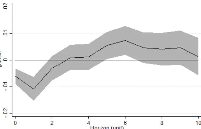
IRF suggests that the shock in the crisis dummy has an immediate negative effect on GDP
growth. In the year one after the crisis has ended the negative impact persists and reduces the
normal growth trend by around 1%. Two years after the crisis the effect has vanished and is
now insignificant, indicating that the economy of the country has recovered and is back on its
normal growth path. The IRF can not confirm the above average performance after two years
found when using the lagged crisis variable. After six years there is a slight positive significant
effect, but it is questionable if this is a consequence of the crisis event as many other factors
could be responsible for the effect. The result of an average recovery time of two years is robust
rather long time of 12 months pass until the economic engine of a country is at normal speed
again. A country suffers substantially under a systemic crisis as the recovery time together with
the average duration of a crisis sum up to more than half a decade of negative impact on GDP
growth.
9. Conclusion and Future Research Suggestions
The memorable images of long queues in front of British banks or Greek workers burning
down cars in outrage are not an exception. Analysing systemic crises among European countries
during almost 50 years reveals that financial crises have severe consequences for the average
citizen in the involved economies. A systemic crisis is connected to a growth decline of 1.8%
for each year that a country is caught up in the crisis. The impact proved to be robust even when
tested against a large set of control variables or different time frames. Previous research has
reported similar findings and a negative relation between crises and economic output is
undisputed. However, the reported size of the effect varies widely among different studies. The
here presented result is positioned on the lower end of the range of estimates. For comparison
Furceri and Zdzienicka (2011) reported that a debt crisis reduces output by around 6% per year.
The authors analysed a similar time span but included many more countries with a total of 154
observed economies. A large share of them are low developed countries or in the phase of Figure 1. The Response of GDP Growth to a Crisis
Note: IRF from Local Projection Method, response of GDP growth to shock in systemic crisis dummy. Black line represents the estimate, grey-shaded area is 95% confidence interval using robust standard errors.
emerging towards an advanced economy. Emerging markets being more vulnerable to external
shocks is thus a reasonable explanation for the large difference. Furthermore, the study worked
with the crisis definition of Laeven and Valencia who use a stricter definition for a crisis as
shown in section 3. This might influence the results as well but to a rather small extend as the
databases only differ slightly. A future research recommendation is to extend the presented
analysis in this paper to a broader set of countries including developing states as at the moment
only advanced countries are represented in the dataset used. This step would involve expanding
the ECB database to more countries.
Every crisis on its own has its special dynamics but there are repeating patterns which can
be categorized. The four main sources for crises were explained in section 4 and formed part of
a more detailed analysis of the impact on GDP of different crisis types. The Twin crises
Currency-Sovereign Debt, Currency-Asset Price Correction and Banking-Asset Price
Correction all showed to have a large significant negative impact on GDP growth. The panel
analysis showed that the interplay of both crises harms a country more than the case of just
suffering under the two components separately, which is a pure theoretical consideration.
Multiple crises where three or more risk factors materialised also prove to be especially harmful
for a country as the disruptions in one sector probably intensify the troubles in other areas. A
suggestion for further research is to closely analyse the channels through which the different
risk factors interact with each other and how such amplifying dynamics are created, in order to
find ways to mitigate the negative impacts of complex crises.
After a crisis has ended usually the confidence in the financial sector or the trustworthiness
of a government is shaken up. The involved actors often need to restructure as sometimes whole
departments of their business collapsed during the crisis. All this causes a certain recovery time until the country’s economy is back on track and can pick up the pre-crisis trend growth. Both
the analysis of a lagged crisis variable as well as the response function of growth to a shock in
To conclude, this thesis presented evidence to confirm the hypothesis that systemic crises
are harmful for economic output and delivered an estimate for the negative effect. Additionally,
a highly significant marginal negative impact of Twin crises and complex crises is reported.
The existence of a post-crisis recovery time could be confirmed with an estimated length of two
years.
Bibliography
Arellano, Manuel and Stephen Bond. 1991. “Some tests of specification for panel data: Monte Carlo evidence and an application to employment equations” Review of Economic Studies 58 (2): 277
Baynes, Chris. 2018. “Greece bailout programme finally comes to an end - but country faces decades of austerity.” The Independent. Accessed 8 November 2019.
https://www.independent.co.uk/news/world/europe/greece-eurozone-bailout-programme-end-alexis-tsipras-euro-europe-debt-austerity-a8498501.html
Bordo, Michael, Barry Eichengreen, Daniela Klingebiel, and Maria Soledad Martinez-Peria. 2001. “Is the Crisis Problem Growing More Severe?” Economic Policy 16 (April): 51– 82.
Caner, Mehmet, Thomas Grennes, and Fritzi Koehler-Geib. 2010. “Finding the Tipping Point - When Sovereign Debt Turns Bad.” World Bank Policy Research Working Paper No. 5391
Caprio, Gerard, Jr., and Daniela Klingebiel. 1996. “Bank Insolvencies: Cross-Country Experience.” World Bank Policy Research Working Paper No. 1620
Demirgüç-Kunt, Asli, and Enrica Detragiache. 1998. “The Determinants of Banking Crises in Developing and Developed Countries.” IMF Staff Papers Vol. 45, No. 1 March
Dell’Ariccia, Giovanni, Enrica Detragiache, and Raghuram Rajan. 2005. “The Real Effect of Banking Crises.” IMF Working Paper No. 05/63
Driscoll, John, and Aart Kraay. 1998. “Consistent Covariance Matrix Estimation With Spatially Dependent Panel Data.” The Review of Economics and Statistics Vol. 80, issue 4, 549-560
ECB. 2017. “A new database for financial crises in European countries.” Occasional Paper Series, No 13 / July
Eurostat. 2009. “Impact of the economic crisis on unemployment.” Statistics explained. Accessed 12 November 2019. https://ec.europa.eu/eurostat/statistics- explained /index.php/Archive:Impact_of_the_economic_crisis_on_unemployment
Furceri, Davide and Aleksandra Zdzienicka. 2011. “How Costly Are Debt Crises?” IMF Working Paper WP/11/280
Fratianni, Michele and Michael J. Artis. 1996. “The lira and the pound in the 1992 currency crisis: Fundamentals or speculation?“ Open Economies Review. March 1996. Volume 7, Supplement 1, pp 573-589
Hutchison, Michael M., and Ilan Noy. 2005. “How Bad Are Twins? Output Costs of Currency and Banking Crises.” Journal of Money Credit and Banking Vol. 37(4), pp. 725-52.
Jordà, Òscar. 2005. “Estimation and Inference of Impulse Responses by Local Projections.” American Economic Review Vol. 95 No. 1 161–82
Jordà, Òscar, Moritz Schularick, and Alan M. Taylor. 2013. “When Credit Bites Back.” Journal of Money, Credit and Banking 45 (December, Supplement): 3–28.
Krugman, Paul. 2007. “Will There Be a Dollar Crisis?” Economic Policy Vol. 22 No. 51
Laeven, Luc, and Fabián Valencia. 2008. “Systemic Banking Crises: A New Database.” IMF Working Paper WP/08/224
Laeven, Luc, and Fabián Valencia. 2013. “Systemic Banking Crises Database.” IMF Economic Review 61 (June): 225–270.
Oulton, Nicholas, and Maria Sebastiá-Barriel. 2017. “Effects of financial crises on
productivity, capital and employment.” LSE Research Online Documents on Economics 68541, London School of Economics and Political Science
Reinhart, Carmen M., and Kenneth S. Rogoff. 2009. This Time Is Different: Eight Centuries of Financial Folly. Princeton, NJ: Princeton University Press.
Reinhart, Carmen M., and Kenneth S. Rogoff. 2014. “Recovery from Financial Crises: Evidence from 100 Episodes.” NBER Working Paper No. 19823
Romer, Christina D., and David H. Romer. 2015. “New Evidence on the Impact of Financial Crises in Advanced Countries.” NBER Working Paper No. 21021 March
Teulings, Coen N. and Nikolay Zubanov. 2014. “Is Economic Recovery a Myth? Robust Estimation of Impulse Responses.” Journal of Applied Econometrics 29; 497-514
The New York Times. 2016. “Explaining Greece’s Debt Crisis.” Accessed 8 November 2019. https://www.nytimes.com/interactive/2016/business/international/greece-debt-crisis-euro.html
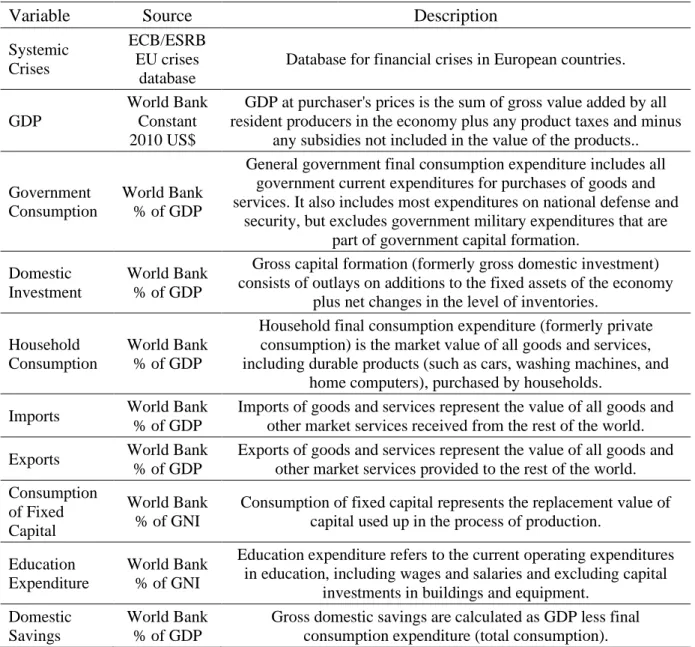
Appendix B
Table 3. Data Description
Variable Source Description
Systemic Crises
ECB/ESRB EU crises
database
Database for financial crises in European countries.
GDP
World Bank Constant 2010 US$
GDP at purchaser's prices is the sum of gross value added by all resident producers in the economy plus any product taxes and minus
any subsidies not included in the value of the products.. Government
Consumption
World Bank % of GDP
General government final consumption expenditure includes all government current expenditures for purchases of goods and services. It also includes most expenditures on national defense and
security, but excludes government military expenditures that are part of government capital formation.
Domestic Investment
World Bank % of GDP
Gross capital formation (formerly gross domestic investment) consists of outlays on additions to the fixed assets of the economy
plus net changes in the level of inventories. Household
Consumption
World Bank % of GDP
Household final consumption expenditure (formerly private consumption) is the market value of all goods and services, including durable products (such as cars, washing machines, and
home computers), purchased by households. Imports World Bank
% of GDP
Imports of goods and services represent the value of all goods and other market services received from the rest of the world. Exports World Bank
% of GDP
Exports of goods and services represent the value of all goods and other market services provided to the rest of the world. Consumption
of Fixed Capital
World Bank % of GNI
Consumption of fixed capital represents the replacement value of capital used up in the process of production.
Education Expenditure
World Bank % of GNI
Education expenditure refers to the current operating expenditures in education, including wages and salaries and excluding capital
investments in buildings and equipment. Domestic
Savings
World Bank % of GDP
Gross domestic savings are calculated as GDP less final consumption expenditure (total consumption).
Table 4. Diagnostic Tests
Diagnositc Tests mentioned in section 4 Methodology
Test Test Statistic p-value
F test that all 𝑢𝑖 = 0 F(15,727) = 4.35 0.0000
Breusch and Pagan Lagrangian multiplier test
for random effects 𝜒̅1
2 = 17.23 0.0000
Hausman Test 𝜒92 = 33.26 0.0001
Modified Wald test for groupwise
heteroskedasticity 𝜒16
2 = 187.86 0.0000
Wooldridge test for autocorrelation in panel
data F(1,15) = 71.322 0.0000
Breusch-Pagan LM test of cross sectional
independence 𝜒120
2 = 926.786 0.0000
Im-Pesaran-Shin unit-root test for GDP 𝑡̅ = -11.4056 0.0000 Im-Pesaran-Shin unit-root test for Systemic
Crisis 𝑡̅ = -4.9751 0.0000
Im-Pesaran-Shin unit-root test for Government
Consumption (Time trend included) 𝑡̅ = -1.4085 0.0795 Im-Pesaran-Shin unit-root test for Domestic
Investment 𝑡̅ = -3.6772 0.0001
Im-Pesaran-Shin unit-root test for Household
Consumption 𝑡̅ = -1.6307 0.0515
Table 5. Additional Regressions
(I) (II) Residual Event -0.0126 (-5.67)*** Systemic Crisis -0.0225 (-3.78)*** Government Consumption -0.0050 (-5.76)*** -0.0028 (-1.48)* Domestic Investment 0.0012 (2.57)** 0.0021 (4.90)*** Household Consumption -0.0005 (-1.18) 0.000 (0.04) N 752 319 within R2 0.29 0.25
Note: Driscoll-Kraay standard errors in brackets; * p < 0.1, ** p < 0.05, *** p < 0.01. (I): 1970 – 2017, 16 Countries. (II): 1995 – 2006, 29 Countries. All regressions include country fixed effects.