For
Jury
Ev
aluation
F
ACULDADE DEE
NGENHARIA DAU
NIVERSIDADE DOP
ORTOChurn Prediction in the Telecom
Business
Georgina Cunha Esteves
Mestrado Integrado em Engenharia Informática e Computação Supervisor: João Pedro Mendes Moreira
Churn Prediction in the Telecom Business
Georgina Cunha Esteves
Mestrado Integrado em Engenharia Informática e Computação
Approved in oral examination by the committee:
Chair: Doctor Name of the President
External Examiner: Doctor Name of the Examiner Supervisor: João Pedro Mendes Moreira
Abstract
Telecommunication companies are acknowledging the existing connection between customer sat-isfaction and company revenues. Customer churn in telecom refers to a customer that ceases his relationship with a company. Besides losing the customer, it is also likely that the customer will join a competitor company. These companies rely on three main strategies to generate more revenue: acquire new customers, upsell the existing ones or increase customer retention. Some articles suggest that churn prediction in telecom has recently gained substantial interest of stake-holders, who noticed that retaining a customer is substantially cheaper that gaining a new one. This dissertation compares six approaches that identify the clients who are closer to abandon their telecom provider. Those algorithms are: KNN, Naive Bayes, J48, Random Forest, AdaBoost and ANN. For the purpose of this research, real data was provided by WeDo technologies, which is the number one provider of revenue assurance and fraud management software for telecom oper-ators. The use of real data extended the refinement time necessary, but ensured that the developed algorithm and model can be applied to real world situations. The large dataset available opens a new set of possibilities, and makes it possible to obtain interesting and novel results. The models were evaluated according to three criteria: area under curve, sensitivity and specificity, with spe-cial weight to the first two values. The Random Forest algorithm proved to be the most adequate in all the test cases.
Keywords: Churn Prediction; Telecom; Machine Learning; Churn Analysis; Customer attri-tions analysis; Customer attriattri-tions.
Resumo
As empresas na área das telecomunicações estão a aperceber-se da forte ligação existente entre a satisfação do cliente e as receitas da empresa. Churn de clientes na área das telecomunicações refere-se a um cliente que cessa o contrato mantido com uma empresa. Além de perder o cliente, é também provável que o cliente irá juntar-se de uma empresa concorrente. As empresas contam com três estratégias principais para gerar mais receita: adquirir novos clientes, vender um novo serviço a clientes da empresa ou aumentar a retenção de clientes. Alguns artigos sugerem que a previsão de churn na áre das telecomunicações ganhou recentemente interesse substancial por parte das empresas, que notaram que reter um cliente é substancialmente mais barato do que adquirir um novo. Esta dissertação compara seis abordagens que identificam os clientes que estão mais perto de abandonar o seu fornecedor de telecomunicações. Esses algoritmos são: KNN, Naive Bayes, C4.5, Random Forest, AdaBoost e ANN. Para a realização desta pesquisa foram-nos fornecidos dados de clientes reais pela Wedo technologies, uma empresa que se especializou no fornecimento de software e consultoria especializada para analisar de forma inteligente grandes quantidades de dados de uma organização. O uso de dados reais prolongou a fase de refinamento de dados, mas garantiu que os algoritmos e modelos desenvolvidos podem ser aplicado a situações reais. O grande conjunto de dados disponível abre um novo conjunto de possibilidades, e faz com que seja possível obter resultados interessantes e inovadores. Os modelos foram avaliados de acordo com três critérios: áres sob curva, sensibilidade e especificidade, com peso especial para os primeiros dois valores. O algoritmo random forest provou ser o mais adequado em todos os casos de teste.
Keywords: Previsão de churn; Telecomunicações; Machine Learning; Análise de churn; Churn clientes.
Acknowledgements
I would like to thank my supervisor, Professor João Moreira, for his work and invaluable advice. I would also like to thank all of my friends who have motivated me and taught me over the past years. I thank Rui for his support during the last years. Without him by my side, i would not have reached this far. A special thanks to my parents and family. Your effort made me accomplish this goal.
“It’s kind of fun to do the impossible.”
Contents
1 Introduction 1
1.1 Context . . . 2
1.2 Motivation and Goals . . . 2
1.3 Dissertation Structure . . . 3
2 Literature Review on Churn Prediction 5 2.1 Customer Churn . . . 5
2.2 Data Mining . . . 6
2.3 Predictive modeling . . . 7
2.3.1 Regression . . . 7
2.3.2 Classification . . . 8
2.4 Churn Prediction Approaches . . . 13
2.4.1 Decision tree . . . 13
2.4.2 Logistic Regression . . . 14
2.4.3 Neural Network . . . 14
2.4.4 Support vector machines . . . 15
2.4.5 Multiple methods . . . 15
2.5 Data Preprocessing . . . 15
2.5.1 Data Problems . . . 15
2.5.2 Data Preprocessing techniques . . . 16
2.6 Conclusion . . . 17 3 Dataset 19 3.1 Data collection . . . 19 3.2 Data selection . . . 19 3.3 Data analysis . . . 20 3.4 Data transformation . . . 27
4 Implementation and Results 29 4.1 Experimental Setup . . . 29 4.2 Results . . . 32 4.2.1 Knn . . . 32 4.2.2 Naive Bayes . . . 35 4.2.3 Random Forest . . . 37 4.2.4 C4.5 . . . 40 4.2.5 AdaBoost . . . 42 4.2.6 ANN . . . 45 4.3 Model Comparison . . . 48
CONTENTS
4.3.1 Variable importance . . . 54
5 Conclusions and Future Work 55
5.1 Conclusions . . . 55
5.2 Future Work . . . 56
References 59
A Results 63
List of Figures
2.1 Data mining process . . . 6
2.2 Neural Network . . . 13
3.1 Data structure . . . 20
3.2 Data summary . . . 21
3.3 Number of calls per call duration . . . 21
3.4 Call direction . . . 22
3.5 Call type . . . 23
3.6 Call destination . . . 24
3.7 Dropped calls . . . 24
3.8 Days without calls . . . 25
3.9 Churn distribution . . . 26
3.10 Data structure after type conversion . . . 27
3.11 Summary of new data . . . 27
4.1 Knn ROC value per number of neighbors . . . 33
4.2 Knn model ROC curve . . . 34
4.3 Naive Bayes ROC curve . . . 36
4.4 Random Forest number of predictors . . . 37
4.5 Random Forest ROC curve . . . 39
4.6 J48 ROC curve . . . 41
4.7 AdaBoost parameter study . . . 43
4.8 AdaBoost ROC curve . . . 44
4.9 ANN parameter study . . . 46
4.10 ANN ROC curve . . . 47
4.11 ROC values box plot . . . 49
4.12 Sensitivity values box plot . . . 51
4.13 ROC values differences box plot . . . 52
4.14 Sensitivity values differences box plot . . . 53
A.1 Specificity values box plot . . . 63
A.2 ROC values dot plot . . . 64
A.3 Specificity comparison values box plot . . . 64
A.4 Model comparison dot plot . . . 65
List of Tables
2.1 Confusion matrix . . . 9
3.1 Variables in the data . . . 20
4.1 Dataset Sampling results . . . 30
4.2 Models P-values . . . 48
4.3 AUC value comparison . . . 49
4.4 Sensitivity value comparison . . . 50
Abbreviations
ANN Artificial Neural Network AUC Area Under Curve
ARD Automatic Relevance Determination
FEUP Faculdade de Engenharia da Universidade do Porto FN False Negatives
FP False Positives
HPC High Performance Computing IDE Integrated Development Environment KNN K-nearest neighbors
MAE Mean Absolute Error
PCC Percentage of correctly classified RMSE Root Mean Square Error
ROC Receiver operating characteristic
SMOTE Synthetic Minority Over-sampling Technique SVM Support Vector Machine
TP True Positives TN True Negatives
Chapter 1
Introduction
2Since the 1990s the telecommunications sector became one of the key areas to the development
4
of industrialized nations. The main boosters were technical progress, the increasing number of operators and the arrival of competition. This importance has been accompanied by an increase in
6
published studies sector and more specifically on marketing strategies [Gerpott et al., 2001]. In order to acquire new costumers, a company must invest significant resources to provide
8
a product or service that stands out from the competitors, however, continuously evolving the product itself is not enough. Many companies are embracing new strategies based on data mining
10
techniques to survive in this ever-increasing competitive market. These techniques are addressing challenging problems such as prospect profiling, fraud detection, and churn prediction. Churn
12
refers to “the costumer movement from one provider to another” [Bott, 2014]. The ability to predict this variable is a concern of a broad number of industries, but it is mainly being focused
14
by telecommunication service providers. There are several factors that justify this interest by telecom companies: the vast offer of similar products by multiple companies, along with the ease
16
in changing operators and the Mobile Number Portability allow costumers to switch to another telecom provider effortless and still maintain their telephone number.
18
Companies were very fond of discovering the correlation between this new development and their profit, so they conducted a few studies [Wei and Chiu, 2002, Ascarza et al., 2016]. Three
20
main strategies to generate more revenue were identified [Wei and Chiu, 2002]: acquire new cus-tomers, upsell the existing ones or increase customer retention. All these strategies will be
com-22
pared using the return on investment value (ratio between extra revenue that results from these efforts and their cost). Gaining new customers is a well-known strategy in all markets to increase
24
income. If a company is able to sell a product or service to a new customer, the profits of the com-pany increase. However, this is considered to be an extremely expensive approach. The investment
26
made regarding money, time and effort (new account setup, credit searches, and advertising and promotional expenses) is not so appealing when compared with the revenue produced. The second
28
Introduction
is already associated with the company, and he simply expands his current service or product to a more expensive one. But as seen in recent studies [Zaki and Meira, 2013], it is not an easy task 2
to convince a customer to upgrade their current service. A big gain to the client must be present for them to consider this change. The strategy that was described as the most profitable (great- 4
est return on investment) was increasing customer retention [Wei and Chiu, 2002]. The company profits in two ways when retaining a customer: they continue to generate revenue to the company 6
by purchasing their service, and the competitors company does not gain strength in the market by
gaining a new customer. 8
There are a vast number of strategies to improve customer retention overall. By simply talking to customers and conduct customer satisfaction surveys, a lot of problems regarding the customer- 10
company relationship can be identified. But when the company wants to individualize customer retention, a new problem appears: a company has a great number of clients, and can not afford 12
to spend a lot of time with each one of them. This is where Data Mining becomes useful: by predicting in advance when and which customers are at risk of leaving the company, all the efforts 14
to retain customers could be addressed to these cases.
1.1
Context
16Telecom companies are starting to realise the effectiveness of churn prediction as a way of gen-erating more profit, specially when compared to other approaches. An increasing investment was 18
made in the study area of churn prediction during past years [Ascarza et al., 2016]. In the context of a collaboration between FEUP and WeDo Technologies, an exploration of methods to detect 20
which clients are close to change their telecom operator (churning) was conducted. WeDo tech-nologies is the number one provider of revenue assurance and fraud management software for 22
telecom operators [WeDoTechnologies,]. This area is of great interest for this kind of companies, because the costs of maintaining a current customer are typically lower than the costs of acquiring 24
a new client[Reinartz and Kumar, 2002]. Churn prediction must be interpreted as a different prob-lem for each company, because each business area has different indicators that must be identified 26
to detect how attached a client is to the current operator.
1.2
Motivation and Goals
28The objective of this dissertation is to develop a method for churn prediction in the telecom busi-ness. The intended result is an algorithm that identifies the clients that are closer to abandon their 30
current operator. Although many approaches were conducted in the past few years, there are still many opportunities to improve the current work in this area. The data that will be used during this 32
work is fundamental to assure the quality of the final solution. The dataset is an extend collection of calls conducted by real customers. This will extend the refinement time necessary, but will 34
ensure that the developed algorithm and model can be applied to real world situations. It opens a new set of possibilities, and makes it possible to obtain interesting and novel results. 36
Introduction
There are several desired requirements in a churn prediction system. According to the author [Balle et al., 2013], those requirements are the following:
2
• Precision and Recall - high level of recall (almost all churners must be identified) and medium-high level of precision (low number of false positives).
4
• Performance - the execution speed of the model with new data. This is essential for the company to be able to tale the right decisions at the right time.
6
• Flexibility - the model must be able to keep up with good forecast rates with new data. It should take into account changes in customers patterns when making the predictions.
8
• Scalability - the model needs to react positively if the data intake increases.
• Targeting: this feature relates to the ability to identify concrete data on the users more likely
10
to leave the service.
All the requirements previously mentioned are taken into account when developing the
solu-12
tion to this problem. The most intricate requirement to achieve are the ones regarding the execution speed and model performance. Due to the big amount of available data to develop our solution,
14
some of the tested algorithms take a considerable amount of time to complete. To neutralize this negative situation, we adopted a strategy based on parallel computation. In this way, the
process-16
ing is distributed among the available cores, splitting the processing time by the number of cores (in the optimal scenario).
18
1.3
Dissertation Structure
Besides this introductory chapter, this dissertation contains 3 more chapters. In chapter 2, a
20
review of the existing literature on the topic is conducted and some related work is presented. Several algorithms are detailed and explained, and data preprocessing importance and techniques
22
are compared.
In chapter 3, an initial view around implementation details is made. An overview of the
24
dataset and its variables is conducted, as well as the main operations made upon the data. Chapter 4contains the experimental setup definition and final results acquired.
26
Lastly, chapter 5contains the main conclusions of this research, some ideas regarding future work.
Chapter 2
Literature Review on Churn Prediction
2In this chapter a review of the bibliographic content found is conducted. The main focus are the
4
approaches and techniques applied to churn prediction in telecom businesses, as well as some data preprocessing techniques and problems.
6
2.1
Customer Churn
According to the author [Yen and Wang, 2006], ’costumer churn’ in telecom business refers to
8
the costumer movement from one provider to another. ’Customer management’ is the process conducted by a telecom company to retain profitable costumers.
10
The continuous evolution of technology has opened up the telecommunications industry, mak-ing this market more competitive than ever. These companies are realizmak-ing that a
customer-12
oriented business strategy is crucial for sustaining their profit and preserving their competitive edge [Tsai and Lu, 2009]. As acquiring a new costumer can add up to several times the cost
14
of efforts that might enable the firms to retain a customer, a best core marketing strategy has been followed by most in the telecom market: retain existing customers, avoiding customer churn
16
[Kim and Yoon, 2004,Kim et al., 2004].
Two main types of targeted approaches to manage customer churn [Tsai and Lu, 2009] were
18
identified: reactive and proactive. In the reactive approach, the company waits until the customer asks to cease their contract to act. In this situation, the company will then offer some advantages
20
and incentives to retain the customer. The other approach is the proactive approach, where a company tries to identify which customers are more likely to churn before they do so. In this case,
22
the company provides special offers to keep them from churning.
A few studies have been conducted to evaluate which is the approach, reactive or proactive, is
24
better to a company. A majority of them agreed that the proactive approach achieves better results [Retana et al., 2016,Olaleke et al., 2014], and the work developed in this project will be based in
Literature Review on Churn Prediction
this second approach. The main objective is to predict beforehand the customers more likely to
churn using data mining techniques. 2
In the scope of this project, a distinction between types of churn must be made. Involuntary churn is when circumstances outside the user and service provider’s control affect the decision of 4
ceasing their relationship. Customers’ relocation to a distant location and death are part of this kind of churn. Voluntary churn is when a customer actively decides to leave the product or service 6
of a company. Involuntary churn tends to be discarded to churn prediction, because those are the ones that do not represent the company-customer relationship. 8
2.2
Data Mining
The author [Yen and Wang, 2006] stated that data mining can be defined as ‘the extraction of 10
hidden predictive information from large databases’. It can be defined as a logical process that is used to search through large amount of data with the objective of finding useful information. 12
The main goal of this technique is to find patterns that were previously unknown as well as novel information. This new information can be used by company owners to make adequate decisions 14
to the companies future.
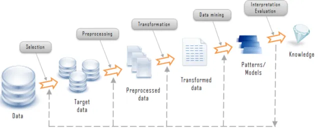
Figure 2.1: Data mining process
In Figure2.1a typical data mining process is described. That process can be simplified into 16
three major steps: exploration, pattern identification and deployment. The first step is mainly focused on the data. It must be explored, cleaned and transformed (if necessary) to other forms of 18
representation. Non-interesting data can also be discarded during this phase.
Once the data is explored and refined, a pattern identification must be formed. These patterns 20
must be identified and chosen based on their performance on the prediction.
The last step regards the deployment of the patterns previously mentioned. The outcome must 22
Literature Review on Churn Prediction
Data mining is, in fact, a new technology that has the potential to help the process of explo-ration of vast quantities of data.
2
When dealing with data from a big telecom company, only depending on human preprocessing effort is not efficient. With millions of clients and an ever bigger magnitude in the number of
4
telephone calls, the process of scanning through all this information with only human intervention is both expensive and inefficient [Ngai et al., 2009]. The emerging data mining tools can answer
6
this kind of problems. If the dataset has a sufficient size and quality, data mining technology can provide business intelligence to generate new opportunities [Yen and Wang, 2006].
8
2.3
Predictive modeling
In data mining, predictive modeling is the process of creating a model to predict an outcome. To
10
do so, the past must be analyzed and, with this information, the model must be constructed and validated. In order to create this model there must be predictors, which are variable factors that
12
expected to influence future behavior. For example, when predicting churn these factors can be number of calls to the operator assistance or the number of dropped calls regarding a certain client.
14
If the outcome is qualitative it is called classification and if the outcome is quantitative it is named regression. Descriptive modeling or clustering is the assignment of observations into clusters
16
so that observations in the same cluster are similar. Finally, association rules can find interesting associations amongst observations. The following sections will describe these techniques in detail,
18
and identify specific types for each one.
2.3.1 Regression 20
Regression is a data mining function that predicts a numeric value. It can be used to model the rela-tionship between one or more independent variables and dependent variables[Zaki and Meira, 2013].
22
For example: it could be used to predict children’s height given their age and weight. In order to apply regression to a dataset, the target values must be known. Using the same example as
24
above: to predict children’s height, there must exist data during a period of time regarding their age, height, weight, and others. Height is then considered the target variable, and all the other
26
attributes would be predictors.
During the model training process, a regression algorithm determines the value of the target.
28
This value is assessed as a function of the predictors. The multiple iterations of this step threw all of the initial data compose a model. Later, this model can be applied to a different dataset with the
30
unknown target values.
To better understand how regression works, a few basic concepts will be detailed. As already
32
mentioned, the goal of regression analysis is to find the values of parameters in which the function best fits a set of provided data. The following equation represents this approach. The value of the
34
continuous target variable (y) is the value of a function F according to predictors(x) and a set of patameters p. An error measure e is also taken into consideration, to minimize the possibility of
36
Literature Review on Churn Prediction
y= F(x, p) + e (2.1)
Four main groups of Regression algorithms are:
1. Frequency Table 2
• Decision Tree
2. Covariance Matrix 4
• Multiple Linear Regression
3. Similarity Functions 6
• K Nearest Neighbors
4. Others 8
• Artificial Neural Network
• Support Vector Machine 10
The testing of regression models involves calculating multiple statistics. These statistics rep-resent the difference between the predicted and the expected values. 12
Two of the most applied measures when testing a regression model [Shao and Deng, 2016] are Mean Absolute Error (MAE) and Root Mean Squared Error (RMSE). 14
The MAE is an average of the absolute errors. This value is given by
MAE=1 n n
∑
i=1 | fi− yi| (2.2)where fi is the predicted value and yi is the true value. 16
RMSE is the square root of the mean of the square of all of the error. The formula for RMSE
is 18 RMSE= s 1 n n
∑
i=1 (yi− ˆyi)2 (2.3)The use of RMSE is very common and it makes an excellent general purpose error metric for
numerical predictions. 20
Compared to the previously detailed MAE, RMSE amplifies and punishes large errors.
2.3.2 Classification 22
Classification is a data mining task of predicting the value of a categorical variable (target or class) by building a model based on one or more numerical and/or categorical variables (predictors or 24
Literature Review on Churn Prediction
a set of inputs. In order to predict this, the algorithm processes a training set containing several attributes and their respective outcome (prediction attribute). It then tries to discover relationships
2
between these attributes that lead to predicting the outcome. Next, a new set must be taken into consideration: the prediction set. This is composed of new data (unknown to the algorithm) with
4
the same attributes as the training set except for the prediction attribute. The algorithm produces a prediction based on this new data, and an accuracy value defines how "good" the algorithm is.
6
Applications regarding fraud detection and credit-risk are normally connected to this technique. Classification algorithms can be stratified into four main groups:
8 1. Frequency Table • ZeroR 10 • OneR • Naive Bayesian 12 • Decision Tree 2. Covariance Matrix 14
• Linear Discriminant Analysis • Logistic Regression 16 3. Similarity Functions • K Nearest Neighbors 18 4. Others
• Artificial Neural Network
20
• Support Vector Machine
Table 2.1: Confusion matrix Predicted Non churn Churn
Actual Positive TP FN
Negative FP TN
In order to assess the developed models, evaluation methods must be applied. The confusion
22
matrix showed in table2.1contains information about actual and predicted classifications done by a classification system.
24
Each term corresponds to a specific case:
• True positives (TP): These are cases in which the prediction is yes (the client did not left
26
Literature Review on Churn Prediction
• True negatives (TN): The prediction is no, and they churned (left the company).
• False positives (FP): The prediction is yes, but the client left the company. (Also known as 2
a "Type I error.")
• False negatives (FN): The prediction is no, but the client actually stayed in the company. 4
(Also known as a "Type II error.")
The two types of errors the model can commit, FP and FN, will also have different weights in 6
the system. It is worse to a telecom company not to predict a customer that is going to churn, than
to address one that does not plan to leave the company. 8
Three criteria will be used to evaluate the system: accuracy, hit rate and churn rate.
Accuracy measures the rate of the correctly classified instances of both classes. The formula 10
is:
Accuracy= T P+ T N
T P+ FN + FP + T N (2.4)
Hit rate gives us an index of the rate of predicted churn in actual churn and actual non-churn. 12
It is represented by:
HitRate= T N
FN+ T N (2.5)
Churn rate measures the rate of predicted churn in actual churn. The formula is: 14
ChurnRate= T N
FP+ T N (2.6)
2.3.2.1 K Nearest Neighbors
K Nearest Neighbors (KNN) is a simple algorithm that collects all available cases and classifies 16
new cases based on a similarity measure. KNN has been used in statistical estimation and pattern recognition since the beginning of 1970’s as a non-parametric technique. 18
The process of assigning a class to a new case follow these steps:
1. Find k nearest neighbors of the new case in the existing dataset, according to some distance 20
or similarity measure. It compares the new sample to all known samples in the existing dataset and determines which k known samples are most similar to it. K value is determined 22
beforehand.
2. Determine which class value is the one most of those k known samples belong. 24
3. Assign the determined class to the new sample.
If the target variable is categorical, there are three most used distance measures: Euclidean, 26
Manhattan and Minkowski.
In the instance of categorical variables the Hamming distance must be used. This measure is 28
calculated according to the following equation.
DH= k
∑
i=1
Literature Review on Churn Prediction
2.3.2.2 Naive Bayes
The Naive Bayesian classifier is based on Bayes’ theorem. It is a model easy to build, with no
2
complicated iterative parameter estimation, which makes it useful and practical for very large datasets. Despite its simplicity, the Naive Bayes classifier often does surprisingly well and is
4
widely used because it often outperforms more sophisticated classification methods.
Bayes theorem provides a way of calculating the posterior probability P(c|x). It assumes that
6
the effect of the value of a predictor (x) on a given class (c) is independent of the values of the other predictors. This assumption is called class conditional independence.
8
The posterior probability is calculated according to the following equation: P(c|x) = P(x|c)P(c)
P(x) (2.8)
Where:
10
• P(c | x) is the posterior probability of the target given predictor • P(x | c) is the probability of predictor given the target
12
• P(c) is the probability of target • P(x) is the probability of predictor
14
2.3.2.3 C4.5
C4.5 is an algorithm used to generate decision trees from a set of training data. Each node in the
16
tree corresponds to a non-categorical attribute and each arc to a possible value of that attribute. A leaf of the tree specifies the expected value of the categorical attribute for the records described by
18
the path from the root to that leaf.
At each node of the tree, the algorithm chooses the attribute of the data that most effectively
20
splits its set of samples into subsets. The splitting criterion is the normalized information gain. The attribute with the highest normalized information gain is chosen to make the decision upon.
22
Usually the category attribute takes only the values true, false, or something similar where one of its values represents failure.
24
Regarding the algorithms behavior, we can describe 3 base cases:
• All the samples belong to the same class; in this case, the algorithm creates a leaf node
26
saying to choose that class.
• None of the analyzed features provides information gain; in this case, C4.5 creates a node
28
higher up on the decision tree with the expected value of the class.
• Finds an instance of previously unseen class; the algorithm behaves the same way as in the
30
Literature Review on Churn Prediction
2.3.2.4 Random Forest
Random Forest is a technique that grows many classification trees. The growth of each tree follows 2
the steps:
1. Considering N the number of cases in the training set, sample N cases at random from the 4
original data to grow the trees.
2. Considering M as the number of input variables, a number m lower than M is specified. At 6
each node, m variables are selected and the best split on these m is used to split the node.
Value m is not altered during the trees growth. 8
3. Each tree is growth to largest extent possible without pruning the trees.
To classify a new individual, that individual is tested with all the previously generated trees. 10
Each tree gives a classification, and the classification that acquired the most number of votes is
considered to be correct for that individual. 12
2.3.2.5 AdaBoost
AdaBoost is a type of ensemble learning algorithm where multiple learners are employed to build 14
a stronger learning algorithm. It works by choosing a base algorithm (e.g. decision trees) and iteratively improving it by accounting for the incorrectly classified examples in the training set. 16
It operates in the following way:
1. Assign equal weights to all training examples and chose a base algorithm 18
2. At each step of iteration, apply the base algorithm to the training set and increase the weights
of the incorrectly classified examples 20
3. Iterate n times, each time applying base learner on the training set with updated weights
4. The final model is the weighted sum of the n learners 22
2.3.2.6 ANN
Artificial Neural networks can be interpreted as a brain metaphor for information processing. The 24
ability to learn from the data and to generalize have popularized this method. According to the author [Tsai and Lu, 2009], neural computing refers to a pattern recognition methodology for ma- 26
chine learning. The resulting model from neural computing is called artificial neural network (ANN). They are mostly applied in business applications for pattern recognition, forecasting, pre- 28
diction, and classification.
Figure2.2 represents the network structure of a ANN. It is composed of multiple neurons 30
grouped in three layers: input, hidden and output.
Literature Review on Churn Prediction
Figure 2.2: Neural Network
The hidden layer takes the inputs from the previous layer and converts them into outputs for further processing. This layer can be interpreted as a feature extraction mechanism.
2
The output layer contain the solution to a problem.
There can be multiple hidden layer in a ANN, but often just one is used.
4
The key element in a ANN are connection weights. They represent the relative importance of each input to a processing element. These weights are continuously adjusted, which allows the
6
learning process of the ANN.
2.4
Churn Prediction Approaches
8
The ability to predict that a particular customer has a high risk of churning, while there is still time to do something about it, represents a huge additional potential revenue source for every business.
10
So, a huge investment has been conducted in this area, and multiple approaches have been studied and tested.
12
The accuracy of the techniques used is critical to the success of any retention efforts. In the following sections, some of these technique applied to the churn problem will be presented.
14
2.4.1 Decision tree
Most customer segmentation methods are based on experience or Average Revenue per User, and
16
do not take into consideration customers’ future revenue or the cost of servicing customers of different types. A costumer evaluation by these methods may not be the most accurate. In this
18
approach [Han et al., 2012], a new way of customer segmentation is proposed. This model can be used to predict a customer lifecycle using only his demographic information. For each customer,
Literature Review on Churn Prediction
five decision models are applied: current value, historic value, prediction of long-term value, credit and loyalty. To compute loyalty and credit, an AHP (analytic hierarchy process) method is used. 2
For evaluating the accuracy of the model, the hit ratio of customer value is taken into
consid-eration. 4
2.4.2 Logistic Regression
This study [Oghojafor et al., 2012] uses logistic regression to examine the effect of socio-economic 6
factors on customer attrition. This is done by investigating the factors that influence subscribers churning one service provider for another. In this study, “Intention to drop current service provider” 8
is taken as the categorical response variable. The objective is to evaluate the impact of some de-mographic and socio-economic factors on the willingness to churn. These factors are age, sex, 10
marital status, education, income, occupational type, occupation and advertising medium.
Two models were constructed in this research. The first one used the most common factors 12
in churn prediction to construct the model, such as call expenses, type of service and number of mobile connection. The second model used the factors from the first model and a few more: the 14
demographic and socio-economic factors.
This approach concluded that most independent variables are highly significant to the predic- 16
tion, wich indicates a "strong relationship between the independent variables and the explanatory variable". High call rates and poor service facilities stand out among the identified churn determi- 18
nants.
2.4.3 Neural Network 20
Hybrid data mining techniques combining two or more techniques have been gaining visibility. In a vast number of problem domains, these techniques are proving to provide better performances 22
than single techniques.
One of the studied approaches [Tsai and Lu, 2009] considers two hybrid models. It combines 24
two different neural network techniques for churn prediction: back-propagation artificial neural networks (ANN) and self- organizing maps (SOM). The hybrid models are ANN combined with 26
ANN and SOM combined with ANN. The first technique of the two models performs data reduc-tion task by filtering out unrepresentative training data. Then, the outputs are used to create the 28
prediction model based on the second technique. In order to evaluate the performance of these models, three different kinds of testing sets were developed. The experimental results showed that 30
the two hybrid models outperform the single neural network baseline model in terms of prediction accuracy and Types I and II errors over the three kinds of testing sets. 32
Another study [Bott, 2014] investigates the application of Multilayer Perceptron (MLP) neu-ral networks with back-propagation learning to identify the most influencing factors in costumer 34
churn. Two methods were examined and compared; the typical change on error method and the ANN weights based method. In both methods, three attributes were identified as important to the 36
Literature Review on Churn Prediction
prediction by both models. These attributes are total monthly fees, total of international outgoing calls and 3G service.
2
2.4.4 Support vector machines
One of the studied approaches[Coussement and Poel, 2008] consisted on applying SVM to a
news-4
paper subscription churn context. The objective was to construct an accurate churn model using and tunning this technique. The customer churn prediction performance of the model was
bench-6
marked to logistic regression and random forecasts.
The authors chose as the main metric to evaluate their models Area under curve (AUC). The
8
best value regarding their SVM models was 85.14, and the random forest model used as benchmark conquered a final AUC value of 87.21.
10
2.4.5 Multiple methods
According to our research literature regarding customer churn, the majority of the related work
12
focuses on applying only one data mining method to extract knowledge.
Only a few authors [Verbeke et al., 2012] focused on comparing multiple strategies to
pre-14
dict customer churn. One of the investigated studies [Buckinx and den Poel, 2005] consists on comparing three classification techniques: Logistic regression, automatic relevance determination
16
(ARD) Neural Networks and Random Forests. The models were evaluated regarding their AUC and percentage of correctly classified (PCC) instances, in both training and testing sets.
18
The highest AUC value was obtained by the Random Forest model in both train and test sets, with values 0.8249 and 0.8319 respectively.
20
2.5
Data Preprocessing
Data preprocessing is an important step on any data mining project. Real world data is generally
22
incomplete, inconsistent and even with errors. In order to produce a good model to a problem, these issues must be addressed. It will be discussed several data preprocessing issues and
tech-24
niques.
2.5.1 Data Problems 26
This section classifies the major data quality problems to be solved by data cleaning and data transformation. As we will see, these problems are closely related and should thus be treated in
28
a uniform way. Cleaning a target dataset can be an even heavier task then collecting the data
[Rahm and Do, 2000]. Data can contain several kinds of problems:
30
• Noise : The occurrence of noise in data is typically due to recording errors and technology limitations. In can also be connected to the uncertainty and probabilistic nature of specific
32
Literature Review on Churn Prediction
• Missing data : Missing data can occur due to multiple situations. There could be conflicts in the recorded data, which lead to overwritten data. In some cases, that specific field of the 2
data could not be considered important at the time and hence not captured.
• Redundant data : This kind of error is mostly related with human errors. The data could have 4
been recorded under different names or in different places. It can also be representative of records containing irrelevant or information-poor attributes. 6
• Insufficient and stale data : Sometimes the data that we need comes from rare events and hence we may have insufficient data. Sometimes the data may not be up to date and hence 8
we may need to discard it and may end up with insufficient data.
2.5.2 Data Preprocessing techniques 10
In order to improve the quality of the previously gathered data, several preprocessing techniques can be applied [Zaki and Meira, 2013]. These techniques can be divided into four major cate- 12
gories: data cleaning, data transformation, data reduction and data integration.
2.5.2.1 Data cleaning 14
Data cleaning techniques aim to clean the data by filling in missing values, dealing with outliers, smoothing noisy data and fixing inconsistencies. When the data contains missing values, a few 16
methods can be implemented to fix this issue. The most common approaches to solve this problem are ignoring the tuple, or fill in the missing value using the mean attribute. 18
If the data contains noise, some data smoothing techniques can be applied, including clustering
and regression methods. 20
Inconsistent data may be corrected through a paper trace method. Knowledge engineering tools can also be used to detect violations of known data constraints. 22
2.5.2.2 Data transformation
Data transformation consist in reconstructing the data into a new form more appropriate to the data 24
mining task. Several kinds of data transformation can be employed:
• Normalization 26
• Smoothing
• Data Generalization 28
• Aggregation
Normalization is one of the most used techniques to transform data. In the simplest case, it 30
means adjusting values that are measured on different scales to a common scale. It many cases,
Literature Review on Churn Prediction
2.5.2.3 Data reduction
Mining on big amounts of data can be a longstanding task, sometimes even unfeasible. Data
2
reduction techniques aim to reduce the quantity of data to be analyzed without compromising the integrity of the original data. It consists on reducing the volume of the data or its dimensionality,
4
by removing attributes. There are a few strategies for data reductions: • Data cube aggregation
6 • Data compression • Data reduction 8 • Numerosity reduction • Discretization 10 2.5.2.4 Data integration
Most of data analysis projects involve combining data from multiple source into a single data store.
12
This task is called data integration. Several challenges are presented when integrating multiple data sources. For example, the same attribute can have different names among the different sources,
14
and it may not have an intuitive name.
The best approach in this kind of task is to use the metadata usually present in databases and
16
warehouses to help avoid error in the integration.
2.6
Conclusion
18
Several predictive modeling approaches were studied and their main characteristics detailed. Be-sides this overview, a more detailed explanation of some authors approaches to predict churn is
20
presented. Most of the authors focus on training and testing one single model, tunning its param-eters to best fit their main objective.
22
We considered that an approach consisting of testing multiple algorithms and compare their re-sults would bring interesting rere-sults to our research. With this mindset, we selected six algorithms
24
from multiple backgrounds. Those algorithms are: • KNN 26 • Naive Bayes • Random Forest 28 • C4.5 (J48 implementation) • AdaBoost 30
Literature Review on Churn Prediction
• ANN
The choice of these algorithms took into consideration their popularity and efficiency among 2
the data mining community, as well as some studies that compare data mining approaches [Wu et al., 2008,
Fern and Cernadas, 2014] in classification problems. 4
Chapter3will focus the dataset itself, its analysis and some of the preprocessing techniques
Chapter 3
Dataset
2The models that predict customer churn are based on knowledge regarding the company’s clients and their calls. That information is stored in a database table and is called dataset.
4
All the models were trained and tested with this data. But before that can happen, this collec-tion had to go through multiple transformacollec-tions and pre-processing techniques to make it suitable
6
to predict upon.
This chapter aims to describe all the steps regarding data. It begins explaining how the data
8
was retrieved and stored, how we conducted the selection process of the needed information, its analysis and the main transformations performed to make it suitable to predict upon.
10
3.1
Data collection
For the purpose of this research, real data from WeDo technologies client calls was provided by
12
the company. The data is stored in a SQL file, and has a size of more than 131 gigabytes. The file contains one table with over 1.2 billion entries from 5 million different clients.
14
SQLite library[SQLite,] was chosen due to its speed and efficiency, and since it is the tech-nology adopted by the High Performance Computing (HPC) [FEUP,] at Faculdade de Engenharia
16
Universidade do Porto (FEUP) . HPC is a research tool that can be used to solve complex com-putational problems. This technology added great value to our development process, because it
18
provided great computational power that enabled faster processing times.
3.2
Data selection
20
Due to computational and time limitations, the dataset available to this research was too large and needed to be sampled. In order to prevent the lost of valuable information and keep the final results
22
accurate, a simple selection of the first N table entries was not viable. The right approach to this problem is to retrieve all the call records from a group of clients. The query employed to divide
24
the database was the following:
Dataset
1 SELECT * FROM call_details AS c INNER JOIN
2 (SELECT DISTINCT(contract_id) FROM ( 2
3 SELECT * FROM call_details LIMIT 1000000))
4 AS v ON c.contract_id = v.contract_id; 4
In this way, we the dataset consists of entire history of a percentage of the total number of 6
clients to predict upon. The final dataset generated by this query contained over 100 thousand
calls between 30 June 2012 and 31 January 2013. 8
3.3
Data analysis
The dataset available to this research contains information regarding call information of telecom 10
company clients.
Table 3.1: Variables in the data
Variable Value Description DATE YearMonthDay Date of the call TIME HoursMinutesSeconds Time of the call DURATION Seconds Call duration
MSISDN Numeric Anonymized number. If Incoming, it is the number getting the call. If Outgoing, is the number calling. OTHER_MSISDN Numeric The "other" number in the call (regarding the previous variable).
CONTRACT_ID Numeric Client code
OTHER_CONTRACT_ID Numeric Not present in all data (does not belong to the operator). START_CELL_ID Numeric Should represent the calling device (Outgoing). END_CELL_ID Numeric Should represent the device getting the call (Ingoing). DIRECTION I, O Represent a incoming call,("I") or outgoing,("O"). CALL_TYPE FI, MO, ON, OT, SV
FI - The other device in the call bellongs to a wireline MO - The other device in the call bellongs to amobile network ON - On-Net, both incoming and outgoing systems bellong to this operator OT - Others
SV - Services:VoiceMail calls, etc DESTINATION_TYPE I, L Local (L) or international (I) desteny. DROPPED_CALL Y, N Dropped call (Yes or No) VOICMAIL Y, N Call went to voicemail (Yes or No)
Dataset
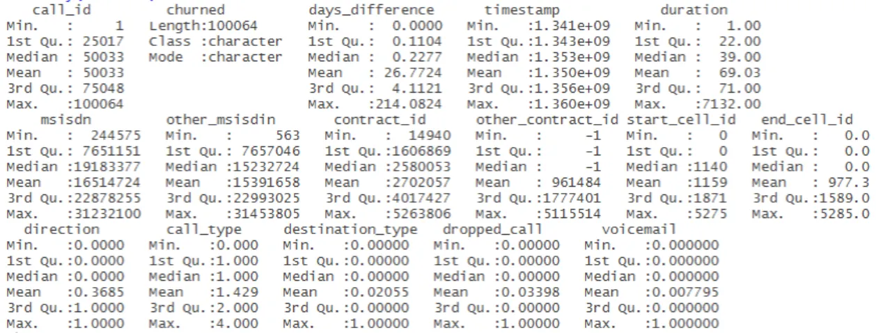
Table3.1contains an overview of the data. It identifies the variables, their values and a simple description of their meaning.
2
To explore data and also to implement and evaluate the algorithms we chose R language and environment [Foundation,]. This data was stored in a data frame, and contains categorical
(char-4
acter) and continuous (numeric) values. A variety of useful functions to explore the data frame were applied, namely str() and summary() functions.
6
The str() function returns a compact display of the internal structure of the data frame. It returns a few example outputs and the types of data for each column. As represented in3.1, there
8
are two types of variables: int, which are the integer variables; and chr, representing the character variables.
10
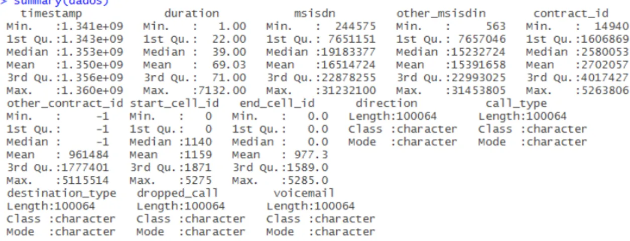
Figure 3.2: Data summary
Dataset
summary()is a generic function used to produce result summaries of data. When applied to a data frame, it is applied to each column, and the results for all columns are shown together. The 2
results of this function applied to the data are shown in3.2. As the values were not yet transformed into proper data types, some of the columns are not interpreted the right way, such as "timestamp". 4
In the variable "duration", the maximum value is extremely high when compared to that variables’
mean. 6
To acquire a better understanding of some of the data variables, we used Tableau Desktop[Software,] software. Tableau is a data visualization and communication tool widely used around the world. 8
It can import in an easy and quick way data from multiple file formats, including R objects.
Figure3.3is a visual representation of the duration in minutes of client calls. The calls were 10
group in 20 minutes intervals. The graph was also trimmed at 1000 minutes to make the graph more easily understandable. We can conclude that the majority of the calls on our dataset have a 12
duration between 1 and 60 minutes. This number continues decreasing with the growth of the call
duration, and stabilizes near 440 minutes. 14
Figure 3.4: Call direction
In our dataset, variable "direction" expresses if a call record regards an incoming call ("I") or an outgoing call ("O"). That variable can be further analyzed on figure3.4. The majority of the 16
Dataset
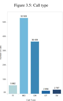
Figure 3.5: Call type
A call can be labeled in one of five groups:
• Fixed (FI) - the other person on that call belongs to a landline.
2
• Mobile (MO) - the other person on that call belongs to a mobile network. • On-Net (ON) - both ends of the call belong to WeDo operator.
4
• Services (SV) - voicemail, premium-rate, etc.
• Others (OT) - all the calls that do not belong to the previously mentioned groups.
6
Figure3.5shows the values dispersion regarding the type of the call. Around 90% of the calls belong to the Mobile and On-Net groups.
8
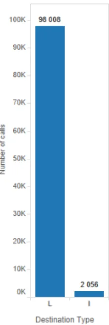
As shown in figure3.6, the majority of the calls are between numbers from the same country, named local (L) calls. Only 3% of the calls in our dataset are international (I).
Dataset
Figure 3.6: Call destination
A similar result can be found when analyzing dropped calls data. A call is said to be dropped when due to technical reasons, is cut off before the speaking parties had finished their conversation 2
and before one of them had hung up. On3.7we can see that a minority of our data has this specific
characteristic. 4
Dataset
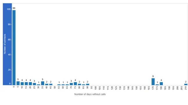
The main problem regarding our data was the lack of knowledge of what costumers churned and the ones that did not. According to some authors [Oentaryo et al., 2012,Radosavljevik et al., 2010],
2
we can state that a costumer has churned a telecom company when he does not do or receive any communication during 30 days or more.
4
The respective calculations were conducted, and final results are shown in figure3.8. More than 60 % of clients have done communications in less then 5 days, which tells they are currently
6
active. We also have an estimate of approximately 26% customers that churned the company, with a maximum day difference of 210 days without communications.
8
Figure 3.8: Days without calls
The final distribution of the clients concerning churn is represented in figure3.9. This is our target variable, which means that the objective of the developed models is to predict the outcome
10
of this variable through the study of the other variables in our data. We can already state that our target class is imbalanced, which means that the classes are not represented equally. This problem
12
Dataset
Dataset
3.4
Data transformation
Some algorithms in data mining require the dataset to have specific characteristics. The first step in
2
data transformation was to convert data types to most adequate ones. In figure3.10is represented the new data structure after this conversion. Most of the variables were converted to numeric type
4
to make the dataset easily adaptable to multiple algorithms. The exception in this conversion was the variable "churned" previously mentioned on section3.3. These variables were defined as a
6
factor. Factor variables are categorical variables that can be either numeric or string. Figure 3.10: Data structure after type conversion
Figure 3.11: Summary of new data
By the analysis of figure 3.11, we can clearly detect that there are big differences among
8
the variable ranges. Values for duration feature range between 1-7132, and values for msisdn feature range from 244575-31232100. This kind of variation could impact prediction accuracy
Dataset
[C.Saranya, 2013]. The objective is to improve predictive accuracy and not allow a particular
Chapter 4
Implementation and Results
2Regarding the models development, tunning and comparison, we chose R language [Foundation,] to implement and conclude the previously mentioned tasks. R is a language and environment for
4
statistical computing and graphics. It provides a wide variety of statistical and graphical tech-niques, and is highly extensible. The R installation already provides a software environment, but
6
we chose to use RStudio [R Core Team, 2013] as our integrated development environment (IDE). When compared with the built-in version, it provides additional features considered to be relevant
8
to the improvement of the development process.
4.1
Experimental Setup
10
To guarantee the results integrity when comparing multiple algorithms, we need to assure that all the algorithms are tested in the same conditions and with the same data mentioned on section
12
3.4. As the original data was ordered, we applied a randomize function to the dataset. We also removed variables "contract_id" and "msisdn" from the data that was going to train the multiple
14
models, because they have a direct connection with the outcome of target variable (identify the client itself).
16
The solution found consists in dividing the original data into two subsets: train set and test set with a 70/30 ratio.
18
The train set is formed by 70% of the original data, and aims to train the algorithm.
The test set contains 30% of the initial dataset, and is used to minimize overfitting and to tune
20
the algorithms parameters.
Has we have already mentioned on the previous section, our target class is imbalanced, and
22
this value disparity could have a significant negative impact on the final models regarding model fitting. Three main sampling methods were studied to solve this issue:
24
• Down-sampling • Up-sampling
26
Implementation and Results
The first method consists on randomly dividing all the classes items in the training set so that
their frequencies match the least common class. 2
The act of up-sampling data consists on randomly sampling the class with the lowest frequency
to be the same size as the majority class. 4
Hybrid methods can be considered middle ground of the previously mentioned techniques. This methods down-sample the majority class (churned) and synthesize new data points in the 6
minority class (not churned).
The chosen approach was a hybrid sampling method [Chawla et al., 2002] named Synthetic 8
Minority Over-sampling Technique (SMOTE) that was applied to the training set. This method approaches the data in two ways: generates new examples of the minority class using the nearest 10
neighbors of that cases, and under-samples the majority class.
In table4.1are the results of the applied sampling method. The first row of that table corre- 12
sponds to the dataset before the sampling method, and the second row to the data generated by
SMOTE method. 14
Table 4.1: Dataset Sampling results
Churn Churn % Not Churn Not Churn % Total
Original 18195 18,2 81869 81.8 100064
SMOTE 38211 42.9 50948 57.1 89159
The evaluation metrics chosen are Area Under Curve (AUC), sensitivity and specificity. The first approach was to use accuracy as a metric to evaluate the models, but due to the unbalancing 16
target class, where there was a low percentage of samples in one of the classes as mentioned on figure3.9, it was not good metric to be applied to our models. Next we present a brief description 18
of the evaluation metrics used:
• Specificity: Also called true negative rate, corresponds to the number of churned cases cor- 20
rectly identified divided by the total number of negatives (all the churn cases). Essentially, specificity represents the percentage of correctly classified cases when a costumer has not 22
churned.
• Sensitivity: Also known as true positive rate, measures the proportion between positive 24
examples which were predicted as positive. In our case, sensitivity means the percentage of
detected cases when a costumer has actually churned. 26
• AUC: A Receiver Operating Characteristic (ROC) chart is a curve representation of the proportion of false positives (1- specificity) on the horizontal axis against the proportion 28
of true positives on the vertical axis (sensitivity). This graph can be used to determine the optimal balance between sensitivity and specificity. AUC is a measure used to compare 30
accuracies of multiple classifiers and to evaluate how well a method classifies. The closer to 1 the AUC of a classifier is, the higher accuracy the method has. 32
Implementation and Results
In customer churn analysis it might be more expensive to incorrectly infer that customer is not churning then to give a general reduction in prices for services to clients that are not planning to
2
leave the company. Since the priority in our case study is given to identifying churn clients rather than not churn ones, Sensitivity is more relevant than Specificity in our results.
4
The algorithms applied were chosen due to their diversity of representation and learning style, and their common application on this kind of problems. We also took into consideration studies
6
regarding the popularity and efficiency [Wu et al., 2008].
Six different machine learning models were trained and compared among themselves. Those
8 algorithms were: • Knn 10 • Naive Bayes • Random Forest 12 • C4.5 • AdaBoost 14 • Ann
All the models were trained using functions available on R’s package caret[CRAN,], which
16
contains "functions for training and plotting classification and regression models".
Each model was tuned and evaluated using 3 repeats of 10-fold cross validation, a common
18
configuration on data mining for comparing different models [Kuhn, 2008]. The model with the best scores is then chosen to make predictions in new data, defined as test set.
20
A random number seed is defined before the train of each one of the algorithms to ensure that they all get the same data partitions and repeats.
22
The training of the models was done using the same data and control metrics, to establish a solid base for the future model comparisons. After the training phase, we made statistical
state-24
ments about their individual results and performance differences. All the resampling results were collected to a list using resamples() function, which checks that the models are comparable and
26
that they used the same training scheme (trainControl configuration). It also contains the evalu-ation metrics for each fold and each repeat per algorithm. The results and deep analysis of the
28
algorithms results will be presented on the next section.
All the computation during this research was done with the resources at FEUP Grid [FEUP,],
30
Implementation and Results
4.2
Results
In order to acquire the most adequate model to our problem, there is a need to explore which are 2
the best parameters for each algorithm. To do so, we constructed graphs with the performances of different algorithm parameter combinations, with the final objective of finding trends and the 4
sensitivity of the models.
The models were trained using 89159 entries, 10 predictors and 2 classes. 6
4.2.1 Knn
KNN is an extremely popular algorithm in classification that stores all available cases and clas- 8
sifies new cases based on a similarity measure to the previously saved ones. As we chose to use Euclidean distance as distance metric, the data was scaled between 0 and 1. The best choice of k 10
depends of the data: in most cases, larger values of k reduce the effect of noise on the classifica-tion, but make boundaries between classes less distinct [Everitt et al., 2011]. We studied the effect 12
of parameter k variation in the ROC and Sensitivity results, with the final objective of selecting the
one who reached the highest scores on those metrics. 14
The results of the train function are displayed bellow. With the analysis of these values we can infer that both the ROC and Sensitivity values are higher the algorithm takes into consideration 7 16
neighbors to decide. 18 1 k-Nearest Neighbors 2 20 3 89159 samples 4 10 predictor 22
5 2 classes: ’churned’, ’notchurned’
6 24
7 No pre-processing
8 Resampling: Cross-Validated (10 fold, repeated 3 times) 26
9 Summary of sample sizes: 80243, 80244, 80243, 80243, 80243, 80243, ...
10 Resampling results across tuning parameters: 28
11
12 k ROC Sens Spec 30
13 5 0.9549515 0.8817442 0.8904896
14 7 0.9498729 0.8693831 0.8769660 32
15 9 0.9440586 0.8577111 0.8658240
16 34
17 ROC was used to select the optimal model using the largest value.
18 The final value used for the model was k = 5. 36
On figure 4.1 the same results from the previous analysis are displayed. The graph shows 38
the number of neighbors on the x axis and ROC values on the y axis. We can conclude that 5 is the number of neighbors that give the best ROC and Sensitivity results, and that value keeps 40
Implementation and Results
Figure 4.1: Knn ROC value per number of neighbors
The training set class distribution was the following: • churned: 38211
2
• not churned: 50948
After this step, new predictions were conducted using new data (test set) that was not used to
4
train the model.
Using the knowledge acquired from the previous exploration, we chose 5 as the number of
6
neighbors to create the final classification model.
A confusion matrix was then created based on the algorithm predictions with the new data.
8
That confusion confusion matrix and associated statistics are listed bellow.
10
1 Confusion Matrix and Statistics
2
12
3 Reference
4 Prediction churned notchurned
14 5 churned 4263 3295 6 notchurned 1195 21265 16 7 8 Accuracy : 0.8504 18 9 95% CI : (0.8463, 0.8544) 1020 No Information Rate : 0.8182
11 P-Value [Acc > NIR] : < 2.2e-16
1222
13 Kappa : 0.5627
1424 Mcnemar’s Test P-Value : < 2.2e-16
15
1626 Sensitivity : 0.7811
17 Specificity : 0.8658
1828 Pos Pred Value : 0.5640
19 Neg Pred Value : 0.9468
2030 Prevalence : 0.1818
Implementation and Results
22 Detection Prevalence : 0.2518
23 Balanced Accuracy : 0.8234 2
24
25 ’Positive’ Class : churned 4
Although we accomplished a high Specificity value, the Sensitivity value was considerably 6
lower. And as already explained on section4.1, Sensitivity has more relevance to our model.
We also acquired the ROC curve of this model, in order to obtain our second metric AUC. The 8
ROC curve of this model is shown on figure4.2. The AUC of this model was 0.8883. Figure 4.2: Knn model ROC curve
Implementation and Results
4.2.2 Naive Bayes
Naive Bayes assumes that the value of a particular feature is independent from the value of any
2
other feature, given the class variable.
Regarding this algorithm a study was conducted around the influence of the kernel choice in
4
the models behavior.
When the "use kernel" value is set as TRUE, a kernel density estimate is used for density
6
estimation; if it is set as FALSE a normal density is estimated. The results of the this study are displayed bellow.
8 1 Naive Bayes 10 2 3 89159 samples 12 4 10 predictor
5 2 classes: ’churned’, ’notchurned’
14
6
7 No pre-processing
16
8 Resampling: Cross-Validated (10 fold, repeated 3 times)
9 Summary of sample sizes: 80243, 80244, 80243, 80243, 80243, 80243, ...
18
10 Resampling results across tuning parameters:
1120
12 usekernel ROC Sens Spec
1322 FALSE 0.6197166 0.6788183 0.4967745
14 TRUE 0.7035849 0.5686231 0.7421816
1524
16 Tuning parameter ’fL’ was held constant at a value of 0
1726 Tuning parameter ’adjust’ was
18 held constant at a value of 1
1928 ROC was used to select the optimal model using the largest value.
20 The final values used for the model were fL = 0, usekernel = TRUE and adjust = 1.
30
As we can deduce from the above results, the ROC value greatly increase when the option "usekernel" is activated, but the Sensitivity value decreases. We chose to keep the "usekernel"
32
option as TRUE as this algorithms best model.
Using the values which gave the best results in the previous experiment, we conducted new
34
predictions with that model on new data. In this way, we can truly evaluate the model behavior when tested with new values.
36
The confusion matrix values were:
38
1 Confusion Matrix and Statistics
2
40
3 Reference
4 Prediction churned notchurned
42
5 churned 3143 6173
6 notchurned 2315 18387
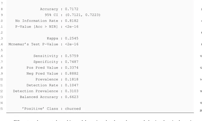
Implementation and Results
7
8 Accuracy : 0.7172 2
9 95% CI : (0.7121, 0.7223)
10 No Information Rate : 0.8182 4
11 P-Value [Acc > NIR] : <2e-16
12 6
13 Kappa : 0.2545
14 Mcnemar’s Test P-Value : <2e-16 8
15
16 Sensitivity : 0.5759 10
17 Specificity : 0.7487
18 Pos Pred Value : 0.3374 12
19 Neg Pred Value : 0.8882
20 Prevalence : 0.1818 14
21 Detection Rate : 0.1047
22 Detection Prevalence : 0.3103 16
23 Balanced Accuracy : 0.6623
24 18
25 ’Positive’ Class : churned
20
When tested on test data, this model continued to have the same behavior than in the train data: the Specificity value was extremely low, meaning that a lot of the clients who churned were 22
not identified as such. This could have a negative impact on the company economy, and does not fulfill the requirements established in the beginning of this process. 24
The ROC curve on figure4.3shows that we obtain an AUC value of 0.7092 in the Naive Bayes
model. 26