Blade pitch control malfunction simulation in a wind energy conversion system with MPC five-level converter

(1)

M. Seixas

abc

, R. Melício

ab

*, V.M.F. Mendes

bc

*, C. Couto

d

a_{IDMEC/LAETA, Instituto Superior Técnico, Universidade de Lisboa, Lisbon, Portugal} b_{Departmento de Física, Escola de Ciências e Tecnologia, Universidade de Évora, Évora, Portugal} c

Department of Electrical Engineering and Automation, Instituto Superior de Engenharia de Lisboa, Lisbon, Portugal d_{Centro Algoritmi, Universidade do Minho, Guimarães, Portugal}

Abstract

This paper is on a wind energy conversion system simulation of a transient analysis due to a blade pitch control malfunction. The aim of the transient analysis is the study of the behavior of a back-to-back multiple point clamped five-level full-power converter implemented in a wind energy conversion system equipped with a permanent magnet synchronous generator. An alternate current link connects the system to the grid. The drive train is modeled by a three-mass model in order to simulate the dynamic effect of the wind on the tower. The control strategy is based on fractional-order control. Unbalance voltages in the DC-link capacitors are lessen due to the control strategy, balancing the capacitor banks voltages by a selection of the output voltage vectors. Simulation studies are carried out to evaluate not only the system behavior, but also the quality of the energy injected into the electric grid.

Keywords: Wind energy; five-level power converter; drive train; fractional-order control; simulation.

1. Introduction

Environmental problems such as global warming and habitat preservation have to be faced by the society in nowadays in order to achieve a sustainable development. One of the causes for the global warming is said to be the increase on the level of CO2 in the atmosphere due to fossil fuel burning [1]. However, nowadays fossil fuel burning is needed for supplying the majority of the energy demand [2]. Research and development is on the way to achieve lower pollutants emissions on conversion of energy to convenient forms of usage in order to achieve a sustainable development. Conversion of energy from renewable energy sources are in nowadays a political attractive option [3] and a wind energy conversion system (WECS) is an economically viable exploitation [4], experiencing a significant expansion [5,6]. Although, onshore WECS deployments are cheaper than offshore ones, new suitable available onshore sites for deployments are becoming scarce, particularly in Europe [7]. So, the offshore WECS is becoming a further attractive option.

*Corresponding authors. Tel.: +351 266 745372; fax: +351 266 745394. E-mail address: ruimelicio@gmail.com (R. Melicio).

E-mail address: vfmendes@deea.isel.pt (V.M.F. Mendes).

Blade pitch control malfunction simulation in a wind energy

conversion system with MPC five-level converter

(2)

Nomenclature

u Wind speed value subject to the perturbation.

0

u Average wind speed.

n Kind of the mechanical eigenswing excited in the rotation wind turbine.

n

A Magnitude of the eigenswing n .

n

 Eigenswing frequency of the eigenswing n .

t

P Mechanical power on wind turbine.

tt

P Mechanical power on wind turbine disturbed by the mechanical eigenswings.

m Harmonic of the eigenswing.

nm

a Normalized magnitude of gnm.

nm

g Distribution of the harmonics in the eigenswing n .

n

h Modulation of the eigenswing n .

nm

 Phase of the harmonic m in the eigenswing n .

p

c Power coefficient.

 Tip speed ratio.

 Pitch angle of the rotor blades.

f b

P Mechanical power on wind turbine flexible blade part.

rb

P Mechanical power on wind turbine rigid blade part.

 Air density.

R Radius of the area covered by the blades.

r Radius of the area covered by the rigid blades part. t

 Rotor angular speed at flexible blades part.

b

J Moment of the inertia at the flexible blades part.

t

T

Mechanical torque.

db

(3)

bs

T Resistant shaft stiffness torque between the flexible blades part and hub.

h

 Rotor angular speed, at the hub plus rigid blades part.

h

J Moment of the inertia of the hub plus rigid blades part.

th

T Mechanical torque on rigid blades part.

dh

T Hub bearing resistant torque.

gs

T Shaft stiffness torque, between hub and generator.

g

 Rotor angular speed at the generator.

g

J Moment of inertia of the generator.

dg

T Generator bearing resistant torque.

g

T Electric torque.

sk

u Converter voltage.

mk

u Converter arm voltage.

cj

U Voltage at the capacitor bank j.

cj

i Current at the capacitor bank j.

dc

U Total DC voltage at the capacitor banks.

j

C Capacitance of the capacitor banks.

f k

i Currents injected into the electric grid.

n

L Inductance of the electric grid.

n

R Resistance of the electric grid.

f k

u Voltage at the filter.

k

u Voltage at the electric grid.

 Fractional order of the derivative or of the integral.

) (

 Real part of .

(4)

) (t

f Output of the controller.

p

K Controller proportional constant.

i

K Controller integral constant.



e Error on the stator electric current in the  plane.

 Error allowed for the sliding surface S(e_,t).



 Voltage output, hysteresis comparators,  plane.

H

X Root mean square value of the signal.

F

X Root mean square value of the fundamental component.

) (k

X Harmonic behaviour computed by DFT.

) (n

x Amplitude and phase of an input signal.

Energy policy is showing a shift towards favoring the offshore WECS, taking advantage of vast appropriated areas for possible deployment. Research and exploitation of floating oil platforms are important past work to the development of platforms for offshore wind energy exploitation [8]. For instance, a platform can be supported by a tripod ballast tank semi-submersible floating platform anchored to the sea bed by suspension tensioned steel cables. Also, wind speed are reported as tending to be considerably better and less variable on offshore than on onshore [7,9].

As stated in [10], the offshore WECS is stabilized by the action of a control in order to keep the floating platform with the less possible oscillations. The tripod ballast tank provides buoyancy to support the turbine and stability from the water plane inertia [11]. This configuration is a possible one, i.e., this configuration is not to be considered as a standard configuration. Actually as stated in [12], floating offshore wind turbines have no specific standards. The type of power transmission technology for offshore depends on the distance from the floating platforms to onshore: for shorter distances, below 60 km alternate current (AC) are reported as a favorable option, but for longer distances direct current (DC) is required [13]. The transmission might become too expensive [14] for faraway exploitation from shore. So, the use of near shore wind farms is the generally deployment.

(5)

The cost of repairing an outage on offshore is significantly greater and the condition for human intervention is not as feasible as in onshore. So, further attention has to be paid to eventual consequences of possible malfunctions in order to avoid outages. As wind energy is increasingly integrated into power systems the electric grid stability and power quality may be threatened [15]. The stability threaten is due not only to the intermittence and variability of wind energy, but also to malfunctions on the power electronic parts of the WECS, leading to a non anticipated shutdown. For instance, as the blade pitch control malfunction simulated in this paper. The power quality threaten is due to the injection of significant values of higher harmonics of current into the grid, leading to overvoltage in the grid or undesired performance on appliances of customers or both. So, simulation studies are important contributions in order to anticipate undesired impacts not only in the stability, but also the in the power quality [16]. Wind turbine operation at variable speed is a convenient option, because of the characteristics to achieve better efficiency at all operational range of wind speeds [17], allowing to improve energy capturing and to reduce the total harmonic distortion (THD) [18]. The technology for wind turbine operation at variable speed based on the use of permanent magnet synchronous generator (PMSG) as an option to conventional synchronous generators has the advantage of higher efficiency, due to null copper losses in the rotor [19] and the exclusion of the gearbox, due to ability to operate at low speed [20]. The exclusion of the gearbox mitigates not only the weight and the dimensions of nacelle equipment, but also the mechanic power losses in the conversion and maintenance requirements [19–21], which are of particular relevance for offshore deployment. The wind turbine can be operated at the maximum power operating point for various wind speeds by adjusting the shaft speed trough blade pitch control. Blade pitch control has become the dominating [22] strategy to achieve this operating point, due to the characteristic to move blades by varying the blade pitch angle according to the wind speed [23]. The behavior of the blade pitching system in blade pitch controlled wind turbines influences the overall dynamics [24,25]. So, research should be conducted to anticipate the possible repercussions during different abnormal operating conditions, such as a blade pitch control malfunction. A variable speed wind turbine having a PMSG needs an electronic full-power converter to convert the electric energy from a non-constant frequency into a constant one to be injected into an electric grid [18]. So, power converters are extremely important for the operation at variable speed [13]. Better power quality waveform [26], decreasing of THD [27], is possible by the increase on the number of voltage levels on the power

(6)

converter. Also, this increase allows for a reduction of the voltage on the insulated gate bipolar transistors (IGBTs). So, the five-level converter is expected to be a promising option in power systems. Malfunctions occurring on the control in WECS have to be conveniently accounted to mitigate unavailability in order to achieve condition for recovering the convenient operation. A five-level converter is a favorable option for this mitigation: the higher number of capacitors banks storing energy allows mitigation of unavailability. However, five-level converters have drawbacks: voltage unbalances, high component count, and increased control complexity. A critical issue in five-level converters is the control of the unbalance voltage on the capacitors.

The WECS is equipped with a PMSG using a back-to-back multiple point clamped (MPC) five-level converter topology, using unidirectional commanded IGBTs, converting the energy of a variable frequency source in an appropriated form with constant frequency to be injected into the electric grid through an AC link. The drive train considered is described by a three-mass model. Additionally, a fractional-order control strategy on the PMSG/full-power converter topology is considered. In this paper the focus is on a transient analysis of the MPC five-level converter performance of the WECS due to a blade pitch control malfunction. This malfunction imposes an instantaneous cut-off on the capture of the energy from the wind by the blades. This is the worst case in what regards the capability of the MPC five-level converter to ensure as much as necessary condition for maintaining the interconnection with the grid. Previous work on blade pitch control malfunction is mainly focused on onshore exploitation of wind power implemented with two-level or three-level converters [28]. Not enough attention has been given to the simulation of five-level converters. So, the present study is a contribution for the state of art of blade pitch control malfunction assessment on a five-level converter by a simulation study of the blade pitch control malfunction. The rest of this paper is organized as follows. Section 2 presents the modeling for the WECS. Section 3 presents the control strategy. Section 4 presents the case study. Finally, concluding remarks are given in Section 5.

2. Modeling

(7)

The model for wind speed reported in [29] is used in this paper. The WECS is considered to be subjected to the variation in wind speed. This variation is responsible to produce undesired perturbation on the mechanical torque. This research is important to unveil the influence on the injected electrical current in what regards the harmonic distortion.

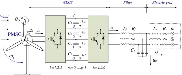
The implementation of the back-to-back MPC five-level power converter into the configuration of the simulated WECS is shown in Fig. 1.

k=1,2,3 nk=0,…,p-1 k=4,5,6 C3 C2 C1 ic3 1 2 3

PMSG

i

k t



2



L

f

R

f

L

n

R

n

C

f Electric grid

i

fk

u

fk

u

k 0 WECS Filter

i

k ic2 ic1 Wind C4 ic4 4

Fig. 1. WECS equipped with five-level power converter.

2.2 Wind Speed

Although the wind speed has a stochastic behavior, for the type of simulation purpose and for the type of wind turbine studied in this paper is normally admissible to model the wind speed as a sum of harmonics with the frequency range 0.1–10 Hz [30] given by:



  n n n t A u u ₀[1 sin( )] (1) 2.3 Wind Turbine

The conversion of wind energy into mechanical energy is influenced by various forces acting on the wind turbine blades and tower, deriving not only the desired mechanical power, but also the unavoidable mechanical perturbation. This mechanical perturbation is modeled by eigenswings, considering three

(8)

influences of the dynamic associated with the action excited by wind on the physical structure: I1 the

asymmetry in the turbine, I2 the vortex tower interaction and I3 the eigenswings in the blades [29,33].

The dynamic associated with the asymmetry in the turbine is assessed considering the following data:A₁0.01

,

a₁₁4/5

,

a₁₂1/5

,

₁(t)_t(t)

,

₁₁0

,

and ₁₂/2

.

The dynamic associated with the vortex tower interaction is assessed considering the following data: A₂0.08,

2 / 1

21

a , a₂₂ 1/2, ₂(t)3_t(t), ₂₁0, and ₂₂/2. The dynamic associated with the eigenswings in the blades is assessed considering the following data: A30.15, a311,

] ) ( ) ( [ 2 / 1 ) ( ₁₁ ₂₁ 3 t  g t g t

 , and ₃₁0. The mechanical power of the wind turbine, disturbed by the dynamic influences is given by:

] ) ( ) ) ( ( 1 [ 3 1 2 1

 

    n n m nm nm n tt t P A a g t h t P (2) where ) ' ) ' ( ( sin 0



  t _n _nm nm m t dt g   (3)

The determination of the power coefficient cp involves the use of blade element theory and the

knowledge of blade geometry. These complex issues are normally treated by numerical approximation as the one developed in [34] and followed in this paper. The power coefficient is given by:

i i p e c     4 . 18 2 . 13 002 . 0 58 . 0 151 73 . 0 2.14            (4) where ) 1 ( 003 . 0 ) 02 . 0 ( 1 1 3_       _i (5)

A non-linear mathematical programming problem with the objective function (4) and subjected to (5) at a null blade pitch angle is used to compute the global maximum and the optimal tip speed ratio, having respectively, the values given by:

4412 . 0 (0),0] [ max opt  p c 

_opt(0)7.057 (6)

(9)

The algorithm of maximum power point tracking (MPPT) is one of the main procedures used to effectively capture wind energy [35] by the conversion system. But, gusts generated impact on the drive train and contribute significantly to fatigue loading due to rapid shaft torsional torque variations. Hence, a trade-off between optimum power coefficient operation and avoidance of rapid shaft torsional torque variations is important in practical implementations for reducing fatigue stresses [36]. But, a transient analysis for wind turbines equipped with a PMSG during a blade pitch control malfunction can be performed with only the MPPT in order to avoid unnecessary modeling of the trade-off as in [37]. The simulation of the blade pitch control malfunction considers that the blade pitch angle control imposes the position of wind gust on the blades in a small time interval, i.e., blades are quickly at the position of the maximum blade pitch angle. The minimum power coefficient and the associated tip speed ratio are respectively [28] given by:

0025 . 0 min  p c

_min 3.475 (7)

The values in (7) are for the blade pitch angle _max55º.

2.4 Drive Train Model

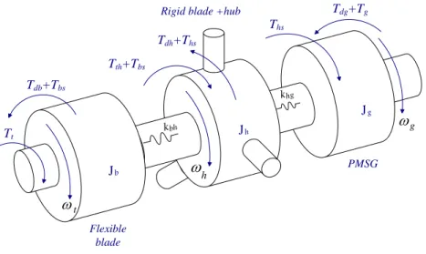
The increase in power of the wind turbines implies that the blades are larger, more flexible and tend to bend. One way to determine the dynamic properties of the blades is through the use of finite element methods, but this approach cannot be straightforwardly accommodated in the context of studies of power system analysis [38,39]. Thus, to avoid the use of finite element methods, the drive train dynamics is simplified and represented as a torsion system with discretization of masses. The discretization of mass is given by a three-mass model, having as input the mechanical torque due to the effect of the wind. The blade bending occurs at a significant distance from the joint between the blades and the hub [40], so the blades are model as consisting in two segments: a flexible one and a rigid one. Also, for transient stability analysis, the generator is described by one mass associated with the mechanical inertia of the generator rotor in order to capture the effect of the mechanical perturbation on the electrical harmonic distortion. Therefore, the drive train is modeled by three coupled inertial masses as shown in Fig. 2.

(10)

Jb Jg Tt Tth+Tbs Tdb+Tbs Jh Flexible blade

Rigid blade +hub

PMSG Ths Tdh+Ths Tdg+Tg kbh khg g  t  h



Fig. 2. Drive train model.

Fig. 2 shows: the flexible blade mass concentrating the inertia of the flexible segment of the blades; the rigid blades +hub mass concentrating the inertia of the rigid segment of the blades and the hub; the PMSG mass concentrating the inertia of the generator. The equations for the three-mass model are based on the torsional version of the second law of Newton [32]. The state equations for the three-mass model are respectively given by:

) ( 1 bs db t b t _T _T _T J dt d     (8) ) ( 1 hs dh bs th h h _T _T _T _T J dt d      (9) ) ( 1 g dg hs g g T T T J dt d     (10)

The wind turbine mechanical power P_tt over the rotor, considering the flexible and rigid segments of the blades in the drive train, is given by:

rb fb tt P P P   (11) where p fb R r u c P ( 2 2) 3 2 1 _   (12) p rb r u c P 2 3 2 1__  (13)

(11)

2.5 Generator

The generator considered in this paper is a PMSG. The equations for modeling a PMSG can be found in literature [41,42]. In order to avoid demagnetization of permanent magnet in the PMSG, a null reference stator direct component current i_sd* 0 is imposed [43].

2.6 Five-Level Power Converter

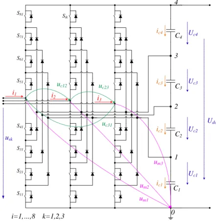
The back-to-back MPC five-level power converter is an AC-DC-AC power converter, equipped with twenty four unidirectional commanded IGBTs implementing the rectifier. More detail of the rectifier for the five-level power converter is shown in Fig. 3.

usk C1 C2 C4 Udc Uc4 Uc2 Uc1 0 1 3 i3 i=1,…,8 k=1,2,3 um1 um2 um3 ic1 ic2 S81 S71 S51 S41 S31 S11 i2 i1 uc23 uc12 uc31 ic4 S61 S21 C3 Uc3 2 ic3 4 Sik

Fig. 3. Five-level power rectifier converter.

Fig. 3 shows the IGBT identified by Sik. The same number of unidirectional commanded IGBTs identified by the same notation, but with convenient particularization for the second index, implements

(12)

the inverter. The index i with i{1, ..., 8} identifies the IGBT. The index k with k{1,2,3} identifies the leg for the rectifier and k{4,5,6} identifies the leg for inverter. The groups of height IGBTs linked to the same phase constitute the leg k of the converter. The five valid conditions [33,44] to be applied for the switching voltage level variable of each leg k and at each level are given by:

              nd S nd S S S nd S nd S S S nd S nd S S S nd S nd S S S nd S nd S S S n k k k k k k k k k k k k k k k k k k k k k a 1 ) a , , ( , 0 a 1 ) a , , ( , 1 a 1 ) a , , ( , 2 a 1 ) a , , ( , 3 a 1 ) a , , ( , 4 4 3 2 1 5 4 3 2 6 5 4 3 7 6 5 4 8 7 6 5             0 ) a , , ( 0 ) a , , ( 0 ) a , , ( 0 ) a , , ( 0 ) a , , ( 8 7 6 5 8 7 6 1 8 7 2 1 8 3 2 1 4 3 2 1 k k k k k k k k k k k k k k k k k k k k S nd S S S S nd S S S S nd S S S S nd S S S S nd S S S

k{1,...,6} (14)

The switching states combinations, identifying the conduction or the blockage state of the IGBTs of each leg k, determine the level variable

k jn

 that is associated with the charging state of each capacitor

bank. The level variable [45] is given by:

      k k jn _j _n n j k ₁ 0 

j{1,...,p1}

,

n_k{0,..., p1} (15)

Thus, the capacitor bank C4 charging state is only changed if at least one of the legs k presents a combination of IGBTs switching states that select the switching variable of the leg k at level 4, i.e.,

4 

k

n . The capacitor bank C3 changes the charging state as long as one leg presents a combination of

IGBTs switching states that select level 4 or level 3. The capacitor bank C2 changes the charging state as

long as one leg presents a combination of IGBTs switching states that select level 4 or level 3 or level 2. The capacitor bank C1 changes the charging state as long as one leg presents a combination of IGBTs

switching states imposing the selection of level 4, level 3, level 2 or level 1. If the level imposed by the selection is n_k 0, then no capacitor charging state is affected.

The rectifier is connected between the PMSG and a capacitor banks. The inverter is connected between this capacitor banks and a second order filter, which in turn is connected to an electric grid. The switch delays, dead times, on-state semiconductor voltage drops and snubber networks are disregarded [46].

The modeling for the rectifier considers the line voltage ucab as a function of the leg voltage usk or

mk u given by: mb ma sb sa cab u u u u u    

a,b{1,2,3} for ab (16)

(13)

The difference of voltages between the lines as a function of u_sk or u_mk for ab,ak,bk are given by:



         3 1 3 1 2 2 k a a ma mk k a a sa sk cbk cka u u u u u u k,a{1,2,3} (17)

A balanced three phase electrical generator imposes the condition given by:

0 3 1 



 k sk u k{1,2,3} (18)

From (17) and (18) the voltages differences between the lines are given by:

sk ckb

cka u u

u  3 k,a{1,2,3} (19)

From (18) and (19) holds the relation given by:



    3 , 1 2 3 k a a ma mk sk u u u k,a{1,2,3} (20)

The leg voltage umk as a function of jn_k and the capacitor banks voltage Ucj for jnk {0,1} and

} 3 , 2 , 1 {  k given by:



   1 1 p j cj jn mk U u k  j{1,...,p1}, n_k{0,..., p1} (21)

From (19)–(20) the rectifier input voltage usk as a function of jn_k for j{1,...,p1}, } 1 , ... , 0 {   p n_k and {0,1} k jn  is given by:







     1 1 3 , 1 ) 2 ( 3 1p j cj k l l jn jn sk U u l k   k{1,2,3} (22)

The modeling applied to the inverter is similar to the one of the rectifier. Consequently, the inverter output voltage for j{1,...,p1}, n_k{0,..., p1} and _jn_k {0,1} is given by:







     1 1 6 , 4 ) 2 ( 3 1p j cj k l l jn jn sk U u l k   k{4,5,6} (23)

(14)

The current i on each capacitor bank cj C is associated with the level variable j jn_k , defining whether the input phase currents i in the rectifier or the output phase currents _k i of the inverter determines a _k

possible change to the charging state of the capacitor banks, according to the voltage level in the leg k. The current on each capacitor bank i as a function of _cj

k jn  for j{1,...,p1}, n_k{0,..., p1} and } 1 , 0 {  k jn  [47] is given by: k k nk k k nk cj i i i



    6 4 3 1   k{1,...,6} (24)

The charging state changes of the capacitor banks are obtained by the consideration of the electric circuit detail as shown in Fig. 4.

C1 C2 C3 j=3 ic1 ic2 ic3 j=2 j=1 j=0 C4 j=4 ic4 i1 i2 i3 i5 i4 i6

Fig. 4. . Capacitor banks current.

For instance, if the rectifier legs present the IGBT state combination of n₁3, n₂1 and n₃ 0, and the inverter legs present the IGBT state combination of n4 3, n54 and n6 2, the currents on the

capacitor banks are respectively given by:

5 6 4 4 3 1 4 4 i i i i k k n k k n C 



k 



k      (25)

(15)

5 4 1 6 4 3 3 1 3 3 i i i i i i k k n k k n C 



k 



k        (26) 6 5 4 1 6 4 2 3 1 2 2 i i i i i i i k k n k k n C 



k 



k         (27) 6 5 4 2 1 6 4 1 3 1 1 1 i i i i i i i i k k n k k n C 



k 



k          (28) The voltage U_dc is the sum of the capacitor voltages U_c₁, U_c₂, U_c₃, U_c₄ in the capacity banks C1,

2

C , C3, C4 modeled by the state equation given by:



   1 1 1 p j cj j dc _i C dt dU j{1,..., p1} (29)

2.6 Line and Filter

The line, Fig. 1 is connected between the inverter and the second order filter and is modeled by an inductance,Lline, in series with a resistance,Rline. The second-order filter is modeled by an

inductanceLfilter, a resistanceRfilter, and a capacitor Cf . The resistances and inductances of the line and

the filter are associated in an equivalent resistance and inductance [32], respectively given by:

       filter line f filter line f R R R L L L (30)

The inverter output phase currents are given by:

) ( 1 k f k f sk f k _u _R _i _u L dt di    k{4,5,6} (31)

The filter output voltage, i.e., at the electric grid connection point is given by:

) ( 1 k f k t f k f i i C dt du   k{4,5,6} (32)

(16)

2.7 Electric Grid

A three-phase active symmetrical circuit in series models the electric grid [32]. The current injected into the electric grid is modeled by the state equation given by:

) ( 1 k fk n fk n fk u i R u L dt di    k{4,5,6} (33)

This model assumes that the electric grid is represented by a short-circuit inductive impedance in series with an ideal sinusoidal voltage source.

3. Control Strategy

3.1 Fractional-Order Controllers

Fractional-order PI control is based on fractional calculus theory, which is a generalization of ordinary differentiation and integration to arbitrary order, i.e., the order is not necessarily an integer one

[48]. Fractional calculus theory are being used in mathematical models and have been proved as having handiness on the design, properties and controlling abilities in order to achieve a more convenient performance on dynamic systems [47].

The fractional-order derivative or integral can be denoted by a general operator _aD_t [49] given by:

              



 ( ) 0 0 ) ( 0 ) ( , ) ( , 1 ,         t a t a d dt d D (34)

where () is the real part of the , if ()0 then  is the order of the derivative or the integral, if

0 )

( 

 then - is the order of the integration. In (34) a and t are the limits of the integration, and 

(17)

Several approaches are possible for defining a fractional-order derivative and a fractional-order integral. The Riemann–Liouville definition is the most frequently reported as being in application. This definition is given by:



  _   t a t aD f t _ t   f  d  ) ( ) ( ) ( 1 ) ( 1 (35)

where Γ x( ) is the Euler’s Gamma function given by:



     0 1 ) (x yx e ydy (36)

Other approach is the Caputo definition for the fractional-order derivative given by:



_      t a n n t C a d t f n t f D       1 ) ( ) ( ) ( ) ( 1 ) ( (37)

Or the approach of Grünwald–Letnikov definition given by:



   _      h a t r t a f t rh r r h t f D h 0 ) ( ) ( ! ) ( lim ) ( 0     (38)

with the definition of fractional-order derivatives given by:

) ( ) 1 ( ! ) 1 ( ) 1 ( lim ) ( 0 0 h r t f r r h t f D h a t r r t a h        



        (39)

In this paper,  is a real number satisfying the restrictions 01. Also, a0 and the following notational convention 0Dt Dt are assumed.

The definition of Riemann–Liouville and Grünwald–Letnikov revealed an important property, while integer-order operators are defined by finite series, the fractional-order counterparts are defined by infinite series [47,49], which means that the integer operators are local operators in opposition with the fractional operators which implicitly have more memory of the past events. The fractional-order controller has the advantage of providing more criterion than the classical one, expanding the freedom for imposing an improved behavior [50]. The dynamic behavior of the fractional-order controller is described by a fractional differential integral equation with an integral or a derivative having at least a non-integer order. The differential equation of the fractional-order PI is given by:

(18)

) ( ) ( ) (t K et K D et f  _p  _i _t (40)

A classical PI controller is modeled by taking 1 in (40). The transfer function of the fractional-order PI using the Laplace transform on (40) is given by:

   K K s s G( ) _p _i (41)

The fractional-order PI controller has one more adjustable parameter, which reflects the intensity of integration making the fractional-order PI controller more flexible than the classical PI controller. Normally heuristic methods are reported for adjusting the parameters in order to achieve a convenient performance, for instance, as the heuristic method in [51] used in this paper. The design of PI controllers follows the tuning rules in [51].

3.2 Power Converter Control

The MPC five-level power converter has a variable structure behavior. This behavior is due to the conduction or the blockage of IGBT, i.e., on/off switching states. Pulse width modulation (PWM) by space vector modulation (SVM) associated with sliding mode (SM) is used for controlling the power converters. As mentioned previously, the controllers proposed for the power converter are fractional-order PI controllers. The difference between the voltage Udc and the reference voltage

*

dc

U is processed by the PI controller in order to determine a reference for the stator currents. The difference between the stator current and the reference stator current is used in the strategic selection envisaged for the output voltage vector in the (,) space.

The SM control presents attractive features such as robustness to parametric uncertainties of the wind turbine and the generator as well as to electrical grid perturbation [52,53]. The SM control is a method that adjusts the variable state of a system by applying a discontinuous control signal that forces the system onto a particular surface in the state space, named sliding surface S(e_,t). Once the sliding surface is reached, the sliding mode control maintains the system on a small neighborhood of the sliding surface. If the system drifts away, then the power converter state is subjected to a change in order to determine actions to bring the system back to the sliding surface. The SM control attractive features are important

(19)

for adjusting the power converter by ensuring the choice of the appropriate space vector which will trigger the IGBTs.

The IGBTs have physical limitations that have to be considered during not only design phase, but also on simulation studies. Particularly, the switching state of the IGBTs has to be made at a finite frequency. For instance, frequencies for the switching state of the IGBTs are reported to be in use as 2 kHz, 5 kHz or even 10 kHz. This IGBTs physical limitation implies that the control of the electric current will not be able to follow exactly the reference value and an error in the  plane,e, has to be accepted. The

system slides along the sliding surface,S(e,t), in order to assurance that that the state trajectory near the surface endorses the stability conditions [44,52] given by:

0 ) , ( ) , (  dt t e dS t e S _  (42)

A small error  0 for S(e,t) is allowed, due to IGBTs switching only at finite frequency. This error over time is the sliding surface. The switching strategy is given by:



  _ 

 S(e ,t) (43)

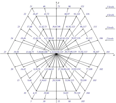
A practical implementation of the switching strategy considered in (43) for the simulation is accomplished by the use of hysteresis comparators. The outputs coming from the hysteresis comparators are the integer variables, giving the vector _ (_,_) [52]. For the five-level power converter, the output voltage vectors in the (,) space are shown in Fig. 5.

(20)

  2 levels 3 levels 4 levels 5 levels 21 46 71 96 121 5 30 55 80 105 61,92,123 23 111 16,47 41,72 66,97 91,122 22 116 29,60 54,85 79,110 10 104 3,34,65 78,109 9,40 15 103 11,42,73 36,67,98 2,33,64,95 8,39,70 27,58,89,120 77,108 14,45 20 52,83,114 102 28,59,90 53,84,115 4,35 17,48 86,117 6,37,68,99 12,43,74 31,62,93,124 81,112 18,49 24 56,87,118 106 7,38,69,100 13,44,75 1,32,63,94,125 76,107 19,50 25 26,57,88,119 51,82,113 101

Fig. 5. Output voltage vectors for the five-level power converter.

The integer voltage variables  and  have a discrete domain given by:

} 4 , 3 , 2 , 1 , 0 , 1 , 2 , 3 , 4 { , _         (44)

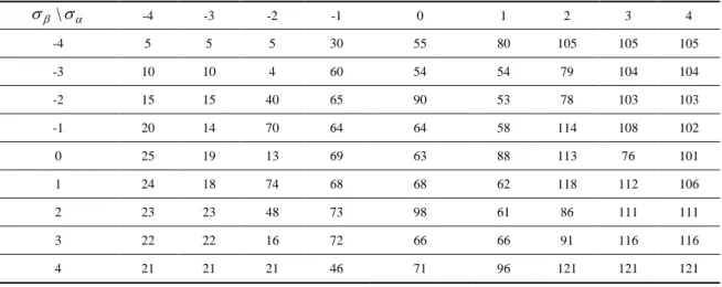
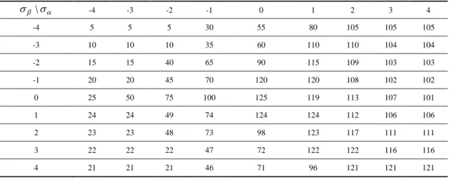
The variables  and  allow choosing the appropriate vector. On the inner output voltage vectors there are redundant ones corresponding to combinations of IGBT states, different from each other, corresponding to a different level selection. This control strategy is proposed to ensure performance of the five-level power converter and to mitigate the capacitors unbalancing voltages. Hence, the selection of the appropriate vector, taking into account both external and internal hexagons [40] formed by the output voltage vectors can be given by the following five tables: Table 1 summarizes the vector selection for

0

k

n  ; Table 2 summarizes the vector selection for n_k 1; Table 3 summarizes the vector selection for

2

k

n  ; Table 4 summarizes the vector selection for n_k 3; Table 5 summarizes the vector selection for

4

k

(21)

Table 1. Five-level power converter output voltage vectors selection for n_k 0     \ -4 -3 -2 -1 0 1 2 3 4 -4 5 5 5 30 55 80 105 105 105 -3 10 10 4 4 29 54 104 104 104 -2 15 15 9 3 28 53 78 103 103 -1 20 20 14 2 2 52 77 102 102 0 25 50 13 100 1 26 51 76 101 1 24 24 18 6 6 56 81 106 106 2 23 23 17 11 36 61 86 111 111 3 22 22 16 16 41 66 116 116 116 4 21 21 21 46 71 96 121 121 121

(22)

The control strategy for the WECS has a block diagram as shown in Fig. 6.

PMSG Lf Rf Cf ik ik uf45 uf56 uf64 456 dq udq + -μ PI * idq* dq αβ * iαβ -+ if456 456 αβ iαβ SVM SM SVM SM Udc + -μ PI idq* dq αβ 123 αβ iαβ iαβ* -+ i123 ifk -* g  g  g  k=1,2,3 nk=0,…,p-1 k=4,5,6 C3 C2 C1 ic3 1 2 3 0 ic2 ic1 C4 ic4 4 U_dc U_dc* Udc 123 n 123 jn  n456 456 jn 

(23)

Fig. 6 shows that the Fractional-order control is used for the variable-speed operation of wind turbine with the PMSG and for the five-level full-power converter in order to find the reference currents.

4. Case Study

The model for the WECS is implemented in Matlab/Simulink with a 6 s of time horizon for the simulation. The WECS has a rated electric power of 2 MW and the capacitor banks reference voltage

*

dc

U is 6 kV. The fractional controllers parameters are 0.5, K_i 2.6, as discussed in [51]. The air density is 1.225 kg/m3. The switching frequency for IGBTs is 10 kHz. The wind speed has an average speed of 14.5 m/s.

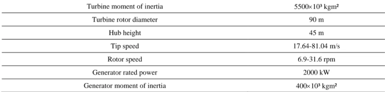
Table 6 summarizes the WECS data.

Table 6. WECS data

Turbine moment of inertia 550010³ kgm²

Turbine rotor diameter 90 m

Hub height 45 m

Tip speed 17.64-81.04 m/s

Rotor speed 6.9-31.6 rpm

Generator rated power 2000 kW

Generator moment of inertia 40010³ kgm²

The electric grid has 6 kV at 50 Hz. The wind speed data is: u₀ 14.5; A₁0.01, ₁(t)_t(t);

08 . 0

2

A , 2(t)3t(t), A30.15, 3(t)1/2[g11(t)g21(t)] with g11(t)and g21(t) given by

(3), i.e., the wind speed is given by:

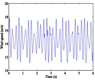
] ) ( sin 1 [ 5 . 14 3 1



   n n n t A u  0t6 (45)

(24)

Fig. 7. Wind speed profile.

The blade pitch control malfunction is assumed to occur between 2.0 s and 2.5 s, imposing a total instantaneous cut-off on the capture of the energy from the wind by the blades [28]. There is no capture of wind energy to help holding the electric connection with the electric grid. The rotor speed decreases smoothly due to the mechanical inertia. So, if the kinetic energy and the electric energy stored in the capacitor banks are not appropriated, the electric interconnection is in menace by the back-to-back MPC full-power five-level converter, i.e., the system recovery is in menace. This is the worst case due to the blade pitch control malfunction in what regards the behavior of a back-to-back MPC full-power five-level converter. The system is subjected to the worst case that has to be anticipated to mitigate unavailability in order to achieve condition for recovering the convenient operation.

The wind speed profile is showed in Fig. 7 and is numerical given by (45). The blade pitch angle behavior is shown in Fig. 8.

(25)

Fig. 8 shows that although blade pitch angle is imposed at the wind gust position during blade pitch control malfunction, after the malfunction the blade pitch angle recovers the behavior of a convenient operation in response to the wind energy available.

The power coefficient is shown in Fig. 9.

Fig. 9. Power coefficient.

Fig. 9 shows that although power coefficient is imposed as having the minimum value during blade pitch control malfunction, after the malfunction the power coefficient recovers the behavior for energy capturing in response to the wind energy available. Observe that this behavior is not only dependent of the behavior of the blade pitch angle shown in Fig. 8, but also of the tip speed ratio. So, the behavior of the tip speed ratio is also recovered.

The torques are shown in Fig. 10.

(26)

Fig. 10 shows that the flexible blade torque (blue) is null during blade pitch control malfunction, the rigid part of the blades plus hub torque (red) is in oscillation due to the elastic modeling of the interface between the masses. The electric torque (green) is the final torque action on the PMSG.

The rotor speed of the flexible blade (blue), the rotor angular speed of the rigid part of the blades plus hub (red) and the rotor angular speed of the generator (green) are shown in Fig. 11.

Fig. 11. Rotor speed of the flexible blade, rigid blade plus hub and generator.

Fig. 11 shows that although there is no energy captured from the wind energy during blade pitch control malfunction, the speed of the rotor during the malfunction is feasible. After the malfunction, the behavior of the kinetic energy stored in the rotor is recovered. The variations between the three speeds are due to the induced torsional effect forcing an elastic behavior on the rotor.

The voltage at the capacitor banks during the blade pitch control malfunction are shown in Fig. 12.

(27)

Fig. 12 shows that although pitch control malfunction occurs between 2.0 s and 2.5 s, the voltages at the capacitor banks are convenient hold to sustain the electric connection with the grid.

The instantaneous current injected into the electric grid is shown in Fig. 13.

a) b)

Fig. 13. Current injected in the electric grid.

Fig. 13 show: a) the effect of the malfunction in the current injected into the electric grid is recovered and is equivalent to a decrement on power captured from the wind; b) the instantaneous current injected into the electric grid is almost a three phase alternate sinusoidal current. Some perturbation occurs as can be revealed by the harmonic content of the current injected into the electrical grid given by the THD. The THD is given by:



  2 2 1 100 (%) THD H H F X X (46)

The harmonic content is computed by the Discrete Fourier Transform (DFT) given by:



    1 0 2 ) ( ) ( N n N n k j n x e k X  for k0,...,N1 (47)

(28)

Fig. 14. THD of the current injected into the electric grid.

The average THD of the current injected into the electric grid is 0.53%. Fig. 14 shows that the THD of the current injected into the electric grid is less than IEEE-519 standard 5% limit [54]. Hence, the five-level power converter is an interesting option in what regards the THD. Although IEEE-519 standard is not necessarily imposed on WECS is used in this paper as a guideline for the quality of energy injected into the electric grid.

5. Conclusions

Wind power penetration in electric grids leads to new technical challenges, concerning transient stability and power quality. A model and a simulation study are presented for WECS equipped with a permanent magnet synchronous generator and with a back-to-back multiple point clamped five-level power converter. The model takes into account wind perturbation. The simulation is intended to evaluate the WECS behavior when a blade pitch control malfunction occurs, imposing a total instantaneous cut-off on the capture of the energy from the wind by the blades. This malfunction subjects to the worst case the energy stored in the capacitor banks in what regards the achievement of condition for recovering the convenient operation.

The case study imposes a total instantaneous cut-off on the capture of the energy from the wind by the blades during 0.5 s. The simulation reveals that no outage is foreseen and a convenient performance, in what regards the effect on the current output of the power converter measured by the average value of the

(29)

THD, is achieved. The current injected into the electric grid is lower than 5% limit imposed by IEEE-519 standard [54]. The blade pitch control malfunction does not significantly echo on voltage dropping in the capacitor banks, contrary to what is reported in [28], where a three-level converter is used. The five-level power converter due to a high level of energy stored in the capacitor banks sustains the DC voltage.

This type of simulation is able to decide if the malfunction eventually leads to an outage, meaning that if the simulation is in favor of no outage, then no outage is expected to happen. The authors believe that for an offshore WECS, the marine wave perturbation may be treated as an augmented wind perturbation in what regards the study of the electrical behavior of an offshore WECS.

Acknowledgment

This work is funded by Portuguese Funds through the Foundation for Science and Technology-FCT under the project LAETA 2015‐2020, reference UID/EMS/50022/2013.

References

[1] M. Tahir, and N.S. Amin, "Advances in visible light responsive titanium oxide-based photocatalysts for CO2

conversion to hydrocarbon fuels," Energy Conversion and Management, vol. 76, pp. 194-214, 2013.

[2] F. Blaabjerg, R. Teodorescu, M. Liserre, and A.V. Timbus, "Overview of control and grid synchronization for distributed power generation systems," IEEE Transactions on Industrial Electronics, vol. 53, pp. 1398-1409, 2006.

[3] L.M.C. Ferro, L.M.C. Gato, and A.F.O. Falcão, "Design of the rotor blades of a mini hydraulic bulb-turbine," Renewable Energy, vol. 36, pp. 2395-2403, 2011.

[4] B.R. Sarker, and T.I. Faiz, "Minimizing maintenance cost for offshore wind turbines following multi-level opportunistic preventive strategy," Renewable Energy, vol. 85, pp. 104-113, 2016.

[5] J.K. Kaldellis, K. Garakis, and M. Kapsali "Noise impact assessment on the basis of onsite acoustic noise immission measurements for a representative wind farm," Renewable Energy, vol. 41, pp. 306-314, 2012. [6] S. Dong, S. Tao, X. Li, and C. Guedes Soares, "Trivariate maximum entropy distribution of significant wave

height, wind speed and relative direction," Renewable Energy, vol. 78, pp. 538-549, 2015.

[7] T. Soukissian, "Use of multi-parameter distributions for offshore wind speed modeling: the Johnson SB distribution," Applied Energy, vol. 111, pp. 982-1000, 2013.

[8] M. Esteban, and D. Leary, "Current developments and future prospects of offshore wind and ocean energy," Applied Energy, vol. 90, pp. 128-136, 2012.

[9] B. Lange, S. Larsen, J. Højstrup, and R. Barthelmie, "Importance of thermal effects and sea surface roughness for offshore wind resource assessment," Journal of Wind Engineering and Industrial Aerodynamics, vol. 92, pp. 959-988, 2004.

[10] D. Alvarenga, "Pilot floating wind power project seeks EU funds," Wind Float, (http://www.principlepowerinc.com/products/windfloat.html) 2012.

(30)

[11] E.E. Bachynski, M. Etemaddar, M. Kvittem, C. Luan, and T. Moan, "Dynamic analysis of floating wind turbines during pitch actuator fault, grid loss, and shutdown," Energy Procedia, vol. 35, pp. 210-222, 2013.

[12] D. Roddier, C. Cermelli, A. Aubault, and A. Weinstein, "A floating foundation for offshore wind turbines," Journal of Renewable and Sustainable Energy, vol. 2, pp. 033104-1-033104-34, 2010.

[13] J.M. Carrasco, L.G. Franquelo, J.T. Bialasiewicz, E. Galván, R.C.P. Guisado, M.A.M. Prats, J.I. León, and N. Moreno-Alfonso, "Power-electronic systems for the grid integration of renewable energy sources: a survey," IEEE Transactions on Industrial Electronics, vol. 53, pp. 1002-1016, 2006.

[14] J.I. Marvik, E.V. Øyslebø, and M. Korpås, "Electrification of offshore petroleum installations with offshore wind integration," Renewable Energy, vol. 50, pp. 558-564, 2013.

[15] J. Mohammadi, S. Afsharnia, and S. Vaez-Zadeh, "Efficient fault-ride-through control strategy of DFIG-based wind turbines during the grid faults," Energy Conversion and Management, vol. 76, pp. 88-95, 2014.

[16] S.M. Muyeen, H.M. Hasanien, and A. Al-Durra, "Transient stability enhancement of wind farms connected to a multi-machine power system by using an adaptive ANN-controlled SMES," Energy Conversion and Management, vol. 78, pp. 412-420, 2014.

[17] M. Narayana, G.A. Putrus, M. Jovanovic, P.S. Leung, and S. McDonald, "Generic maximum power point tracking controller for small-scale wind turbines," Renewable Energy, vol. 44, pp. 72-79, 2012.

[18] L. Whei-Min, and H. Chih-Ming, "Advances in visible light responsive titanium oxide-based photocatalysts for CO2 conversion to hydrocarbon fuels," Energy, vol. 35, pp. 2440-2447, 2010.

[19] E. Pican, E. Omerdic, D. Toal, and M. Leahy, "Direct interconnection of offshore electricity generators," Energy, vol. 36, pp. 1543-1553, 2011.

[20] M. Dicorato, G. Forte, and M. Trovato, "Wind farm stability analysis in the presence of variable-speed generators," Energy, vol. 39, pp. 40-47, 2012.

[21] S.M. Muyeen, A. Al-Durra, and J. Tamura, "Variable speed wind turbine generator system with current controlled voltage source inverter," Energy Conversion and Management, vol. 52, pp. 2688-2694, 2011. [22] K.V. Lakshmi, and P. Srinivas, "Fuzzy adaptive PID control of pitch system in variable speed wind turbines," in:

Proc. of the International Conference on Issues and Challenges in Intelligent Computing Techniques, Ghaziabad, India, pp. 52-57, February 2014.

[23] C. Viveiros, R. Melicio, J.M. Igreja, and V.M.F. Mendes, "Application of a discrete adaptive LQG and Fuzzy control design to a wind turbine benchmark model," in: Proc. of the 2nd International Conference on Renewable Energy Research and Applications, Madrid; Spain, pp. 488-493, October 2013.

[24] A. Ahlström, "Aeroelastic simulation of wind turbine dynamics," Doctoral Thesis, Royal Institute of Technology, Department of Mechanics, Stockholm, Sweden, 2005.

[25] Z. Jiang, M. Karimirad, and T. Moan, "Dynamic response analysis of wind turbines under blade pitch system fault, grid loss, and shutdown events," Wind Energy, vol. 17, pp. 1385-1409, 2013.

[26] S. Kouro, M. Malinowski, K. Gopakumar, J. Pou, L.G. Franquelo, B. Wu, J. Rodriguez, M.A. Pérez, and J.I. León, "Recent advances and industrial applications of multilevel converters," IEEE Transactions on Industrial Electronics, vol. 57, pp. 2553-2580, 2010.

[27] J. Rodriguez, S. Bernet, B. Wu, J.O. Pontt, and S. Kouro, "Multilevel voltage-source-converter topologies for industrial medium-voltage drives," IEEE Transactions on Industrial Electronics, vol. 54, pp. 2930-2944, 2007. [28] R. Melicio, V.M.F. Mendes, and J.P.S. Catalão, "A pitch control malfunction analysis for wind turbines with

permanent magnet synchronous generator and full-power converters: proportional integral versus fractional-order controllers," Electric Power Components and Systems, vol. 38, pp. 387-406, 2010.

(31)

[29] V. Akhmatov, H. Knudsen, and A.H. Nielsen, "Advanced simulation of windmills in the electric power supply," International Journal of Electr. Power Energy Syst., vol. 22, pp. 421-434, 2000.

[30] Z.X. Xing, Q.L. Zheng, X.J. Yao, and Y.J. Jing, "Integration of large doubly-fed wind power generator system into grid," in: Proc. of the 8th Int. Conf. Electrical Machines and Systems, Nanjing, China, pp. 1000-1004, Sept. 2005.

[31] F.N. Eikeland, "Compensation of wave-induced motion for marine crane operations," Msc. Thesis, Norwegian University of Science, Department of Engineering Cybernetics, Trondheim, Norway, 2008.

[32] R. Melicio, "Modelação de sistema de conversão de energia eólica offshore integrado na rede elétrica," Lição de Síntese, Provas para obtenção do título académico de Agregação, Universidade de Évora, Évora, Portugal, 2014. [33] M. Seixas, R. Melicio, and V.M.F. Mendes, "Fifth harmonic and sag impact on PMSG wind turbines with a

balancing new strategy for capacitor voltages," Energy Conversion and Management, vol. 74, pp. 721-730, 2014.

[34] J.G. Slootweg, S.W.H. de Haan, H. Polinder, and W.L. Kling, "General model for representing variable speed wind turbines in power system dynamics simulations," IEEE Trans. Power Syst., vol. 18, pp. 144-151, 2003. [35] J. Hurng-Liahng, W. Kuen-Der, W. Jinn-Chang, and S. Jia-Min, "Simplified maximum power tracking method

for the grid-connected wind power generation system," Elect. Power Compon. Syst., vol 36, pp. 1208-1217, 2008.

[36] E.B. Muhando, T. Senjyu, H. Kinjo, and T. Funabashi, "Augmented LQG controller for enhancement of online dynamic performance for WTG system," Renewable Energy, vol. 33, pp. 1942-1952, 2008.

[37] J.A. Baroudi, V. Dinavahi, and A.M. Knight, "A review of power converter topologies for wind generators," Renewable Energy, vol. 32, pp. 2369-2385, 2007.

[38] A. Viré, J. Xiang, M. Piggott, C. Cotter, and C. Pain, "Towards the fully-coupled numerical modelling of floating wind turbines," Energy Procedia, vol. 35, pp. 43-51, 2013.

[39] A. Cordle, and J. Jonkman, "State of the art in floating wind turbine design tools," in: Proc. of the 21st International Offshore and Polar Engineering Conference, Maui, Hawaii, pp. 1-9, June 2011.

[40] M. Seixas, R. Melicio, and V.M.F. Mendes, "Offshore wind turbine simulation: multibody drive train. Back-to-back NPC (neutral point clamped) converters. Fractional-order control," Energy, vol. 69, pp. 357-369, 2014. [41] L. H. Holthuijsen, "Waves in oceanic and coastal waters," Cambridge University Press, Cambridge, UK, 2007,

pp. 145-196.

[42] L. Wang and D.N. Truong, "Dynamic stability improvement of four parallel-operated pmsg-based offshore wind turbine generators fed to a power system using a statcom," IEEE Trans. Power Deliv., vol. 28, pp. 111-119, 2013.

[43] T. Senjyu, S. Tamaki, N. Urasaki, and K. Uezato, "Wind velocity and position sensorless operation for PMSG wind generator," in: Proc. of the 5th Int. Conf. on Power Electronics and Drive Systems, Singapore, pp. 787-792, November 2003.

[44] J. D. Barros, and J.F. Silva, "Optimal predictive control of three-phase NPC multilevel converter for power quality applications," IEEE Trans. Ind. Electron, vol. 55, pp. 3670-3681, 2008.

[45] S. Khomfoi, and L.M. Tolbert, "Multilevel power converters," in: Power Electronics Handbook, 2nd ed., M.H. Rashid, Academic Press, USA, 2007, pp. 451-482.

[46] J.F. Silva, N. Rodrigues, and J. Costa, "Space vector alpha-beta sliding mode current controllers for three-phase multilevel inverters," in: Proc. of the 31st IEEE Annual Power Electronics Specialists Conference, Galway, Ireland, pp. 133-138, 2000.

(32)

[47] J.Y. Cao, and B.G. Cao, "Design of fractional order controllers based on particle swarm optimization," in: Proc. of the 1st IEEE Conference on Industrial Electronics and Applications, Singapore, pp. 1-6, May 2006.

[48] I. Podlubny, "Fractional-order systems and PI-lambda-D-mu-controllers," IEEE Trans Automatic Control, vol. 44, pp. 208-214, 1999.

[49] A.J. Calderón, B.M. Vinagre, and V. Feliu, "Fractional order control strategies for power electronic buck converters," Signal Process, vol. 86, pp. 2803-2819, 2006.

[50] A. Biswas, S. Das, A. Abraham, and S. Dasgupta, "Design of fractional-order (PID mu)-D-lambda controllers with an improved differential evolution," Eng. Appl. Artif. Intelligence, vol. 22, pp. 343-350, 2009.

[51] G. Maione, and P. Lino, "New tuning rules for fractional PI-alfa controllers," Nonlinear Dynamics, vol. 49, pp. 251-257, 2007.

[52] S.F. Pinto, and J.F. Silva, "Sliding mode direct control of matrix converters," IET Electr Power Appl., vol. 1, pp. 439-448, 2007.

[53] B. Beltran, T. Ahmed-Ali, and M.E.H. Benbouzid, "Sliding mode power control of variable-speed wind energy conversion system," IEEE Trans Energy Convers., vol. 23, pp. 551-558, 2008.

[54] IEEE Guide for harmonic control and reactive compensation of static power converters, IEEE Standard 519-1992.