Facial kinship verification with large age variation using deep linear metric learning

FACIAL KINSHIP VERIFICATION

WITH LARGE AGE VARIATION

USING DEEP LINEAR METRIC LEARNING

DIEGO DE OLIVEIRA LELIS

DISSERTAÇÃO DE MESTRADO EM SISTEMAS MECATRÔNICOS DEPARTAMENTO DE ENGENHARIA MECÂNICA

FACULDADE DE TECNOLOGIA

UNIVERSIDADE DE BRASÍLIA

FACULDADE DE TECNOLOGIA

DEPARTAMENTO DE ENGENHARIA MECÂNICA

FACIAL KINSHIP VERIFICATION

WITH LARGE AGE VARIATION

USING DEEP LINEAR METRIC LEARNING

DIEGO DE OLIVEIRA LELIS

Orientador: PROF. DR. DÍBIO LEANDRO BORGES, CIC/UNB

DISSERTAÇÃO DE MESTRADO EM SISTEMAS MECATRÔNICOS

PUBLICAÇÃO PPMEC - YYY/AAAA BRASÍLIA-DF, 06 DE DEZEMBRO DE 2018.

UNIVERSIDADE DE BRASÍLIA

FACULDADE DE TECNOLOGIA

DEPARTAMENTO DE ENGENHARIA MECÂNICA

FACIAL KINSHIP VERIFICATION

WITH LARGE AGE VARIATION

USING DEEP LINEAR METRIC LEARNING

DIEGO DE OLIVEIRA LELIS

DISSERTAÇÃO DE MESTRADO ACADÊMICO SUBMETIDA AO DEPARTAMENTO DE ENGENHARIA MECÂNICA DA FACULDADE DE TECNOLOGIA DA UNIVERSIDADE DE BRASÍLIA, COMO PARTE DOS REQUISITOS NECESSÁRIOS PARA A OBTENÇÃO DO GRAU DE MESTRE EM SISTEMAS MECATRÔNICOS.

APROVADA POR:

Prof. Dr. Díbio Leandro Borges, CIC/UnB Orientador

Prof. Flávio de Barros Vidal, CIC/UnB Examinador interno

Prof. George Luiz Medeiros Teodoro , CIC/UnB Examinador externo

FICHA CATALOGRÁFICA

DIEGO DE OLIVEIRA LELIS

Facial Kinship Verification with Large Age Variation using Deep Linear Metric Learning 2018xv, 82p., 201x297 mm

(ENM/FT/UnB, Mestre, Sistemas Mecatrônicos, 2018) Dissertação de Mestrado - Universidade de Brasília

Faculdade de Tecnologia - Departamento de Engenharia Mecânica

REFERÊNCIA BIBLIOGRÁFICA

DIEGO DE OLIVEIRA LELIS (2018) Facial Kinship Verification with Large Age Variation

using Deep Linear Metric Learning. Dissertação de Mestrado em Sistemas Mecatrônicos,

Publicação yyy/AAAA, Departamento de Engenharia Mecânica, Universidade de Brasília, Brasília, DF, 82p.

CESSÃO DE DIREITOS

AUTOR: Diego de Oliveira Lelis

TÍTULO: Facial Kinship Verification with Large Age Variation using Deep Linear Metric Learning.

GRAU: Mestre ANO: 2018

É concedida à Universidade de Brasília permissão para reproduzir cópias desta dissertação de Mestrado e para emprestar ou vender tais cópias somente para propósitos acadêmicos e cientí-ficos. O autor se reserva a outros direitos de publicação e nenhuma parte desta dissertação de Mestrado pode ser reproduzida sem a autorização por escrito do autor.

____________________________________________________ Diego de Oliveira Lelis

Acknowledgments

I would like to say thanks to my Master’s degree advisor, Prof. Dr. Díbio Lean-dro Borges, for all the guidance an support throughout this research, to the University of Brasília(UnB) that provided me with an exceptional environment for research and learning.

I would also like to extend my thank you to all the professors that enriched my knowledge on this journey: Prof. Dr. Li Weigang, Prof. Dr. José Maurício S. T. da Motta, and Prof. Dr. Andrea Cristina dos Santos.

Abstract

Facial appearance affects how humans interact. It is how relatives are visually identi-fied to determine how social interactions proceed. Humans can identify kin relations based only on the face. Intrinsically, giving the ability to detect kin relations to computers can improve their usefulness in our daily lives. This research proposed a solution to the kinship verification problem with a novel non-context-aware approach using a dataset with large age variation by applying our proposed method Deep Linear Metric Learning(DLML). Our method leverages multiple deep learning architectures trained with massive facial datasets. The knowledge acquired on traditional facial recognition tasks is re-purposed to feed a linear metric learning model. The proposed method was able to achieve better performance than other context-aware methods on tests that are inherently more difficult than the ones used on previous methods with the UB Kinface dataset. The results show that our method can use the knowledge of deep learning architectures trained to perform mainstream facial recognition tasks with massive datasets to solve kinship verification on the UB Kinface database with robustness towards large age differences present on the dataset. Our method also offers en-hanced applicability when compared to previous methods on real-world situations, because it removes the necessity of knowing/detecting and treating large age variations to perform kinship verification.

SUMARY

2.1.1 RECTIFIED LINEARUNIT. . . 8

2.1.2 LEAKY RECTIFIEDLINEAR UNIT. . . 8

2.1.3 TRAINING. . . 9

2.1.4 LOSS. . . 9

2.2 ARTIFICIALNEURAL NETWORKS-(ANN) . . . 9

2.3 BACKPROPAGATION . . . 10

2.4 DEEP LEARNING. . . 10

2.5 CONVOLUTIONALNEURAL NETWORKS-(CONVNETS) . . . 11

2.6 TRANSFER LEARNING. . . 12

2.7 INCEPTION MODULE. . . 13

2.8 FINAL CONSIDERATIONS. . . 14

3 RELATEDWORKS. . . 15

3.1 FINAL CONSIDERATIONS. . . 17

4 METHOD: DEEPLINEARMETRICLEARNING-(DLML) . . . 18

4.1 HARDWARE ANDENVIRONMENT. . . 18

4.2 DATASETS. . . 19

4.2.1 TRAINING DATASETS FORDEEP LEARNING . . . 19

4.2.2 VGGFACE2 . . . 19

4.2.3 LABELED FACES ON THEWILD-LFW . . . 20

4.2.4 THE UB KINFACE DATASET. . . 20

4.3 MULTI-TASK CASCADEDCONVOLUTIONALNETWORK(MTCNN) . . . 22

4.5 FACENET. . . 24

4.5.1 INCEPTION-RESNET-V1 MODULES. . . 24

4.6 LINEAR METRIC LEARNING FOR KINSHIP VERIFICATION. . . 28

4.7 FINAL CONSIDERATIONS. . . 29

5 EXPERIMENTS AND RESULTS. . . 30

5.1 FACEALIGNMENT. . . 30

5.2 FEATURE EXTRACTION WITH FACENET . . . 31

5.2.1 TRAINING. . . 32

5.2.2 VALIDATION. . . 32

5.2.3 TESTING . . . 32

5.3 CROSS-VALIDATION ON THE KINSHIP VERIFICATION LINEAR METRIC LEARNING MODEL . . . 34

5.4 FINAL CONSIDERATIONS. . . 37

6 CONCLUSIONS. . . 39

6.1 FUTURE WORK. . . 40

LIST OF FIGURES

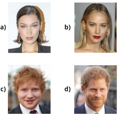
1.1 Images of similar non-kin people, a) to b), and c) to d) - images obtained

from: https://goo.gl/qsgRFU, https://goo.gl/6tnHkN, https://goo.gl/wAhHv8. . 2

1.2 Images of kin people with large age difference- images obtained from: https://goo.gl/6tnHkN, https://goo.gl/wAhHv8, https://goo.gl/AE3E4d, https://goo.gl/fpU3Cj. ... 2

1.3 Approach of previous methods that approximate the old parents face from the child face by reducing aging effects. Desired outputs are showed at last stage... 3

1.4 Approach of previous methods that trained and tested the same method sep-arately for child-young parent and child-old parent pairs with desired outputs. 3 1.5 Approach of of our method that it does not treat differently child-young par-ent and child-old parpar-ents pairs... 3

1.6 The complete proposed method to perform kinship verification. ... 4

2.1 The artificial neuron ... 7

2.2 ReLU - Rectified Linear Unit Activation Function... 8

2.3 Leaky ReLU function: Before activation the information the function is de-fined by:f (x) = ax, and after: f (x) = x ... 8

2.4 ANN - Artificial Neural Network ... 10

2.5 Deep neural network performing face classification - source: [Guo et al. 2016] 11 2.6 Convolutional Neural Network - source: [Guo et al. 2016] ... 12

2.7 Different learning processes between (a) traditional machine learning and (b) transfer learning - source: [Pan and Yang 2010] ... 13

2.8 The Inception module - source: [Szegedy et al. 2015] ... 13

4.1 Gender balance on VGGFace2 dataset (59.3% male), (40.7% female)-source: [Cao et al. 2017]... 20

4.2 The UB Kinface dataset [Shao et al. 2011] ... 21

4.3 Statics of the UB Kinface dataset- source: [Shao et al. 2011] ... 21

4.4 The complete three phase process of the MTCNN - source: [Zhang et al. 2016] 22 4.5 Detailed version of MTCNN architecture - source: [Zhang et al. 2016] ... 22

4.6 Inception-A layer for Inception-ResNet-v1 - source: [Szegedy et al. 2016] ... 25

4.7 Inception-B layer for Inception-ResNet-v1 - source: [Szegedy et al. 2016] ... 25

4.9 FaceNet original model structure [Schroff et al. 2015] ... 26

4.10 Anchors on the training process [Schroff et al. 2015] ... 27

4.11 The linear model that receives the non-negative difference array... 28

5.1 Image samples from the UB Kinface database before and after facial align-ment with MTCNN ... 31

5.2 Cross entropy on training using VGGFace2 ... 33

5.3 Total loss on training using VGGFace2 ... 33

LIST OF TABLES

3.1 Results of other methods on the UB Kinface dataset ... 16

4.1 Tensorflow time to process LFW dataset with MTCNN ... 19

4.2 The FaceNet architecture used on this research ... 27

5.1 Performance of MTCNN on datasets ... 31

5.2 Empirical learning rate for FaceNet training... 32

5.3 Sample of the extracted features from the facial images on the UB Kinface using FaceNet ... 34

5.4 Number of examples used for cross-validation... 35

5.5 Non-negative distance array that is used as input for the linear model ... 35

5.6 Training parameters for the linear model ... 35

5.7 Results of all the leave-one-out cross-validation cycles with original and grayscale images... 36

5.8 Results of all the five-fold cross-validation cycles with the original and grayscale images... 36

5.9 Five-fold cross-validation overall results ... 37

LIST OF SOURCE CODES

4.1 Algorithm that generates grayscale images ... 23

4.2 Function that generates the model ... 28

4.3 Cost function for the linear model... 29

4.4 Optimizer for the linear model ... 29

6.1 Complete linear model code ... 44

6.2 Complete FaceNet model source code with Inception-ResNet-v1 ... 56

6.3 Reduction-A code from FaceNet on Table 4.2 ... 62

6.4 Reduction-B code from FaceNet on Table 4.2 ... 62

6.5 Function that generates the model ... 63

6.6 Cost function for the linear model... 63

6.7 Optimizer for the linear model ... 63

6.8 Script to process dataset images ... 64

6.9 Script to create grayscale images ... 64

6.10 Code that generates grayscale image(convertgrayscale.py)s ... 64

6.11 Script that trains FaceNet ... 65

6.12 Functions that generate the cross-validation dataset for each cycle ... 65

6.13 Inception-A source code for Inception-ResNet-v1 ... 66

6.14 Inception-B source code for Inception-ResNet-v1 ... 67

LIST OF TERMS AND ACRONYMS

ANN Artificial Neural Networks

ConvNets Convolutional Neural Networks

CUDA Compute Unified Device Architecture

DLML Deep Linear Metric Learning

DMML Discriminative Multimetric Learning for Kinship Verification

fcDBN Filtered Contractive Deep Belief Network

LFW Labeled Faces on The Wild

MNRML Multiview Neighborhood Repulsed Metric Learning for Kinship Verification

MTCNN Multi-Task Convolutional Neural Network

P-Net Proposal Network

PDFL Prototype-Based Discriminative Feature Learning for Kinship Verification

R-Net Refine Network

ReLU Rectified Linear Unit

TL Self-Similarity Representation of Weber Faces for Kinship Classification

TL Transfer Learning

TSL Transfer Subspace Learning

Chapter 1

Introduction

Different from the most common facial recognition approaches that mostly try to com-pare similarity, kinship verification is more complicated to solve because people with dis-similar appearances can be kin and people with dis-similar appearances can be non-kin at all [Shao et al. 2011] [Georgopoulos et al. 2018] [Kohli et al. 2017] [Lu et al. 2014]. For in-stance, on Figure 1.1, pairs a-b and c-d are non-kin similar people, this proximity between facial characteristics provides a complex challenge for facial recognition models because it is necessary to identify what features can signal a kin relation to avoid false positives like the ones that it could easily occur between pairs a-b and c-d, for example.

Despite the difficulties to perform kinship verification, humans can identify kinship re-lations at a higher rate than chance, but it is not clear how [Dehghan et al. 2014]. In this research is also added the additional factor of large age variations with the UB Kinface dataset [Shao et al. 2011].

Since the old parent’s face structure is transformed when compared to when they were young [Shao et al. 2011], the age difference increases the distance between the face of child-old parent making it more difficult to identify the kin relation. On Figure 1.2, it is possible to observe two examples of pairs of images (a-b and c-d) that because of the large age differ-ences it would easily prompt a false negative if the model is based solely on the raw facial dis-tance. The age difference present on the UB Kinface dataset makes the problem more chal-lenging [Shao et al. 2011], and it has been treated separately by previous methods available on the literature [Georgopoulos et al. 2018] [Kohli et al. 2017] [Xia 2012] [Yan et al. 2014]

[Yan et al. 2015] [Lu et al. 2014] [Xia et al. 2011] [Shao et al. 2011] [Kohli et al. 2012]. A key factor that inspired this research is the fact that all the other solutions for kinship verification with large age variations using the UB KinFace database, either try to preprocess the face of the old parent to approximate it to the child face as shown in Figure 1.3, or trained the same method twice, one for the young parent pairs, and another for child-old parents pairs like on Figure 1.4.

Figure 1.1: Images of similar non-kin people, a) to b), and c) to d) - images obtained from: https://goo.gl/qsgRFU, https://goo.gl/6tnHkN, https://goo.gl/wAhHv8.

Figure 1.2: Images of kin people with large age difference- images obtained

from: https://goo.gl/6tnHkN, https://goo.gl/wAhHv8, https://goo.gl/AE3E4d,

Figure 1.3: Approach of previous methods that approximate the old parents face from the child face by reducing aging effects. Desired outputs are showed at last stage.

Figure 1.4: Approach of previous methods that trained and tested the same method separately for child-young parent and child-old parent pairs with desired outputs.

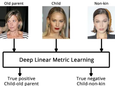
Figure 1.5: Approach of of our method that it does not treat differently child-young parent and child-old parents pairs.

into four stages:

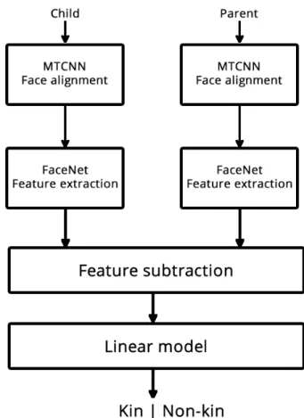
• Face Alignment-MTCNN: Faces are detected and cropped using a Multi-Task Con-volutional Neural Network(MTCNN) [Zhang et al. 2016]. The first phase will provide a picture of the face with 160x160 size as output.

• Feature Extraction-FaceNet: The processed images are then fed onto a

FaceNet [Schroff et al. 2015] [Sandberg 2018] implementation that is going to gen-erate embeddings of 128 dimensions of the face.

• Feature subtraction: The extracted features are subtracted to create an array of 128 dimensions that represents the distance between two faces.

• Linear model: Finally, the distance array of 128 dimensions is fed onto a linear

model that is going to provide a boolean output informing if the two people are kin or not.

Figure 1.6: The complete proposed method to perform kinship verification.

1.1

Applications

• On passports checks because it is necessary to differentiate kin people. Kinship verifi-cation can be used to improve facial recognition models that are sensitive to this type of situation [Georgopoulos et al. 2018].

• Identifying the parents of lost children and orphans to help the work of law enforce-ment agencies [Lu et al. 2014].

• Improving target ads by using the preferences of their kin people to provide a more personalized experience [Georgopoulos et al. 2018].

• To organize family photos detecting kin relations on pictures. • To search for relatives in public datasets [Kohli et al. 2017].

• To allow make-up artists to modify the appearance of two people in a way that they seem blood-related [Georgopoulos et al. 2018].

Our method offers a more practical and simple solution to all of these applications because it discards the need for detecting large age differences.

1.2

Contributions

The contributions of this research are:

• Deep Linear Metric Learning: Until now, all the past solutions have treated kinship verification with large age variations using the UB Kinface dataset as two separate problems, identify a child-young parent kin relation, and identify a kin relation be-tween child-old parent. Our novel DLML method offers a new and more practical solution for kinship verification problem with large age variations, by using an all in one approach that enhances applicability on real-world situations.

• Transfer learning: The results confirmed that the features extracted by our FaceNet model trained with VGGFace2 to perform facial recognition can be re-purposed to perform kinship verification with robustness towards large age variations present on the UB Kinface dataset by applying our linear metric learning approach.

• Results: The results provided by this research showed that the proposed DLML

framework can identify kinship relations despite large age differences and with better performance than multiple other methods.

1.3

Final considerations

On this chapter, the kinship verification with large age variation problem tackled by this research was presented and explained why it is a difficult problem, the components of the

proposed DLML method were explained in a high level. A few applications and the main objectives of the research were presented. The contributions of the research are also cited at the end of the chapter.

It is important to highlight that this research does not have the purpose of discussing/ex-ploring how the kinship relation is detected, only to perform the task. The reason for that is because as stated by [Dehghan et al. 2014], it is not clear how humans can identify kinship relations, because of that, trying to understand how these process works are usually treated as a different type of research. Exploring why the kinship relation exists is an interesting next step for this research, but it is something that on this moment has not yet explored.

Chapter 2

Background

This chapter will present in high level the main resources used on this research.

2.1

The Artificial Neuron

All of our architectures are based on the first artificial neuron model was presented at the decade of 1940, [McCulloch and Pitts 1943], even today this is one of the most used models on artificial intelligence [Goodfellow et al. 2016]. It is inspired by the brain and tries to mimic how human neurons are activated [Rosenblatt 1958]. It can also be called the neuron element [Widrow and Hoff 1960].

Figure 2.1: The artificial neuron

y =

j

X

i=1

wi × xi + w0 (2.1)

As shown at the Equation 2.1 the artificial neuron receives multiple inputs(x1, x2...xn),

each input is multiplied by a correspondent weight(w1, w2...wn), the results are summed up;

a bias(w0) is added to improve the freedom of the model; the outcome of this sum (y) act as

an input to an activation function that will decide if the artificial neuron should be activated or not [Rosenblatt 1958].

2.1.1

Rectified Linear Unit

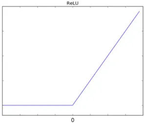
Our FaceNet and MTCNN models use one of the most successful activation functions, the Rectified Linear Unit (ReLU) [Goodfellow et al. 2016]. This function is heavily inspired by how neurons work. As presented on the Equation 2.2, the output of the artificial neu-ron is going to be the maximum value between the sum of inputs and weights (y) and

0 [Goodfellow et al. 2016]. At the Figure 2.2, it is possible to observe that the (w0) bias

is going to set the point of activation of the output, where the output starts to increase ac-cordingly to the input stimulus.

Figure 2.2: ReLU - Rectified Linear Unit Activation Function

Out = max(0, y) (2.2)

2.1.2

Leaky Rectified Linear Unit

−4 −2 2 4 −2 2 4 f(x)=x f(x)=ax x y

Figure 2.3: Leaky ReLU function: Before activation the information the function is defined by:f (x) = ax, and after: f (x) = x

Our linear metric learning model activation function is a variation of the ReLU, the Leaky Rectified Linear Unit (Leaky ReLU) [Xu et al. 2015] is used on the last stage of the model on Figure 1.6, and it is very similar to the ReLU activation function, the only difference is that before the activation the output is defined by a function instead of zero as shown in Figure 2.3. By using a different function before activation loss of information is avoided while the output is not active.

2.1.3

Training

One of the main tasks on the artificial neuron model is to find the best value for the weights that will ensure the right output; this process is called training. On training, the artificial neuron receives inputs that have the desired outputs informed. Each time that the output is wrong, the error is calculated by a given function, and the weights are ad-justed [Goodfellow et al. 2016] [Rosenblatt 1958] [Widrow and Hoff 1960]. This strategy of training is called supervised learning, and after finished, the artificial neuron can operate without having the desired output informed [Goodfellow et al. 2016].

2.1.4

Loss

Loss functions used on training to measure the performance of the prediciton, saying how far the answer is from the desired [Goodfellow et al. 2016]. The values provided by this function will be used on an otimization function in order to try to find the minimum value of the loss function by adjusting the weights. The most common optimization method function for multi-layer ANN’s is called backpropagation.

2.2

Artificial Neural Networks-(ANN)

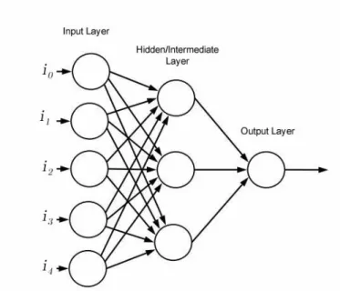
The artificial neuron is a feed-forward model that works as a linear classifier, and because of that, it can only learn simple tasks. It can find out how to mimic an AND function, but it can not learn how to classify one image. To overcome that problem researchers connected multiple layers of artificial neurons(Figure 2.4. That way it is possible to solve complicated problems like image classification [Goodfellow et al. 2016]. When working with images, the inputs(i0, i1, i2, i3, i4) would usually refer to a value between 0 and 255 if the data is black

and white, or a vector of three values between 0 and 255 if the image has color information. With the addition of more layers, the training process is more complicated. Identify what contribution one intermediate/hidden layer has to the error on the output becomes

a challenge. It is necessary to understand what is the role of that layer in the whole

process. The most efficient way to do that task is with a technic called backpropaga-tion [LeCun et al. 1989] [Goodfellow et al. 2016]. Since the outcome of one layer is a

func-Figure 2.4: ANN - Artificial Neural Network

tion of the input of the previous layer, it is conceivable to use a cost function that represents the error and using the derivatives of this function to discover how much each layer con-tributes to the error of the output. After this information is acquired, it is possible to adjust the weights of each layer to improve the result. When working with images, the ANN learns how to extract features of the data on this process [LeCun et al. 2010].

2.3

Backpropagation

As the name suggests, the backpropagation algorithm is a technic to propagate errors back. The method treats each layer of the network as an independent function, and by as-suming that, it is possible to use the chain rule of derivatives in order to understand how each layer is responsible for the error on the last layer [Goodfellow et al. 2016]. One of the most common methods for backpropagation is called gradient descent, this method tries to find the minimum of the loss function. There are also multiple variations of this method, and on this paper the standard backpropagation and the Adam [Kingma and Ba 2015] version are used.

2.4

Deep Learning

The first studies on artificial intelligence solved problems describing a list of formal mathematical rules. That is also known as the classical approach to artificial intelligence. That is exceptional for situations that it is possible to model your problem in mathematical rules, but not useful when dealing with problems that require intuitive knowledge such as face recognition and other computer vision tasks [Goodfellow et al. 2016].

Deep learning is a category of machine learning that uses artificial neural networks

with many layers of artificial neurons, thus the name deep learning. Because of their

depth, these models can solve problems that require intuitive knowledge. With that, it is possible to learn complex concepts without the necessity of model them into mathe-matical rules. Intermediate layers can be trained efficiently using backpropagation algo-rithms [LeCun et al. 2010]. Deep learning models can also be called the modern approach to artificial intelligence [Goodfellow et al. 2016].

Figure 2.5: Deep neural network performing face classification - source: [Guo et al. 2016] Figure 2.5 illustrates a trained deep neural network performing face recognition, where the face of the person of the class P0 is submitted to the system. The system will process the data using three hidden layers, and one output layer, to then give a positive result for the P0 output and a negative result for the remaining classes(P1, P2, P3).

With the recent advances in deep learning, computers were able to provide results that are greater than a person in computer vision tasks such as face recognition and image classi-fication [LeCun et al. 2010].

2.5

Convolutional Neural Networks-(ConvNets)

Convolutional neural networks are one of the most successful artificial neural net-work architectures for feature extraction. These netnet-works are inspired by the neocogni-tron [LeCun et al. 2010] [Goodfellow et al. 2016], a model based on the human visual cor-tex [Fukushima 1980].

Since proposed [LeCun et al. 1989], ConvNets have won major computer vision com-petitions. The state-of-the-art classification algorithm with the best result on the ImageNet Large-Scale Visual Recognition Challenge it is based on a convolutional architecture and has

reached an error of 3.6% [Goodfellow et al. 2016]. The winner architecture of the ImageNet 2014, the inception [Szegedy et al. 2016], is used on this research.

One of the main advantages of ConvNets is the share of weights. After defining

the size of the feature extraction region(Figure 2.6), the same weights will be used to

extract the features of the input. The weight sharing improves the performance,

be-cause the training process becomes more straightforward, and the portion of memory used to store the weights are significantly smaller than the portion used by other archi-tectures [LeCun et al. 1989] [LeCun et al. 2010] [Goodfellow et al. 2016]. Usually, after one or multiple convolutional layers, a pooling layer is used to reduce the dimension-ality of the data minimizing information loss for the next layer as presented on Fig-ure 2.6 [Goodfellow et al. 2016].

Figure 2.6: Convolutional Neural Network - source: [Guo et al. 2016]

2.6

Transfer Learning

Knowledge transfer is something that humans use to learn new complex concepts quickly; They can use knowledge acquired from other experiences to help them under-stand new representations and features of the world [Gutstein et al. 2008](Figure 2.7. Con-vNets can also use the knowledge from one task to learn other tasks faster like humans do [Ranjan et al. 2016]. The most common way to do that with machine learning algorithms, including deep learning models, is to use the weights of an ANN or other characteristics of the model. These trained weights have the abstract representation of the input data to perform the feature extraction from the data.

When working with an ANN to utilize the knowledge acquired on previous tasks, it is possible to train the last layer, what will define if the knowledge can be used for the task at hand, is how much training is necessary to achieve good results. With image related tasks, researches have shown that the cost of retraining a model is small [Ranjan et al. 2016].

Figure 2.7: Different learning processes between (a) traditional machine learning and (b) transfer learning - source: [Pan and Yang 2010]

2.7

Inception Module

The first version of the inception architecture that is used on the original FaceNet is built with the inception module: a mix of layers that run several parallel convolutional layers and concatenate their outputs as presented on Figure 2.8.

The main idea of the inception module is to discover how the best local sparse structure in a convolutional network can be approximated and covered by readily available dense components [Szegedy et al. 2015]. The main benefit of this strategy is the increase of units at each stage without unconstrained computational complexity increase [Szegedy et al. 2015].

2.8

Final considerations

On this chapter the main necessary resources to understand this research were presented, informing the reader about the main necessary aspects to understand this research. These re-sources are artificial neuron, ReLU activation function, Leaky ReLU activation function, the training process for artificial neurons, ANN’s, Deep Learning, ConvNets, Transfer Learning, Inception Module, and Inception-ResNet-v1 modules.

Chapter 3

Related Works

Making kin annotations is more complicated than making annotations of identity

be-cause it is necessary to work with pairs. Inherently, it is more challenging to collect

and annotate the data of the UB Kinface than the data of VGGFace2 that it is mainly

used to detect identity. This complexity led to a scarcity in large kin-related datasets

when compared to traditional datasets such as Labeled Faces on the Wild (LFW) and VG-GFace2 [Georgopoulos et al. 2018].

There is a consensus that the UB Kinface dataset is the kinship dataset with the largest age variations [Georgopoulos et al. 2018]; however, the original paper [Shao et al. 2011] does not provide the values of the age differences among pairs.

All the past solutions that used UB Kinface have focused mainly on achieving good results on the dataset, treating the child-young parent and child-old parent pairs as different problems [Georgopoulos et al. 2018](Figure 1.3 and 1.4. The methods found in the literature are difficult to apply in a real-world environment because they need to detect if there is a big age difference between the two faces to decide what approach should be used.

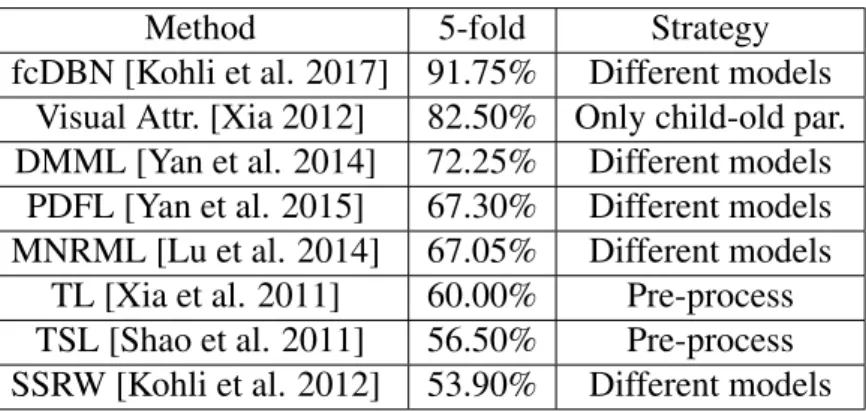
Table 3.1 presents some of the most relevant methods evaluated on the UB-kinface dataset [Georgopoulos et al. 2018]. In Table 3.1, the different models strategy refers to the approach showed on Figure 1.4, and pre-process refers to the approach presented on Fig-ure 1.3, the 5-fold and leave-one-out columns on Table 3.1 are the average accuracy of these methods child-young parents and child-old parents, unlike our method these evaluations are performed separately.

Most of the attempts to solve kinship verification have used shallow machine

learning methods like [Chergui et al. 2018], [Dehghan et al. 2014], [Yan et al. 2014],

[Yan et al. 2015], [Xia et al. 2011], [Shao et al. 2011], [Kohli et al. 2012], [Xia 2012], [Lu et al. 2014]. The only deep learning method evaluated on the UB Kinface dataset used about 600,000 images for train on feature extraction [Kohli et al. 2017], more than five times less than our method that used more than three million images from VGGFace2 as shown on Table 5.1).

Table 3.1: Results of other methods on the UB Kinface dataset

Method 5-fold Strategy

fcDBN [Kohli et al. 2017] 91.75% Different models

Visual Attr. [Xia 2012] 82.50% Only child-old par.

DMML [Yan et al. 2014] 72.25% Different models

PDFL [Yan et al. 2015] 67.30% Different models

MNRML [Lu et al. 2014] 67.05% Different models

TL [Xia et al. 2011] 60.00% Pre-process

TSL [Shao et al. 2011] 56.50% Pre-process

SSRW [Kohli et al. 2012] 53.90% Different models

One of the few deep learning methods available on literature that performed kinship verification on the UB Kinface dataset is called Filtered Contractive Deep Belief Network (fcDBN) [Kohli et al. 2017]. fcDBN is also , to the best of our knowledge, the state of the art method for most of the publicly available datasets, this method used for the first time external datasets to teach the model how to extract facial features to perform kinship verification [Georgopoulos et al. 2018].

In the first stage of fcDBN, the features of each facial region are learned from outside training data. These are learned through the filtered contractive DBN (fcDBN) approach. The learned representations are combined in a compact representation of the face in the second stage. Finally, a multi-layer neural network is trained using these learned feature representations for supervised classification of kin and non-kin [Kohli et al. 2017].

fcDBN was tested on the UB Kinface dataset using five-fold cross-validation and achieved 92.00% of accuracy on child-young parents pairs and 91.50% accuracy on child-old parents pairs [Kohli et al. 2017], 91.75% on average.

The research responsible for publishing the UB Kinface dataset [Shao et al. 2011] used a method called Transfer Subspace Learning(TSL) that uses local Gabor filters to extract features. These features are used to determine if parent and children have similar eyes, noses or mouths. With the extracted key points, six ratios of common regions distances are obtained, e.g., eye-to-eye versus eye-nose distance. The TSL method performs context-aware tests reducing the divergence between child-old parent by using the child-young parent as an intermediate set.

The research presented in [Shao et al. 2011] extracted the features using Gabor filters on each local region. These features are used to determine if parent and children have similar eyes, noses or mouths. With the extracted key points, six ratios of common regions distances are extracted e.g: eye-to-eye versus eye-nose distance. Following a principle that says that these distances are inherited mainly from parents. Structural information is also extracted and following a principle that says that old parent’s structural face is transformed from the one when they were young, because of that a transfer subspace learning method was applied to mitigate the degrading factor. To fully utilize all features, a new strategy called

Cumu-lative Match Characteristic (CMC) is used: features are added in several rounds according to the one that can maximize the difference of recognition performance of child-old parents. After extracting and select the features that will be used for classification a metric learning approach is used, this process will try to use the selected features to choose what features should determine if the two people are kin or not. On their research, they also presented two human baselines for kinship verification that are 53.17% and 56.00%. With 5-fold cross-validation, with 40 positive pairs and 40 negative pairs being left to test the accuracy result 56.5%. With leave-one-out protocol, the achieved accuracy was 69.67% [Shao et al. 2011]. The human baseline shows that the problem tackled by this research is a difficult one.

Another example of research on kinship verification is [Lu et al. 2014]; this paper pro-posed a novel model called Neighborhood Resulsed Metric Learning(NRML). In this case, the relations were separated into four different types: father-son S), father-daughter (F-D), mother- son (M-S), and mother-daughter (M-D) kinship relations. The strategy used by this method tries to repulse interclass samples (without kinship relation) with the higher sim-ilarity that lie in a neighbourhood and approximate the intraclass samples, using the more discriminative information for solve the problem. They also used multiple feature descriptors to try to improve the performance of the method, in this case, it was called Neighborhood Resulsed Metric Learning(MNRML)

Our method differs from fcDBN on the architectures used (MTCNN and FaceNet), on the dataset used to train the network how to extract facial features (VGGFace2). However, the main difference between our DLML and all the previous methods including fcDBN is the fact that our method can detect kin relations on the UB Kinface dataset without treating any age difference, offering enhanced applicability.

Metric learning is used because is one of the most sucessfull methods to solve the kinship verification problem, since it does not need as many data as deep learning methods, and it can separate what features are relevant to detect a kin relation [Georgopoulos et al. 2018].

Furthermore, in our case, to show how expressive the extracted features of our method are to perform kinship verification on the UB Kinface, our last stage is a simple linear artificial neural network.

3.1

Final considerations

In this chapter, the method from the original UB Kinface dataset is

sented [Shao et al. 2011], other methods evaluated on the UB Kinface dataset are also pre-sented and compared to the method proposed in this research. Another important topic ap-proached on this chapter is the state of the art method on the UB Kinface dataset and how this method differs from the proposed DLML method.

Chapter 4

Method: Deep Linear Metric

Learning-(DLML)

Previous methods [Kohli et al. 2017], [Xia 2012], [Yan et al. 2014], [Yan et al. 2015], [Lu et al. 2014], [Xia et al. 2011], [Shao et al. 2011], [Kohli et al. 2012], have trained and evaluated their solutions on child-young parents pairs and child-old parents pairs separately. In this research the contrary is done using the proposed DLML method, making the cross-validation with the whole dataset. This approach is inspired by the fact that ConvNets are bioinspired by the human brain [LeCun et al. 2010] that is the responsible for identify kin-ship relations, thus they can execute intuitive tasks like kinkin-ship verification without the need to be informed what is the age difference of two people.

It is also important to highlight that the phases of the proposed method are not connected, each phase generates an output, that is later used as the input of the next phase. This decision was made in order to try to maximize flexibility during research.

4.1

Hardware and Environment

All the experiments were performed on a laptop with the following configuration: • Processor: Intel(R) Core(TM) i7-4720HQ CPU @ 2.60GHz

• Memory: 16Gb of memory • GPU: GTX970M

All the code developed and from third-parties was developed using Python with environment parameters to allow to run commands via shell script.

The Tensorflow version used was compiled to use multiple sets of instructions that are specific to the GPU, and it improves the performance of the GPU calculations using CUDA.

Measuring by the time necessary to perform facial alignment on the LFW images with the MTCNN architecture, the custom version provided a performance six times better than the general GPU version of Tensorflow, and 21 times better than the CPU version on the same hardware as presented on Table 4.1.

Table 4.1: Tensorflow time to process LFW dataset with MTCNN

Version LFW time (seconds)

CPU 441

GPU 126

GPU for GTX-970M 21

TensorFlow is an open source software library for machine learning that uses data-flow graphics. Nodes represent math operations and the graph edges represent the multidimen-sional data arrays (tensors) that flow among them. This is a flexible architecture that allows deployment of computation to one or more CPUs or GPUs in desptops, servers, or mobile devices without the need of rewriting code. TensorFlow also includes TensorBoard, a data visualization toolkit that is used to generated graphs on this research [Community 2018].

Tensorflow 12.0 was compiled specifically for the GPU GTX-970M using CUDA 10, Python 3.7 and GCC-7.

4.2

Datasets

In this section, the datasets used in the research are explored and some of the necessary operations. All data used will be formed by unconstrained images (on the wild).

4.2.1

Training Datasets for Deep Learning

The images of all the datasets do not have a standard size, to convert and align the face of all images to the necessary 160x160px size to use on the FaceNet implementation used on this research [Sandberg 2018], the MTCNN implementation provided by [Sandberg 2018] is used. This model uses the weights of the original MTCNN [Zhang et al. 2016] on a Ten-sorFlow implementation.

4.2.2

VGGFace2

The VGGFace2 is a large-scale face dataset with large age variations, composed of 3.31 million images of 9131 subjects. It has an average of 362.6 images for each

sub-ject [Cao et al. 2017]. Only the training portion of VGGFace2 that has 8631 classes

and approximately 3.14 million images was used to train the FaceNet implementa-tion [Sandberg 2018]. On Table 5.1 it is displayed how many images compose the training

portion of the VGGFace2 dataset. The features of VGGFace2 are what initially inspired our use of young and old parents images without any special treatment to large age differences. It is assumed that the final model would be robust to large age variations because the VG-GFace2 has a high variation on this aspect. 59.3% of the images of VGGFace are from male subjects as presented on Figure 4.1.

Figure 4.1: Gender balance on VGGFace2 dataset (59.3% male), (40.7%

female)-source: [Cao et al. 2017]

Because the data limitation of kinship datasets and the necessity of data for deep learn-ing methods, it is necessary to use a dataset with a different main purpose than the one of this research, VGGFace2 is used to train and validate FaceNet to extract facial features. FaceNet and VGGFace2 will allow us to leverage the superiority of deep learning models stated by [Georgopoulos et al. 2018] on the kinship verification task.

4.2.3

Labeled Faces on the Wild-LFW

Labeled Faces on The Wild(LFW) was also used additionally as a test dataset for FaceNet on training. LFW has 1680 classes with two or more distinct photos [Huang et al. 2017]; these classes are used to test FaceNet performance on intervals of five epochs of training. Tests are made with this dataset because it is one of the main benchmarks for facial recog-nition tasks [Learned-Miller et al. 2016]. The results obtained on this tests are not used to adjust the weights of the network, only to assess the performance of the trained model with-out bias.

4.2.4

The UB Kinface dataset

UB KinFace dataset is used to perform cross-validation for kinship verification. The dataset is made of 200 group of images composed by old parents, young parents, and chil-dren(total of 600 images). Most of the pictures of young parents are in grayscale because

of the technology available at the time of the photos; there are also other examples of iso-lated grayscale images. In Figure 4.2 examples of pictures from the UB Kinface dataset are exhibited.

Figure 4.2: The UB Kinface dataset [Shao et al. 2011]

The types of kinship relations are not evaluated separately because nearly 80% of the relations are father-son relations as presented on the statics of the dataset at Figure 4.3.

4.3

Multi-Task

Cascaded

Convolutional

Network

(MTCNN)

Figure 4.4: The complete three phase process of the MTCNN - source: [Zhang et al. 2016]

Figure 4.5: Detailed version of MTCNN architecture - source: [Zhang et al. 2016] An MTCNN implementation [Sandberg 2018] is used to perform facial alignment be-cause it provides good performance on hard examples like various poses, illuminations, and occlusions [Zhang et al. 2016]. The MTCNN architecture first resizes the image to different scales to build an image pyramid which will be the input of a three-phase cascade frame-work [Zhang et al. 2016]. The complete frameframe-work can be seen on Figure 4.4 and a detailed version of the MTCNN architecture can be seen on Figure 4.5. The MTCNN facial alignment process is described as follow.

• Proposal Network (P-Net) On the first stage, a fully convolutional neural network find the candidate facial windows and the bounding box regression vectors. These candi-dates are found estimating the borders of the face. After that, a non-maximum sup-pression (NMS) is applied to merge highly overlapped candidates [Zhang et al. 2016]. • Refine Network (R-Net) On the second stage all candidates are processed by another network which discards a significant number of false candidates, executes calibration with bounding box regression, and performs NMS [Zhang et al. 2016].

• Identify Facial Landmark It is similar to the second network, but in this case, the goal is to identify face regions with more supervision, providing five facial landmarks as output [Zhang et al. 2016]

The goal of the research is not performing facial alignment, so, a pre-trained model [Sandberg 2018] that uses the weights provided by the authors of the MTCNN pa-per [Zhang et al. 2016] is used.

The post-MTCNN images will be a stretched version of the face with the size 160x160. The reason to use the stretched face is is that the necessary features for FaceNet are kept after transformation [Schroff et al. 2015], and this allows FaceNet to have the standard input size of 160x160.The The "Original color images" are composed by these images.

These aligned face images of the UB Kinface dataset will also be used to create a new dataset that consists of all the images converted to grayscale(grayscale images. This dataset has the purpose of analyzing the impacts of different channel patterns on the results.

4.4

Converting UB Kinface to grayscale

During tests with the original images from UB Kinface, the results showed that the vari-ance on color channel patterns present on the UB Kinface dataset (colorful and grayscale images) increased the distance between faces and decreased the performance of the linear model. To overcome this increase in distance because of color patterns a grayscale version of the UB Kinface dataset was created.

To create the grayscale version of images that are used for experiments, the algorith presented on List 6.10 is executed.

List 4.1: Algorithm that generates grayscale images

1 f u n c t i o n c r e a t e _ a n d _ s a v e _ g r a y s c a l e _ i m a g e s ( s o u r c e _ i m a g e _ p a t h , o u t p u t _ i m a g e _ p a t h ) { 2 img = l o a d ( s o u r c e _ i m a g e _ p a t h ) 3 i m g _ g r a y = t o _ g r a y s c a l e ( img ) 4 s a v e _ i m a g e ( o u t p u t _ i m a g e _ p a t h ) 5 }

6 7 f u n c t i o n p r o c e s s _ d a t a s e t ( a r g u m e n t s ) { 8 f o l d e r _ p a t h _ l i s t = l o a d _ a l l _ f o l d e r s ( a r g s . r o o t _ d i r _ d a t a s e t ) 9 o u t p u t _ p a t h = a r g u m e n t s . o u t p u t _ d i r _ d a t a s e t 10 f o r ( f o l d e r _ p a t h i n f o l d e r _ p a t h _ l i s t ) { 11 i m a g e _ p a t h _ l i s t = l o a d _ a l l _ f i l e s ( f o l d e r _ p a t h ) 12 f o l d e r _ o u t p u t _ p a t h = o u t p u t _ p a t h + f o l d e r _ p a t h 13 f o r ( i m a g e _ p a t h i n i m a g e _ p a t h _ l i s t ) { 14 s o u r c e _ i m a g e _ p a t h = f o l d e r _ p a t h + i m a g e _ p a t h 15 o u t p u t _ i m a g e _ p a t h = f o l d e r _ o u t p u t _ p a t h + i m a g e _ p a t h 16 c r e a t e _ a n d _ s a v e _ g r a y s c a l e _ i m a g e s ( s o u r c e _ i m a g e _ p a t h , o u t p u t _ i m a g e _ p a t h ) 17 } 18 } 19 }

4.5

FaceNet

The FaceNet architecture used in this research(Table 4.2) has shown one of the best performances on some of the most relevant facial recognition benchmarks like LFW and Youtube Faces Database [Schroff et al. 2015]. Another key factor that inspired the use of FaceNet is the fact that the network generates an array of facial embeddings, assuming the principle that this array can be applied to other purposes, in this research it was used to perform kinship verification.

4.5.1

Inception-ResNet-v1 modules

On the FaceNet implementation used on this research, the Inception-ResNet-v1 is used, this version reduces the computational cost and offers better performance. This Inception version also offers better accuracy and better convergence on training [Szegedy et al. 2016]. The main difference between the classical Inception and the ResNet version is the use of residual connections, that consists in using the output of the previous layer as a direct input to the next layer, with convolutions being performed on paralel [Szegedy et al. 2016]. Residual connections can be observed on Figure 4.6, Figure 4.7, and Figure 4.8.

The Inception-ResNet-v1 is composed of 3 types of inception modules(layers). The first one is the Inception-A that is presented on Figure 4.6, it has a grid of 35x35.

The second one is the Inception-B that is presented on Figure 4.7, it has a grid of 17x17. The third one is the Inception-C that is presented on Figure 4.8, it has a grid of 8x8. To extract features on FaceNet, convolutional, pooling, and inception layers are used as shown at Table 4.2. The convolutional and pooling are done on the first stage; the inception

Figure 4.6: Inception-A layer for Inception-ResNet-v1 - source: [Szegedy et al. 2016]

Figure 4.8: Inception-C layer for Inception-ResNet-v1 - source: [Szegedy et al. 2016]

layer is responsible for extracting mid-level features.

The Reduction-A(layer 13) and Reduction-B(layer 23) layers on Table 4.2 are basically elaborated pooling layers.

FaceNet creates an array of 128 dimensions of the face; those dimensions are used on training to create an abstract representation of the face that it is called anchor. The anchor will have a maximum distance of all representations of that face. It is possible to see the FaceNet method in a simple perspective on Figure 4.9.

Figure 4.9: FaceNet original model structure [Schroff et al. 2015]

On training, the original paper [Schroff et al. 2015] used a triplet loss function. The training process increases the distance of negative samples and approximates the positive samples as shown in Figure 4.10 [Schroff et al. 2015].

Triplet loss is computationally more costly than training as a softmax classifier using cross-entropy loss and training as a classifier can still offer good results [Parkhi et al. 2015]. On this research, Facenet was trained as a softmax classifier with cross-entropy loss.

Table 4.2: The FaceNet architecture used on this research

stage layer type

1 to 3 3 x Convolution 4 Max pooling 5 to 7 3 x convolution 8 to 12 5x Inception-A 13 Reduction-A 13 to 22 10x Inception-B 23 Reduction-B 24 to 28 5x Inception-C 29 Average pooling 30 Flattening layer 31 Fully connected

Figure 4.10: Anchors on the training process [Schroff et al. 2015]

of the inception architecture [Schroff et al. 2015]. In this research, the

Inception-Res1Net-v1 architecture is used because it provides better performance and conver-gence [Szegedy et al. 2016]. The FaceNet implementation used is based on the NN3 archi-tecture of the original paper [Schroff et al. 2015]. This network has input size of 160x160.

To perform testing on the LFW dataset on every epoch of training, the

"Pair Matching" protocol with "Unrestricted, with labeled outside data" provided by [Huang and Learned-miller 2014] is used. The 1680 classes with more than two images are used to form pairs of images without overlapping. These pairs will test the distance be-tween the two embeddings created by the network. A class with four images, for instance, will have two pairs of images to evaluate, [0,1] and [2,3]. This distance is calculated using the euclidean distance between the two embeddings(L2 norm) as described on Eq. 4.1, with

pi as one of the embeddings and qias the other.

[htpb]L2 = v u u t 127 X i=0 (pi− qi)2 (4.1)

The test results on LFW during training are not used to adjust the network weights, only to assess the performance of FaceNet.

4.6

Linear metric learning for kinship verification

The last stage tackles the fact that facial features of similar people lie in a close neigh-borhood, but this does not necessarily mean that these two people are kin, and the contrary is also true. Enters the last phase of our method with the metric learning approach that tries to learn what are the right feature differences to detect kin and a non-kin people.

The extracted features of two images are subtracted forming positive difference pairs like [[1,201], [2,402], ...], and negatives such as [[1,225], [2, 561]]. Considering 1 to 200 as children, 201 to 400 as young parents, and 401 to 600 as old parents.

Figure 4.11: The linear model that receives the non-negative difference array

List 4.2: Function that generates the model

1 f u n c t i o n c r e a t e _ n e t w o r k ( i n p u t _ a r r a y , s i z e _ i n p u t = 1 2 8 , n _ c l a s s e s = 2 , k e e p _ p r o b = 0 . 4 ) { 2 l a y e r _ 1 = d e n s e _ l a y e r ( i n p u t _ a r r a y , s i z e _ i n p u t , a c t i v a t i o n = l e a k y _ r e l u ) 3 d r o p o u t _ l a y e r = d r o p o u t ( l a y e r _ 1 , k e e p _ p r o b ) 4 l a y e r _ 2 = d e n s e _ l a y e r ( d r o p o u t _ l a y e r , n _ c l a s s e s , a c t i v a t i o n = l e a k y _ r e l u ) 5 p r e d i c t i o n = s o f t m a x ( l a y e r _ 2 ) 6 r e t u r n p r e d i c t i o n 7 }

The non-negative result of the subtraction is fed into the linear model of Figure 4.11 that it will perform the kinship verification. The same model is also presented at List 6.5. This model has 128 inputs (same size as the embeddings provided by FaceNet). The first layer has the size of 128x1 with bias unities, and it uses the Leaky Rectified Linear Unit(Leaky ReLu) activation function [Xu et al. 2015].

Next, a fully connected layer with only two outputs finalizes the model, also using the Leaky ReLU activation function. Finally, a softmax function is used to perform the boolean

prediction of kin or non-kin.

On training, dropout [Goodfellow et al. 2016] is applied after the first layer, the

cross-entropy loss function showed on Eq. 4.2 and List 6.6 is used being y_i the predicted value

provided by the model, and y_ilas the expected value. The classical standard backpropagation

algorithm with gradient descent [LeCun et al. 1989] performs optimization of the network during training as shown by the function List 6.7 that it creates the optimizer.

−X

i

y_il· log(y_i) (4.2)

List 4.3: Cost function for the linear model

1 f u n c t i o n c r e a t e _ c o s t _ f u n c t i o n ( model , e x p e c t e d _ v a l u e ) { 2 c o s t _ f u n c t i o n = sum ( e x p e c t e d _ v a l u e ∗ l o g ( model ) 3 r e t u r n c o s t _ f u n c t i o n

4 }

List 4.4: Optimizer for the linear model

1 f u n c t i o n c r e a t e _ o p t i m i z e r ( l e a r n i n g _ r a t e , c o s t _ f u n c t i o n ) {

2 o p t i m i z e r = G r a d i e n t D e s c e n t O p t i m i z e r ( l e a r n i n g _ r a t e , c o s t _ f u n c t i o n ) 3 r e t u r n o p t i m i z e r

4 }

4.7

Final considerations

This chapter presents the hardware used and all the datasets used on this re-search(VGGFace2, LFW, and UB Kinface), the number of images on these datasets is ex-plored, some of specific the characteristics of these datasets are presented, and the available statistics of each dataset are exhibited.

On this chapter it is also presented the proposed DLML method is explained in detail, talking about the specifics of each architecture (MTCNN, FaceNet, linear metric learning model). The fact that MTCNN is not trained as part of this research is explained. The training of the FaceNet architecture is explained, and a comparison between the softmax method used by this research and the triplet loss from original paper is made. The linear metric learning model is explained in detail, and the main algorithms are presented.

Chapter 5

Experiments and results

This section will explore the tasks and experiments made in this research, show and discuss the results of these experiments.

5.1

Face Alignment

Even though face alignment is not a part of the main purpose of this research, it is a necessary step to perform feature extraction with FaceNet and kinship verification with the linear model. MTCNN was the architecture choosed because deep ConvNets architectures, to the best of our knowledge, are the state of the art solution to deal with unconstrained images [Goodfellow et al. 2016], MTCNN has also consistently outperformed the state-of-the-art methods across several challenging benchmarks [Zhang et al. 2016]. MTCNN was also used on the original VGGFace2 article [Cao et al. 2017] to perform facial alignment.

Since face alignment is not one of the main tasks of this research, the model used was the one that it is provided with the FaceNet implementation used on this re-search [Sandberg 2018]; this model is implemented using Tensorflow, the original is im-plemented on Matlab [Zhang et al. 2016]. However, the authors from the original paper published the original code and model as open-source, and the implementation used in this research imports the weights of the original model into the new implementation.

Facial alignment is performed using MTCNN for three datasets: VGGFace2(FaceNet training), LFW(FaceNet testing), and UB Kinface (kinship verification cross-validation). To process the images of the datasets MTCNN is executed for each dataset.

That is a –margin option on the implemented code, the margin would add additional space between the border and the detected face of the image. The margin option was kept as 0 because about half of the images on UB Kinface have face area smaller than 160x160px, adding a margin would reduce even further the quality of half of the post-MTCNN facial im-ages, that it already had to be reduced on 311 of 600 cases(51.83%) to stretch to 160x160px.

The post-MTCNN images of all datasets will have 160x160px, that size is necessary to use the images as input on the FaceNet architecture, the images will be a stretched version of the aligned face to fit on this dimension. On Figure 5.1 it is possible to see samples of images from UB Kinface before and after facial alignment. The MTCNN implementation used also provides information about the facial bounding boxes detected on the images; this allows calculating the size of the facial area for each image.

Figure 5.1: Image samples from the UB Kinface database before and after facial alignment with MTCNN

The performance of the MTCNN pre-trained model [Sandberg 2018] on the three datasets is exhibited on Table 5.1, the before column shows how many images were available before facial alignment, the after shows how many were successfully aligned, and the per-formance is calculated by comparing how many of the images were processed successfully.

Table 5.1: Performance of MTCNN on datasets

Before After Performance

VGGFace2 3,141,890 3,138,862 99.90%

LFW 13,233 13,233 100%

UB Kinface 600 600 100%

From a total of 3,155,723 images 3,152,695(99.90%) images were successfully aligned as presented on Table 5.1. These results showed that the MTCNN architecture performed well on the unconstrained(on the wild) image data used on this research; the post-MTCNN images will allow the next necessary steps(feature extraction and kinship verification) to take place.

5.2

Feature extraction with FaceNet

This section will discuss the training, testing, validation, and use of FaceNet on this research to extract features from facial images.

Because of the specific size and border used on our research to avoid decreasing in image quality, and the large age variation present on our data for kinship verification (UB Kinface) we had to train our own model to perform feature extraction with VGGFace2, this model is tested on LFW and it is responsible for creating the 128x600 dimensions array of features of the 600 images of the UB Kinface dataset.

5.2.1

Training

FaceNet is trained with a total of 500 epochs, each epoch has 1000 batches and each batch has 40 images.

To improve performance and avoid overfitting the fixed image standardiza-tion(normalization) [Goodfellow et al. 2016] technic and dropout [Goodfellow et al. 2016] are used. Table 5.2 displays the empirical learning rate used for training with the Adam optimizer [Kingma and Ba 2015].

Table 5.2: Empirical learning rate for FaceNet training

Epoch Learning Rate

0-99 0.1

100-299 0.05

300-399 0.005

400-499 0.0005

5.2.2

Validation

A portion of 0.01% of the VGGFace2 is used for validation on training to calculate the loss and adjust the weights using the Adam optimizer [Kingma and Ba 2015]. The total sum of the cross-entropy loss can be seen in Figure 5.3. The cross entropy loss value of every batch can be observed in Figure 5.2.

5.2.3

Testing

The accuracy of testing on LFW exhibited at Figure 5.4 is calculated every five epochs using the euclidean distance. After completing training, tests are run again on LFW using the euclidean distance; the accuracy was 98.83%.

After trained with a softmax classifier at the last layer [Parkhi et al. 2015], FaceNet was able to successfully detect and export the features for the 600 images of the UB Kinface

Figure 5.2: Cross entropy on training using VGGFace2

Figure 5.3: Total loss on training using VGGFace2

Table 5.3: Sample of the extracted features from the facial images on the UB Kinface using FaceNet

Feature 0 Feature 1 ... Feature 127

Image 0 (Child) -0.027277473360300064 -0.08217132836580276 ... 0.06560494750738144 ... ... ... ... ... Image 200 (Young-parent) 0.10031850636005402 -0.0060198549181222916 ... 0.08803482353687286 ... ... ... ... ... Image 230 (Young-parent) -0.0584646500647068 -0.12933146953582764 ... 0.08840493857860565 ... ... ... ... ... Image 400 (Old-parent) 0.15667474269866943 -0.13348889350891113 ... -0.04572216048836708 ... ... ... ... ... Image 493 (Old-parent) -0.016640465706586838 0.03600674122571945 ... -0.10782409459352493 ... ... ... ... ... Image 600 (Old-parent) -0.060755062848329544 -0.03715011477470398 ... 0.0024316716007888317

dataset. The values will range from -1 to 1 because of normalization, and this values will be used to create the non-negative array that it will serve as input for the linear metric learning model. On Table 5.3 it is possible to see the structure of the extracted features and a sample of the values.

When presented with a grayscale image, FaceNet will basically represent the grayscale image in three color channels, keeping the grayscale aspect of the data. Even though FaceNet was trained and tested with colorful images from the VGGFace2 and LFW datasets respec-tively, the results on the kinship-verification cross-validation showed that FaceNet was able to extract expressive features from grayscale images.

5.3

Cross-validation on the kinship verification linear

met-ric learning model

Because of the size of UB Kinface dataset, it is recommended to use cross-validation methods to perform tests [Georgopoulos et al. 2018], since if tested with only one model, the results could easily be biased because of the small amount of data. Because of the cross-validation approach, there are also multiple models instead of just one.

The dataset used for cross-validation is composed of 800 image features pairs as de-scribed on Table 5.4, the dataset is mounted in a balanced way that follows the structure: [true child-old parent, false child-old parent, false child-young parent, true child-young par-ent, true child-old parpar-ent, ...].

The negative child-young parent’s pairs are composed of non-kin pairs between child and other young parent individuals, the negative child-old parent’s pairs are made of non-kin pairs of child and old parent individuals. This pattern will repeat throughout the 800 available samples to assure that the tests are well balanced between the four types of examples, that way on each cross-validation cycle, there will always be a balanced number of type examples on training and testing.

Table 5.4: Number of examples used for cross-validation

Type of Relations Positive Negative

Child-young parent 200 200

Child-old parent 200 200

Table 5.5: Non-negative distance array that is used as input for the linear model

Pair Type Distance 0 Distance 1 ... Distance 127 0-400 True Child-Old Parent 0,18395221605897 0,066887825727463 ... 0,111327107995749 0-493 False Child-Old Parent 0,010637007653713 0,102607809007168 ... 0,173429042100906 0-230 False Child-Old Parent 0,031187176704407 0,062730401754379 ... 0,022799991071224 0-200 True Child-Young Parent 0,127595979720354 0,060581212863326 ... 0,022429876029492 1-401 True Child-Old Parent 0,102011129260063 0,246223147958517 ... 0,049301842227578

... ... ... ... ...

A sample of the non-negative array that measures the distance between image features of the UB Kinface is presented on Table 5.5; The array will repeat the presented structure on every 4 items until it reaches the combination of number 800, it is also possible to observe that the child image is used as anchor to generate the 4 types of relations for each iteration. This structure is what guarantees that the data for cross-validation-cycles have a balanced number of types of examples on the training and testing parts.

The cross-validation data is created by iterating through the array of 800 distances em-beddings in an orderly manner. For the leave-one-out protocol, for example, 80 images are used for test per cycle: cycle 1: 0-79, cycle 2: 80-159, ... ; The rest of the data is always used for training. Because of the balanced aspect of the dataset, the cross-validation cycle will not be biased to a specific type of relation. For the five-fold-cross validation, the same process is executed but with 160 images for test per cycle.

Table 5.6: Training parameters for the linear model

Learning Rate Epochs Batch Size Dropout

0.07 10 10 0.4%

The 800 pairs of images of the UB Kinface are tested with the 5-fold cross-validation protocol and leave-one-out protocol with the original images and grayscale images; these tests will create a total of 15 different models (10 for leave-one-out and 5 for five-fold) for original images and 15 models for the grayscale images. The training parameters used to train the models are showed on Table 5.6.

The results for all the leave-one-out cycles can be seen on Table 5.7, and the results for all the five-fold cycles are presented on Table 5.8.

On Table 5.7, it is possible to observe that the leave-one-out protocol with grayscale images offered the best accuracy on very cycle of tests, it is also possible to see decrease in accuracy, precision and recall with the original images because of heterogeneous color patterns present on the UB Kinface dataset, this characteristic also generated a few outliers

Table 5.7: Results of all the leave-one-out cross-validation cycles with original and grayscale images

Leave-one-out cross-validation results

Original images Grayscale images

Cycle Test pair interval Accuracy Precision Recall Accuracy Precision Recall

0 0-79 0.488 0.491 0.700 0.725 0.688 0.825 1 80-159 0.438 0.368 0.175 0.788 0.795 0.775 2 160-239 0.462 0.467 0.525 0.675 0.646 0.775 3 240-319 0.462 0.468 0.550 0.662 0.638 0.750 4 320-399 0.400 0.278 0.125 0.700 0.674 0.775 5 400-479 0.412 0.360 0.225 0.638 0.593 0.875 6 480-559 0.512 0.516 0.535 0,725 0.705 0.775 7 560-639 0.488 0.490 0.600 0.750 0.685 0.925 8 640-719 0.438 0.429 0.375 0.725 0.680 0.850 9 720-799 0.563 0.568 0.525 0.762 0.698 0.925

Table 5.8: Results of all the five-fold cross-validation cycles with the original and grayscale images

Five-fold cross-validation results

Original images Grayscale images

Cycle Test Pair Interval Accuracy Precision Recall Accuracy Precision Recall

0 0-159 0.412 0.436 0.600 0.681 0.704 0.625

1 160-319 0.419 0.240 0.750 0.688 0.636 0.875

2 320-479 0.400 0.389 0.350 0.681 0.649 0.788

3 480-639 0.431 0.441 0.513 0.625 0.601 0.750

4 640-799 0.419 0.440 0.600 0.694 0.663 0.788

on the original images with precision and recall (0.278 for precision and 0.125 for recall). Most of the cycles had similar results, on the grayscale images, for instance, the maximum accuracy difference between two cycles is 0.15 (15.00%), the maximum precision difference is 0.157 (15.70%), and the maximum recall distance is 0.175 (15.50

The results presented for accuracy with grayscale images at Table 5.7 showed that the proposed method, on every cycle of the cross-validation process, has better accuracy then the human baseline, consistently performing kinship verification on the UB Kinface dataset; The precision values show that the DLML proposed method offers better than 60% performance on 90% of the cycles to detect positive kinship pairs when considering all positive pairs on the data, that means that on most cycles the model is correct on 60% of times. The recall values showed that on every cycle the model identifies above 75% of positive kinship relations.

On Table 5.8 it is possible to observe that on the five-fold cross-validation tests the model performs better with the homogeneous grayscale color dataset created, accuracy and preci-sion are always above 60.00% , that means that on more than 60.00% of time the answer is right, and more than 60% of the positive examples classified the model are correct. Con-sidering the recall, it is also possible to affirm that on 80.00% of cycles the model correctly