Equity valuation of Continental AG

(1)

Católica-Lisbon School of Business and Economics

International Master of Science in Management

Equity Valuation of Continental AG

MSc Dissertation

Student Felix Manfred Fries

Student-Number 152114308

Dissertation written under the supervision of Henrique Bonfim.

Dissertation submitted in partial fulfilment of requirements for the International MSc in Man-agement, at the Universidade Católica Portuguesa, 19.12.2016.

(2)

ii

Abstract

The subsequent master’s thesis comprises a valuation of the equity stake of Continental AG (Conti), a German 1st_{tier automotive supplier which is globally active through its Automotive,}

Tire as well as ContiTech divisions.

Therefore, the current state of the art concerning the field of equity valuation is presented and the most appropriate methods for Conti are chosen. Those are a Discounted Cash Flow (DCF) approach with the Weighted Average Cost of Capital (WACC) and a multiples approach using the Sum of Parts (SOP) of Conti’s single divisions. Subsequently, a profound analysis of the automotive industry as well as an internal analysis of Conti itself is presented.

Afterwards, the main part of the thesis presents the drafted financial model and issues the in-vestor a hold recommendation with a target share price of EUR186 dated on 31st_December

2016. This evaluation also includes a sensitivity analysis considering various scenarios for the business development of Conti and a Value at Risk (VaR) assessment using a Monte Carlo simulation for predicting the maximum possible daily loss respectively gain. Moreover, a com-parison of the author’s valuation and a valuation of Exane BNP Paribas is composed.

(3)

iii

Resumo

A presente tese de mestrado compreende a avaliação da participação da Continental AG (Conti), uma reconhecida fornecedora da indústria automobilística alemã, globalmente ativa através das suas divisões: Automóvel, Pneus e ContiTech.

Por conseguinte, é apresentado o atual estado da arte relativamente à avaliação do capital próprio da Conti, através dos métodos mais adequados: Discounted Cash Flow (DCF) em conjunto com o Weighted Average Cost of Capital (WACC) e uma abordagem aos Múltiplos, utilizando a Sum of Parts (SOP) das divisões individuais da Conti. Subsequentemente, é apresentada uma análise profunda da indústria automobilística, bem como uma análise interna da própria Conti.

Posteriormente, a parte principal da tese apresenta o modelo financeiro elaborado e dirige uma recomendação aos investidores expressa num preço alvo por ação de 186 euros, a 31 de dezembro de 2016. Esta avaliação também inclui uma análise de sensibilidade considerando vários cenários para o desenvolvimento da Conti e uma análise do Value at Risk (VaR) utilizando uma simulação pelo Método de Monte Carlo com o intuito de prever a perda diária máxima respectivamente ganha. Adicionalmente, é feita uma comparação entre a avaliação do autor e uma avaliação da Exane BNP Paribas.

(4)

iv

Acknowledgements

First of all, I want to thank my supervisor Henrique Bonfim and my thesis seminar teacher José Carlos Tudela Martins, who always offered me time, support and the necessary guidance to fulfil the thesis requirements.

Second, I want to thank all of my family members, namely my mother, my father and my sister. They always supported me with their guidance, motivation and encouragement not just through-out the whole master program but also throughthrough-out my whole life.

Last, a big thank you goes to all of my friends, who were always there for me and offered advice for this thesis. More specifically, this includes Robin Schrag as well as Martin Wist.

(5)

v

4.3 Share Performance ... 24 4.4 Shareholder Structure ... 24 5 Valuation ... 25 5.1 Methodology ... 25 5.2 Financial Forecasts ... 26 5.2.1 Sales ... 26 5.2.2 EBITDA Margin ... 29 5.2.3 D&A ... 30 5.2.4 CAPEX ... 31 5.2.5 NWC ... 32 5.2.6 Tax Rate ... 33 5.2.7 FCFF ... 33 5.3 Peer Group ... 35 5.4 Cost of Capital ... 36

5.4.1 Target Capital Structure ... 36

5.4.2 Beta ... 37

5.4.3 Cost of Equity ... 38

5.4.4 Cost of Debt ... 39

5.4.5 WACC and Unlevered Cost of Capital ... 39

5.5 Debt Valuation ... 41

5.6 DCF Valuation ... 42

5.7 Multiples Valuation ... 44

5.8 Scenario Analysis ... 44

5.9 Value at Risk ... 46

6 Valuation Comparison with Exane BNP Paribas ... 48

7 Conclusion ... 50

8 Appendix ... 51

(7)

vii

List of Abbreviations

ADAS Advanced Driver Assistance System

Approx. Approximately

APT Arbitrage Pricing Theory

APV Adjusted Present Value

AR Annual Report

B Book Value of Equity

BC Bankruptcy Costs

CAGR Compound Annual Growth Rate

CAPEX Capital Expenditures

CAPM Capital Asset Pricing Model

CoC Cost of Capital

COGS Cost of Goods Sold

Conti Continental AG

D&A Depreciation, Amortization and

Impair-ment

DAX Deutscher Aktienindex (German

High-Cap Stock Index)

DCF Discounted Cash Flow

DPS Dividends per Share

EBIT Earnings before Interest and Taxes

EBITDA Earnings before Interest, Taxes,

Deprecia-tion, Amortization & Impairment

ECB European Central Bank

EPS Earnings per Share

(8)

viii

EUR Euro (Currency)

EV Enterprise Value

FCFD Free Cash Flow to Debt

FCFE Free Cash Flow to Equity

FCFF Free Cash Flow to the Firm

FED United States Federal Reserve

FY Financial Year

GDP Gross Domestic Product

HMI Human Machine Interface

i.e. Id est (“that is to say”)

ICS Industry Classification System

IMF International Monetary Fund

IR Interim Report

LV Light Vehicle

M Million

M&A Mergers and Acquisitions

MDAX Mid-Cap DAX

MEUR Million Euros

NAFTA North American Free Trade Association

NOPLAT Net Operating Profit Less Adjusted Taxes

OEM Overall Equipment Manufacturer

OPEC Organization of the Petroleum Exporting

Countries

OTC Over the Counter

(9)

ix

PPE Property, Plant and Equipment

PPS Price per Share

Q Quarter

R&D Research & Development

ROCE Return on Capital Employed

ROIC Return on Invested Capital

S&P Standard & Poors (Rating Agency)

Schaeffler Schaeffler AG

SGA Selling, General and Administrative

Ex-penses

SIC Standard Industrial Classification

SOP Sum of Parts

TS Tax Shield

U.S. United States of America

VaR Value at Risk

WACC Weighted Average Cost of Capital

WC Working Capital

(10)

x

List of Tables

Table 1: Equity Multiples (Source: Fernández, 2001) ... 4

Table 2: Asset Multiples (Source: Fernández, 2001) ... 5

Table 3: Growth Referenced Multiples (Source: Fernández, 2001) ... 5

Table 4: Automotive – Sales by Region (Source: Continental AR, 2015) ... 26

Table 5: Automotive – Sales Forecast (Source: Own Calculations) ... 27

Table 6: Tire – Sales by Region (Source: Continental AR, 2015) ... 27

Table 7: Tire – Sales Forecast (Source: Own Calculations) ... 28

Table 8: ContiTech – Sales by Region (Source: Continental AR, 2015) ... 28

Table 9: ContiTech – Sales Forecast (Source: Own Calculations) ... 28

Table 10: Automotive – FCFF Forecast (Source: Own Calculations) ... 33

Table 11: Tire – FCFF Forecast (Source: Own Calculations) ... 34

Table 12: ContiTech – FCFF Forecast (Source: Own Calculations) ... 34

Table 13: Peer Benchmarks by Division (Source: Own Calculations) ... 36

Table 14: Final Peer Groups by Division (Source: Own Calculations) ... 36

Table 15: Target Capital Structure by Division (Source: Own Calculations) ... 37

Table 16: Beta Unlevered and Re-Levered (Source: Own Calculations) ... 38

Table 17: Cost of Equity by Division (Source: Own Calculations) ... 38

Table 18: Cost of Debt – Rating Approach (Source: Own Calculations) ... 39

Table 19: WACC by Division (Source: Own Calculations) ... 40

Table 20: Unlevered Cost of Capital by Division (Source: Own Calculations) ... 40

Table 21: Indebtedness (Source: Continental AR, 2015) ... 41

Table 22: Debt Valuation – Bonds Traded (Source: Thomson Reuters Eikon) ... 41

Table 23: Fair Value of Debt (Source: Own Calculations) ... 42

Table 24: DCF Valuation – D/E at Industry Median (Source: Own Calculations) ... 42

Table 25: DCF Valuation – D/E at Current Ratio (Source: Own Calculations) ... 43

Table 26: DCF Valuation – PPS (Source: Own Calculations) ... 43

Table 27: Multiples Valuation – PPS (Source: Own Calculations) ... 44

Table 28: Sales and EBIT Comparison (Source: Own Calculations) ... 49

(11)

xi

List of Figures

Figure 1: Real GDP Growth Rate (Source: IMF, 2016) ... 17

Figure 2: Inflation Rate (Source: IMF, 2016) ... 17

Figure 3: LV Sales Growth Rate (Source: IHS Automotive, 2016) ... 18

Figure 4: Value Chain – Automotive Industry (Source: Noealt, 2009) ... 19

Figure 5: Continental – Divisions (Source: Continental AR, 2015) ... 21

Figure 6: Share Price Performance (Source: Thomson Reuters Eikon) ... 24

Figure 7: EBITDA Margin by Division (Source: Own Calculations) ... 30

Figure 8: D&A as a (%) of Sales by Division (Source: Own Calculations) ... 31

Figure 9: Capex as a (%) of Sales by Division (Source: Own Calculations) ... 32

Figure 10: NWC as a (%) of Sales by Division (Source: Own Calculations) ... 33

Figure 11: Valuation Overview – PPS (Source: Own Calculations) ... 46

Figure 12: Histogram – Monte Carlo Simulation (Source: Own Calculations) ... 47

(12)

xii

List of Equations

Equation 1: FCFF Computation (Source: Berk & DeMarzo, 2007) ... 6

Equation 2: FCFE Computation (Source: Berk & DeMarzo, 2007) ... 7

Equation 3: Beta Levered – Formula (Source: Damodaran, 1999a) ... 8

Equation 4: Beta Levered – Regression Analysis (Source: Damodaran, 1999a) ... 8

Equation 5: Beta Adjusted (Source: Blume, 1971) ... 9

Equation 6: Beta Unlevered (Source: Fernández, 2003) ... 9

Equation 7: CAPM (Source: Black et al., 1972) ... 10

Equation 8: Fama and French 3-Factor Model (Source: Fama & French, 1992) ... 10

Equation 9: Arbitrage Pricing Theory (Source: Ross, 1976) ... 11

Equation 10: Interest Coverage Ratio (Source: Berk & DeMarzo, 2007) ... 11

Equation 11: After-Tax Cost of Debt (Source: Damodaran, 2002) ... 11

Equation 12: WACC (Source: Fernández, 2010) ... 12

Equation 13: Valuation – FCFF at WACC (Source: Fernández, 2013) ... 12

Equation 14: Terminal Value Computation (Source: Fernández, 2013) ... 13

Equation 15: Valuation – FCFE at Cost of Equity (Source: Koller et al., 2010) ... 13

Equation 16: Valuation – FCFD at Cost of Debt (Source: Koller et al., 2010) ... 14

(13)

1

1 Introduction

The goal of this master’s thesis is to determine the equity value of Continental AG (Conti). Conti is a German DAX-listed company, located in Hannover, and is worldwide active through its Automotive, Tire as well as ContiTech division (Continental AR, 2015).

1.1 Motivation

The motivation for this work stems from the fact that the global automotive industry is in the middle of a rapid change. Autonomous driving, connectivity/digitalization, electrification and shared mobility are just a few buzzwords to highlight the most current trends (Continental AR, 2015; Hirsch, Kakkar, Singh, & Wilk, 2015). Consequently, the question which needs to be answered is how this affects Conti, as it is one of the three largest 1st_{tier suppliers within this}

industry and if it is able to adapt to those trends (Statista, 2016a). Since the corporation is also engaged in various businesses and geographical areas, its diversified structure is another fact which makes it an interesting and complex object for a valuation.

1.2 Research Question and Structure

Because the objective of this master’s thesis is the investigation of Conti’s intrinsic equity value, the research question is formulated as follows:

 What is the value of Continental AG’s equity at 31st_{December 2016?}

This comprises a step-by-step evaluation, done according to the following sub-questions: o What is the state of the art in equity valuation and what are the most

appropri-ate methods to use for valuing Conti?

o What are the current industry trends? How do they affect the company? o How does the company run its business and how is it internally structured?

Does its strategy match the current industry trends?

First, a literature review will be presented to introduce the most up-to-date concepts in the field of equity valuation.

Afterwards, an industry analysis is conducted which focuses onto the automotive industry (Continental AR, 2015).

Before the final valuation, an internal company analysis is composed. In general, this includes Conti’s firm structure, its corporate and financing strategy as well as stock-related information.

(14)

2 The final valuation is subsequently executed according to the Discounted Cash Flow (DCF) as well as the multiples method, using a Sum of Parts (SOP) approach.

The results of the valuation will then be compared to an investment bank report of Exane

BNP Paribas. It will be highlighted if and why the results of the author are deviating from their

values.

(15)

3

2 Literature Review

The following section contains the state of the art concerning equity valuation and presents the most suitable approaches for the valuation of Conti.

2.1 Relative Valuation

In a relative valuation, one tries to value an asset by comparing it to the prices of similar assets on the market. The question to be answered is “how much is the market paying for the asset? (Damodaran, 2006).” Nonetheless, this approach just works if the markets are efficient, i.e. if they are not over- or undervaluing an asset. Therefore, the process of a relative valuation com-prises exactly three steps. The first is to find comparable assets that are priced by the market. In case of this thesis this is done via a peer group analysis for comparable companies of Conti. The second step is to scale the market prices to a common variable, namely to so called multiples. Least, adjustments to the obtained multiples have to be done, if there are extraor-dinary factors (e.g. impairment) which make them deviate from their peers (Damodaran, 2006). It has to be mentioned that many academics hold the opinion that a relative valuation is a useful tool for a comparison after a profound intrinsic valuation had already been conducted and not suitable on a standalone basis (Fernández, 2001).

2.1.1 Peer Group

In a more narrow sense, a peer group is a set of comparable companies operating in the same industry as the company being valued. There are various studies attempting to elaborate ways of identifying the closest peers of a specific enterprise. First, some authors defend using Indus-try Classification Systems (ICS) like the Standard Industrial Classification (SIC), Dow Jones or Yahoo for ascertaining peers. Thereby, the accuracy of the final output is strongly correlated to the accuracy of the ICS. The better the classification system, the better the peer group and the more accurate the final multiples (Eberhart, 2004). Furthermore, because ICS are loosely defined, some academics argue for a further refinement of this approach. They state that com-panies being even active in the same industry can deviate significantly in terms of fundamentals as growth rate, Return on Invested Capital (ROIC) or their capital structure. Consequently, the authors propose to use the ROIC as well as the growth rate as an additional evaluation criteria applied to the ascertained companies from the same industry (Bhojraj & Lee, 2002; Goedhart,

(16)

4 Koller, & Wessels, 2005). A second approach is introduced by Damodaran (2005) who men-tions that companies do not have to operate in the same industry if they are equal concerning fundamentals as beta, Earnings per Share (EPS) or growth rate. This is especially helpful in industries with only few incumbents, making it hard to ascertain a vast sample of comparables, because the wider definition criteria increases the sample size.

2.1.2 Types of Multiples

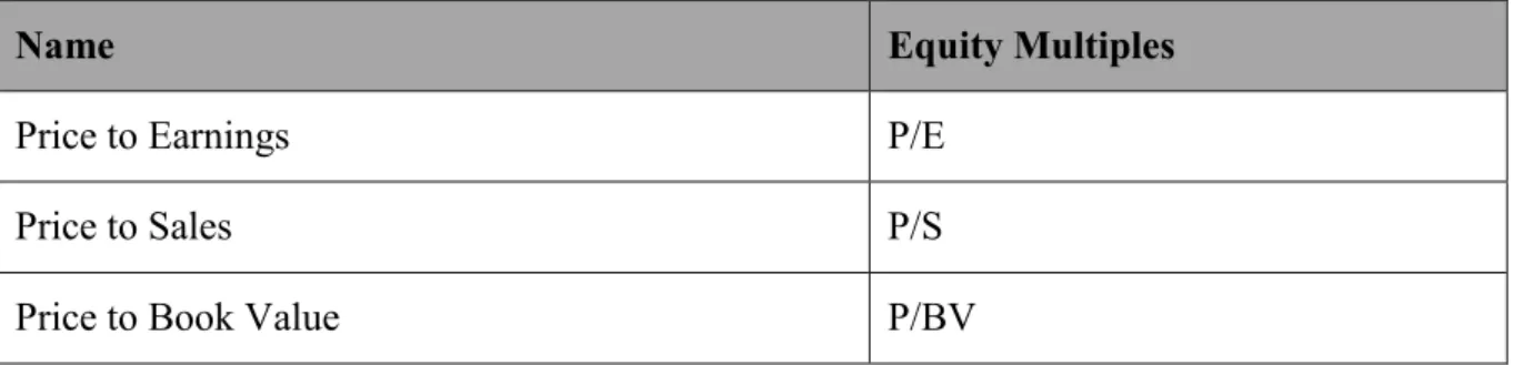
In order to be able to compare the fundamentals of various peers, they are scaled down to a common ratio called multiple (Damodaran, 2005). There are various multiples and opinions on how to categorize them, but in this thesis they are separated into equity (company’s market capitalization) (Table 1), asset (market capitalization + debt) and growth referenced multiples (Fernández, 2001). This is for the sake of clarity.

Table 1: Equity Multiples (Source: Fernández, 2001)

Name Equity Multiples

Price to Earnings P/E

Price to Sales P/S

Price to Book Value P/BV

Multiples based on market capitalization are principally easy to compute and to interpret. Nev-ertheless, the P/E ratio, which is most often used, has the drawback of being affected by the leverage of the respective company. The higher the leverage, the lower the P/E ratio – even though the company’s performance might be the same (Fernández, 2001). In addition, many non-operating items such as write-offs might artificially distort the denominator of the multiple (earnings) (Goedhart et al., 2005; Foushee, Koller, & Mehta, 2012). Furthermore, the future growth rate of the evaluated company has a significant effect on the numerator of the multiple (price) (Goedhart et al., 2005).

Asset multiples use the Enterprise Value (EV) as the numerator for the ratio computation (Fer-nández, 2001) (Table 2).

(17)

5

Table 2: Asset Multiples (Source: Fernández, 2001)

Name Asset Multiples

Enterprise Value to EBITDA EV/EBITDA

Enterprise Value to EBIT EV/EBIT

Enterprise Value to Sales EV/Sales

Foushee et al. (2012) as well as Goedhart et al. (2005) argue for the application of asset instead of equity multiples, because they are not distorted by the above mentioned limitations that affect earnings. Sales multiples are rather considered a bad estimate as it could, based on high sales levels, lead analysts to assign firms high EVs, even though the firms might have low or even no earnings (Damodaran, 2002).

Least, growth referenced multiples are an equity or an asset multiple combined with the growth rate of the company being evaluated (Fernández, 2001) (Table 3).

Table 3: Growth Referenced Multiples (Source: Fernández, 2001)

Name Growth Referenced Multiples

Price to Earnings Growth P/EG

Enterprise Value to Earnings Growth EV/EG

There are various opinions in literature about which multiples to use for the respective industry. Goedhart et al. (2005) as well as Lie & Lie (2002) agree that the manner in which you use the multiple is more significant than the ratio itself. They also concur that it is more accurate to use forward/leading multiples compared to trailing multiples.

It has to be mentioned that, in specific cases, adjustments have to be done to the multiples to account for extraordinary events in the history of the company (Damodaran, 2006).

(18)

6

2.2 Discounted Cash Flow Valuation

The Discounted Cash Flow Methods (DCF) aim at determining a company’s value by discount-ing its estimated future free cash flows at a risk-adjusted discount rate. Conceptually, it can be considered the only correct valuation method (Fernández, 2013).

2.2.1 Free Cash Flows

In general, one can decide between three different free cash flows: Free Cash Flow to the Firm

(FCFF), Free Cash Flow to Equity (FCFE) and Free Cash Flow to Debt (FCFD). Cash

flows express the cash being available to a certain party and can be computed in various ways, starting from Net Income, EBITDA, etc. (Berk & DeMarzo, 2007; Fernández, 2013). For the purpose of this thesis, the starting point for the free cash flow computation is the EBIT. According to Pinto, Henry, Robinson, & Stowe (2007), the FCFF can be described as the cash being available to all capital providers of the company (equity and debt holders), after the pay-ments of all operating expenses (unlevered taxes included), necessary investpay-ments in working capital (WC) as well as fixed assets have been made (Equation 1).

Equation 1: FCFF Computation (Source: Berk & DeMarzo, 2007)

The FCFE is the cash being available for the distribution to the stockholders of the company. To obtain the FCFE, one needs to deduct interest payments after taxes (because it is tax deduct-ible) and principal payments from the FCFF and add new debt issued (Pinto et al., 2007; Fer-nández, 2013) (Equation 2).

-Net Operating Profit Less Adjusted Taxes (NOPLAT) +

-Free Cash Flow to the Firm (FCFF)

Earnings before Interest and Taxes (EBIT) Taxes on EBIT (Unlevered Taxes)

Depreciation and Amortization (D&A) Investments in Net Working Capital (ΔNWC) Capital Expenditures (CAPEX)

(19)

7

Equation 2: FCFE Computation (Source: Berk & DeMarzo, 2007)

Last, the FCFD is the sum of interest and principal payments rendered to debtholders (Fernán-dez, 2013).

2.2.2 Risk-Free Rate and Equity Risk Premium

According to Damodaran (1999), an asset can be defined as risk-free if it has no risk of default and if there is no reinvestment risk. This excludes every type of private firm, because even the most stable ones are exposed to some kind of default risk. Even though this also applies to certain countries, governmental securities are still closest to a risk-free asset and consequently considered as risk-free. The rate should be long-term and match the predicted cash flows of the evaluated company (Damodaran, 2002; Fernández, 2004). It needs to be highlighted that the current yield of the governmental securities has to be used and not a historical average (Fernán-dez, 2004).

The Equity Risk Premium (ERP) is the premium above the risk-free rate that one needs to earn for accepting the additional risk associated with an equity investment (Damodaran, 2002). It can be measured by deducting a risk-free rate from the average historical equity returns, by surveying investors and managers to determine a forward-looking ERP as well as through an implied approach where a forward-looking ERP is determined by current equity prices (Fer-nández, 2006; Damodaran, 2008). Goedhart & Haden (2003) state that for multinational com-panies ERPs vary from country to country due to various factors like macroeconomic or polit-ical distress, but that the risk can be diversified away if one takes a portfolio investment per-spective. Damodaran (2009) professes that one should account for the fact of a multinational company by applying various ERPs of the geographical regions in which the company is active and by weighing them according to an indicator like sales.

-+

Free Cash Flow to Equity (FCFE) Interest Expenses x (1-Tax Rate) Principal Payments

New Debt

(20)

8

2.2.3 Beta Levered and Unlevered

Within the Capital Asset Pricing Model (CAPM), the beta is a measure of how a security fluc-tuates in relationship to the market as a whole. Generally speaking, it indicates how much risk an asset adds to the overall market portfolio (Damodaran, 2002). Thereby, the phrase “levered” describes the fact that the beta is measured for a company having a certain amount of leverage. A beta above “1” implies that the security fluctuates stronger than the market, a beta below “1” indicates that the security fluctuates weaker than the market and for a beta of “1” it fluctuates with the market (Damodaran, 1999a) (Equation 3).

β_i= ρ_i,mx σi

σm=

Cov_i,m

σm2

β_i= Beta; σi= Standard Deviation of the Asset; σm= Standard Deviation of the Market Index

p_i,m= Correlation Coefficient; Covi,m= Covariance; σm2= Variance of the Market Index Equation 3: Beta Levered – Formula (Source: Damodaran, 1999a)

To compute beta, one needs to regress the returns of a specific asset over an individually chosen market index (Damodaran, 1999a) (Equation 4).

R_i= α_i+β_i x R_m

Ri= Return of the Asset; Rm= Return of the Market Index; αi= Regression's Intercept Equation 4: Beta Levered – Regression Analysis (Source: Damodaran, 1999a)

For the regression analysis, the selection of the market index, a time period and a return interval are the crucial parameters. The market index should be chosen concerning the number of in-cluded securities. The more securities an index contains, the more suitable is the index. The time period should reflect a usual business cycle of a company. If in the past, uncommon events like an M&A, a crisis or a change in leverage happened, one needs to consider excluding them from the dataset in order to prevent deterring the beta. A shorter time interval basically increases the number of observations but also affects the beta, because assets are not traded on a contin-uous basis. This drawback context has to be regarded when choosing the time interval (Damo-daran, 1999a).

(21)

9 Blume (1971) states that the levered beta has the tendency to revert around the mean over time, which is “1” for the market. Consequently, one needs to account for this trend by adjusting the beta (Equation 5).

β_adjusted= β_raw x 2

3+

1

3

Equation 5: Beta Adjusted (Source: Blume, 1971)

Since leverage increases the beta of an asset, one might want to know which value beta takes for the respective asset if it would be unlevered (Fernández, 2003) (Equation 6).

β_L= β_U+(β_U- β_D) x (1-T_c) x D E

β_L= Beta Levered; β_U= Beta Unlevered; β_D= Beta Debt; Tc= Tax Rate; D = Debt; E = Equity Equation 6: Beta Unlevered (Source: Fernández, 2003)

According to Fernández (2003), debt also takes a beta value since its value fluctuates with the market. In times of a financial crisis, a company might have a higher beta debt, because a default is a more realistic scenario. On the other hand, Hamada (1972) states that the beta debt can be assumed to be “0” since the systematic risk for debt can be neglected.

2.2.4 Cost of Capital

The cost of capital is the best available return in the market for investments with a similar amount of risk. It is the cost at which a company can fund its operations, projects and its overall business (Damodaran, 2002; Berk & DeMarzo, 2011).

2.2.4.1 Cost of Equity

The cost of equity is the return that an equity investor requires from a firm to invest into its business. High risk firms should consequently bear a higher cost of equity capital than low risk firms. The most famous approach for the determination of the cost of equity is the CAPM. Alternatively, one could use multifactor models like the Arbitrage Pricing Theory (APT) or the Fama and French Model (Damodaran, 2002).

The CAPM was developed by William Sharpe (1964) and John Lintner (1965) and is based on the portfolio theory of Harry Markowitz. It is a powerful tool to measure risk and it assumes that the only risk investors are exposed to arises from the systematic risk (non-diversifiable

(22)

10 risk), caused by market fluctuations. Beta incorporates a measure of this systematic risk since it gauges the asset’s movements in relation to the market as a whole. Unsystematic risk (com-pany-specific risk) can be prevented through portfolio diversification (Black, Jensen, & Scholes, 1972; Fama & French, 2004) (Equation 7).

k_e= r_f + β_i x ERP

ke= Cost of Equity; rf = Risk-Free Rate; βi = Beta; ERP = Equity Risk Premium Equation 7: CAPM (Source: Black et al., 1972)

The Fama and French 3-Factor Model assumes that besides the systematic risk other factors

are additionally influencing the risk composition. Therefore, two supplementary factors, a size factor (SMB) and a value factor (HML), are added to the model. The size factor underlies the assumption that companies with smaller market capitalizations gain higher returns in the long-term than companies with larger ones. In addition, the value factor implies that companies with a low P/B ratio offer higher returns in the long-term than companies with a high P/B ratio (Fama & French, 1992) (Equation 8).

ke= rf + β_i x ERP + β_i,Size x (SMB)+ β_{i, Value}x (HML)

SMB = Returns of Small Market Cap. minus Returns of High Market Cap. HML = Returns of High B/P minus Returns of Low B/P

Equation 8: Fama and French 3-Factor Model (Source: Fama & French, 1992)

The returns for the size (SMB) as well as the value premium (HML) are based on six portfolios which are rebalanced every six months (Fama & French, 1992). Fama & French (2014) recently enlarged their former 3-factor model to a 5-factor model. The disadvantage of the model is that for stable industrial large-cap companies, the deviation from the CAPM is relatively small, meaning that the 𝑅2_{does not significantly increase by adding new factors (Bini, 2016).}

The APT is another multifactor model, trying to measure the risk associated with an investment

in a financial asset and was developed by Stephen Ross (1976). It requests no market equilib-rium but an arbitrage free capital market, consisting of various macroeconomic variables as additional risk factors (Ross, 1976) (Equation 9).

(23)

11

ke= rf + β₁ x ERP1+ β₂ x ERP2+…+ β_ix ERPi

β_i= Beta of Particular Factor; ERPi= Risk Premium of Particular Factor Equation 9: Arbitrage Pricing Theory (Source: Ross, 1976)

The disadvantage of the APT is the absence of predefined risk factors and the necessity to un-dergo a comprehensive analysis to ascertain them (Ross, 1976).

2.2.4.2 Cost of Debt

The cost of debt determines the cost at which a company can borrow from capital markets. The easiest way to compute the cost of debt is if a company’s overall debt is widely traded long-term debt. In this case, one might consider the respective yield as the cost of debt, because it is the return that the market requires from the company (Damodaran, 2002).

The risk-free rate, the default risk and an associated default spread (as well as the tax advantage associated with debt) are the basic variables incorporated into the cost of debt. The concept of the risk-free rate has already been explained in chapter 2.2.2. The default risk and the associated default spread can be estimated by examining the company’s most recent ratings and apply a related default spread (Damodaran, 2002).

If the company is not rated, one might check the company’s most recent borrowing history and apply the respective interest rates as a cost of debt or use the approach of a synthetic rating (Damodaran, 2002; Nova, 2016). In the latter case, one needs to compute the interest coverage ratio of a company (Equation 10).

Interest Coverage Ratio = EBIT

Interest

Equation 10: Interest Coverage Ratio (Source: Berk & DeMarzo, 2007)

Afterwards, a synthetic rating and a respective default spread need to be assigned. This default spread is subsequently added to a risk-free rate (Damodaran, 2002).

Because interest expenses are tax deductible, one needs to compute the after-tax cost of debt (Damodaran, 2002) (Equation 11).

After-Tax Cost of Debt = Pre-Tax Cost of Debt x (1-TC)

(24)

12 2.2.4.3 WACC and Unlevered Cost of Capital

The WACC is a weighted average of all capital sources of a company like equity, debt or pre-ferred stock. The weights should be based on market values, not book values, since they per-fectly reveal the long-term funding of a firm (Damodaran, 2002; Fernández, 2010) (Equation 12).

WACC = E

D+E x ke+ D

D+E x kd, After-Tax

WACC = Weighted Average Cost of Capital; kd= Cost of Debt Equation 12: WACC (Source: Fernández, 2010)

In literature, there are various point of views for using gross debt or net debt for the WACC computation. According to Damodaran (2016), both approaches can be utilized but the valuator has to be consistent applying the same approach for the whole valuation process.

The Unlevered Cost of Capital (also known as return on assets) describes the cost of capital for a 100% equity-funded firm. It can be computed by inserting the unlevered beta into the CAPM (Pinto et al., 2007).

2.2.5 Discounting Methods

After determining the company’s cash flows and the risk-adjusted discount rates, one needs to discount the cash flows to arrive at the enterprise or the equity value.

2.2.5.1 FCFF at WACC and Unlevered Cost of Capital

To obtain the EV, the future FCFFs of the company are discounted at the WACC (Fernández, 2013) (Equation 13). EV = FCFF1 (1+WACC) + FCFF2 (1+WACC)2+…+ FCFFi (1+WACC)i

Equation 13: Valuation – FCFF at WACC (Source: Fernández, 2013)

Since this approach would require a prediction of cash flows until infinity, one needs to estimate a Terminal Value (TV) at the end of a specific forecasting period and discount it back to the current date. There are basically two assumptions for the computation of the TV. The first is

(25)

13 that the company is in steady state, without any growth, and the second one expects the com-pany to grow at a steady growth rate until infinity. For the latter, the so called Gordon Growth Model is applied (Damodaran, 2002; Fernández, 2013) (Equation 14).

Terminal Value without Growtht=

FCFFt

WACC

Terminal Value with Growtht=

FCFF_t+1

WACC-g

Equation 14: Terminal Value Computation (Source: Fernández, 2013)

In addition to these two approaches, multiples can be used to estimate a TV after the specific forecasting horizon. This is a common method in Leverage Buyouts (LBO) for the estimation of an exit price (Damodaran, 2002; Chaplinsky, 2011).

Besides discounting the FCFFs at the WACC, the FCFFs could be discounted at the unlevered cost of capital to obtain the EV unlevered. This is the value the EV would take as if the company would be 100% equity-financed (Damodaran, 2002).

After the determination of the EV, the company’s market value of debt needs to be deducted to receive the equity value, which in turn needs to be divided by the number of shares outstanding to obtain the Price per Share (PPS). In addition to debt, expected liabilities on lawsuits, un-funded pension liabilities as well as deferred tax liabilities can be subtracted from the EV. Thereby, it is necessary to evaluate what sources are already included into the NWC for the company’s forecasts (Damodaran, 2002; Stern School of Business, 2016).

2.2.5.2 FCFE at Cost of Equity

Alternatively to the FCFFs at WACC, discounting the FCFEs at the cost of equity does not deliver the EV but instead the equity value of the company (Koller, Goedhart, & Wessels, 2010) (Equation 15).

Equity Value =FCFE1

(1+ke) +

FCFE2

(1+ke)2

+…+FCFEi

(1+ke)i

(26)

14 Similar to the explained FCFF valuation, one needs to determine a TV after a specific forecast-ing horizon. The precondition is again that the company is in steady state, meanforecast-ing that it is not growing at all or at a constant rate (Damodaran, 2002; Koller et al., 2010).

2.2.5.3 FCFD at Cost of Debt

Discounting the payments rendered to debtholders at the cost of debt leads to the fair value of debt (Koller et al., 2010) (Equation 16).

Debt Value =FCFD1 (1+kD) + FCFD2 (1+k_D)2+…+ FCFDi (1+k_D)i

Equation 16: Valuation – FCFD at Cost of Debt (Source: Koller et al., 2010)

2.2.5.4 Adjusted Present Value

There are academics which favour an approach where the different parts of the EV puzzle are computed on a separate basis, called Adjusted Present Value (APV). They claim that the as-sumption of a constant target leverage, underlying the WACC computation, is not realistic and therefore not implementable. Moreover, valuing the various sources of value separately might clarify where the value of an enterprise exactly comes from (Luehrman, 1997; Luehrman, 1997a).

EVLevered= EVUnlevered+ Value of Tax Shield - Bankruptcy Costs

Equation 17: Adjusted Present Value (Source: Nova, 2016)

The EV unlevered corresponds to the EV of a 100% equity-financed firm. The value of the

Tax Shield (TS) arises through the fact that interests are tax deductible. Consequently, using

debt increases the value of an enterprise since a higher portion of cash flows back to capital providers and less to the government through taxes (Luehrman, 1997; Luehrman, 1997a).

Bankruptcy costs (BC), consisting of direct and indirect costs, are the costs that occur if a

company goes bankrupt. Relative to the EV, direct costs (e.g. auditing fees) are expected to be small and indirect costs (e.g. loss of customers) vary widely between companies (Damodaran, 2002a). Since they represent lost money for capital providers, an increasing leverage also in-creases their risk, leading them to demand a higher risk premium (Damodaran, 2002; Nova, 2016).

(27)

15 The choice of an appropriate discount rate for the TS is inconsistent among academics. Some argue for using the cost of debt because the TS incorporates the same amount of risk than debt. Others argue for using a higher discount rate like the unlevered cost of capital, because the company can only utilize the tax benefits if the business as a whole performs well (Luehrman, 1997).

2.2.6 Sum of Parts

If a company is active in various lines of businesses, separate valuations for every division can be performed (Fernández, 2013). Damodaran (2009) suggests that the method of choice heavily depends on the company’s available reported information by division and how the valuator intends to aggregate the different business lines of the company. Financial information of sim-ilar divisions might, for example, be aggregated and treated as one business unit. After splitting up the business into its parts, the different risk parameters have to be adapted to their particu-larities. An automotive division might, for instance, have a lower beta than a luxury goods division or a division operating in an emerging market might demand a higher ERP than one operating in a western country (Damodaran, 2002).

(28)

16

3 Industry Analysis

To understand Conti’s future developmental potential, it is important to comprehend the indus-try in which it is operating. For all of its divisions, this is generally the automotive indusindus-try. In addition, its ContiTech division develops and manufactures elastomer products for various in-dustries different than automotive (50%). Given that it is the smallest business unit representing only 13% of Conti‘s sales, the subsequent report focuses completely on the automotive industry (Continental AR, 2015).

3.1 Macroeconomic Factors

In recent years, the automotive industry has been one of the main pillars for global growth and accounted for roughly 3 % of total global GDP in 2013 (Klink, Mathur, Kidambi, & Sen, 2013). Based on current FY15 data, the Eurozone grew 1,5% (1,2% expected), which was attributable to the expansive monetary policy of the European Central Bank (ECB). Due to a declining unemployment rate, the U.S. Federal Reserve (FED) started to raise interest rates again. As a result, the U.S’s FY15 GDP was with 2,4% below the estimated 3,6%. Even though the

Japa-nese Central Bank follows a similar expansive monetary approach as the ECB, the GPD just

grew 0,6% due to weak domestic demand. Other core markets like Russia (mostly attributable to sanctions) and Brazil declined by –3,7% respectively –3,8% (Continental AR, 2015). None-theless, if Brazil is excluded from the estimates, South America as a whole even posted a growth (Gomes, 2016). The main global growth drivers were still the emerging economies of

China with 6,9% and India with 7,3% (Continental AR, 2015). While analysing these numbers,

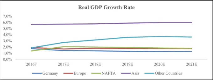
the core question is if the emerging economies like China and India are able to compensate the lost potential of current crisis markets like Russia or Brazil. In addition, one needs to evaluate the development of so far stable markets like the U.S., the Eurozone and the stagnating Japan. According to the IMF (2016), the real GPD growth for Conti’s current major market Germany is expected to continuously decline from 1,7% (FY16) to 1,2% (FY21). Europe as a whole is assumed to decline from 1,9% (FY16) to 1,7% (FY21). Contrariwise, NAFTA will increase from 1,4% (FY16) to 1,8% (FY21) and Asia from 5,7% (FY16) to 6% (FY21) (Figure 1).

(29)

17

Figure 1: Real GDP Growth Rate (Source: IMF, 2016)

Since the company’s sales are reported on a nominal basis, one needs to estimate the inflation rate in addition to the real GDP growth rate. It is expected that the inflation rates within

Ger-many, Europe and NAFTA will rise after FY16 from approx. 1% to 2% in FY21 (Figure 2). Asia will slightly increase from 3% (FY16) to 3,6% (FY21) (IMF, 2016).

Figure 2: Inflation Rate (Source: IMF, 2016)

Besides the mentioned aspects, Conti’s divisions are highly sensitive to the development of raw material prices. For the Automotive division, those are mainly steel, copper and aluminium. For the Tire as well as the ContiTech division, those are natural rubber, Brent oil, butadiene as well as styrene. Except for stainless steel, which price stayed stable, it can be said that all of the named raw material prices sharply decreased since 2011 and consequently improved Conti’s margins (Continental AR, 2015). The World Bank (2016) estimates metal prices to rise by 4% in 2017 after a further 9% drop in 2016 due to tightening supplies. Oil prices are expected to

0,0% 1,0% 2,0% 3,0% 4,0% 5,0% 6,0% 7,0%

2016F 2017E 2018E 2019E 2020E 2021E

Real GDP Growth Rate

Germany Europe NAFTA Asia Other Countries

0,0% 2,0% 4,0% 6,0% 8,0%

2016F 2017E 2018E 2019E 2020E 2021E

Inflation Rate

(30)

18 average at 55$/bbl in 2017, compared to an average of 53$/bbl in 2016. In November 2016, the OPEC reached an agreement for the first production oil cuts since eight years which should further increase the price (Bloomberg, 2016).

3.2 Demand Side Analysis

IHS Automotive (2016) estimates that Light Vehicle (LV) sales growth in Germany will ac-celerate from 1,5% (2017) to 3,9% (2021). Europe will be rather unstable with a growth of 3,4% in 2016 up to 5,9% in 2018 to 2,6% in 2021. NAFTA sales will even decline from 2018 onwards. The Asian sales growth rate will increase from 2,2% (2016) to 5,5% (2017) and sub-sequently decline to 3,6% (2021) (Figure 3).

Figure 3: LV Sales Growth Rate (Source: IHS Automotive, 2016)

Besides a globally increasing demand for vehicles, the demand side is affected by various new disruptive trends. If Conti will successfully align to those factors, they should offer great growth potential but are also connected with high investments. In detail, those trends are autonomous

driving, electrification of the car, connectivity/digitalization as well as shared mobility

(KPMG, 2016; Mohr & Kaas, 2016).

Autonomous driving is the capability of a vehicle to move from Point A to Point B without

any interaction with the driver. Even though the establishment of autonomous driving is not expected until 2030 (KPMG, 2016; Mohr & Kaas, 2016), a stepwise increase of car “intelli-gence” features is assumed to be the first move towards this vision (Hirsch et al., 2015; Hirsch, Jullens, Singh, & Wilk, 2016).

-10,0% -5,0% 0,0% 5,0% 10,0% 15,0%

2016F 2017E 2018E 2019E 2020E 2021E

LV Sales Growth Rate

(31)

19 Due to eco-friendly legislations, the electrification of the car will become another important aspect (KPMG, 2016; Mohr & Kaas, 2016). According to Hirsch et al. (2016), this does not come with a full electrification of the car but just a partial one combined with the simultaneous increase of the efficiency of combustion engines.

Considering KPMG’s (2016) global automotive executive survey, connectivity/digitalization has been identified as the main trend for the next few years. A specific buzzword associated with this topic is the “Internet of Things”, meaning that the intelligent car of tomorrow is able to communicate automatically with various objects in its environments. This might be for both safety and entertainment reasons (Mohr & Mueller, 2013; Mohr & Kaas, 2016).

Another emerging trend will be shared mobility, resulting in an increasing use of on-demand car solutions. The main reason for this development is the ongoing urbanization and the rise of so called megacities. The currently most quoted example in this category might be the applica-tion “Uber” (Hirsch et al., 2016; Mohr & Kaas, 2016).

3.3 Supply Side Analysis

The automotive industry consists of raw material suppliers, 1st_{tier and 2}nd_{tier suppliers, OEMs}

as well as dealers (Figure 4). Conti itself can be described as a tier 1 supplier for mainly all major OEMs like Daimler AG, Fiat-Chrysler, Volkswagen or General Motors. Moreover, it delivers tires to the end customer market and is providing elastomer solutions through its Con-tiTech division (Continental AR, 2015).

(32)

20 Simultaneously to the demand side, the supply side will incur some major changes in the future. Those can be described as pressure for efficiency, market entry of new players as well as

strategic partnerships (Hirsch et al., 2016; Mohr & Kaas, 2016).

The increasing cost pressure and the therewith related pressure for efficiency forces all players along the value chain to continuously improve their operations (Hirsch et al., 2015; Hirsch et al., 2016).

Additionally, the market entry of new players, mostly active in the technology industry, will force a transformation of the industry (Hirsch et al. 2016; Mohr & Kaas, 2016). Since techno-logical knowledge represents one of the core capabilities for staying competitive in the future, firms like Tesla, Google or Apple are already working on projects like autonomous driving (Painter, 2016).

As a response to the above-mentioned factors, strategic partnerships between incumbents and new market entrants will become more important (Hirsch et al. 2015; Mohr & Kaas, 2016). A recent example is the negotiation of Apple with Daimler and BMW to cooperate on the devel-opment of the iCar, which was nonetheless rejected by the two carmakers (Reiche, 2016). Due to the mentioned aspects, Conti’s margins are presumed to be pressured in the close future. This is because of higher expenses (e.g. new investments in R&D) and the fact that the company has to operate on lower margins because of higher competition.

(33)

21

4 Internal Analysis

Continental AG, located in Hannover, Germany, is one of the three biggest automotive compo-nent suppliers in the world (Automotive News, 2013; Statista, 2016a). The company was founded and went public in 1871. In the end of FY15, it employed 207.899 workers at more than 430 subsidiaries in 55 countries. Conti had sales of roughly MEUR39.232 and a net income of MEUR2.727 (Continental AR, 2015).

4.1 Divisions

The group is subdivided into a Chassis & Safety, a Powertrain, an Interior, a Tire as well as a ContiTech division. The first three are summarized to a division called Automotive since they are all involved in the provision of components for OEM manufacturers. The last two are sum-marized to a Rubber division. The five divisions also contain various subdivisions that are not specifically described within the following but listed in the subsequent figure (Continental AR, 2015).

(34)

22 The Chassis & Safety division provides active and passive technologies that enable a better safety, a higher comfort as well as an improved convenience. Its current aim is to offer solutions which focus on the vision of autonomous driving (Continental AR, 2015).

The Powertrain division produces all kinds of powertrain components with the goal of making driving more environmentally compatible. Due to the new environmental legislations, men-tioned before, electrified driving systems are a central issue of the division (Continental AR, 2015).

The Interior division focuses onto information management between the driver, passenger, mobile devices as well as the vehicle. Therefore, connectivity/digitalization is the central issue of the division (Continental AR, 2015).

In the global automotive supplier ranking, Conti has always been underneath the top three sup-pliers in recent years (Statista, 2016a). Its strong competitive position stems from its long-term relationships with OEMs, to which 72% of its FY15 year sales accounted as well as its pressure for innovation (Pearson & Peterc, 2014). In 2015, Conti acquired the German software devel-oper Elektrobit Automotive to strengthen its position in the technology segment. Historically, the Automotive division had a stable EBITDA Margin with an average of 12,3%, which none-theless dropped in Q3 of FY16 to 5%. This sharp decline is mainly attributable to one-time cost effects like cartel penalty provisions. Historically, CAPEX/Sales remained stable at 5,3% (av-erage). This leads to the question if the company will rise this ratio to adapt to the mentioned industry trends (e.g. investments in software) and if the EBITDA Margin will be further pres-sured (Continental AR, 2015; Continental IR, 2016) (Appendix I–Appendix II).

The Tire division sells tires for passenger cars & light trucks, commercial vehicles as well as two-wheelers (Continental AR, 2015). According to Statista (2016), Continental is the fourth biggest tire producer worldwide behind Bridgestone, Michelin and Goodyear. In FY15, it was able to achieve a record EBITDA Margin of 25,1%, mainly due to low raw material prices, full production capacity utilization as well as through its strong competitive position that is because of its brand and its high-quality products (Spina, 2016). In FY16 (Q1–Q3), it even increased to an average of 26,4%. With a ROCE of 39,2%, the division has the highest profitability measure of the whole tire industry (Continental AR, 2015; Continental IR, 2016) (Appendix I–Appendix II).

(35)

23 Through the acquisition of Veyance in FY15 for MEUR1.400, ContiTech strengthened its po-sition as the world’s leading supplier of non-tire elastomer applications before Bridgestone and Freudenberg. Fifty percent of the final customers are located within the automotive industry and the other 50% in various industries beyond the automotive industry (Continental AR, 2015). The downside effect of the Veyance acquisition is the fact that ContiTech’s EBITDA Margin fell by 3,5% from 14,4% (FY14) to 10,9% (FY15) due to acquisition-related costs. Another fact that pressured the company’s margins is the deterioration of the oil, gas and mining industry, which accounts for 25% of the division’s sales (Spina, 2016). Nonetheless, the EBITDA Margin is currently improving and was in the first three quarters of 2016 already at an average of 13,4% again. Another negative side effect of the acquisition is the increase of the NWC from 15,9% of sales (FY14) to 17,7% of sales (FY15) (Continental AR, 2015; Continental IR, 2016) (Ap-pendix I–Ap(Ap-pendix II).

4.2 Corporate and Financing Strategy

„Highly developed, intelligent technologies for mobility, transport and processing make up our world. We want to provide the best solutions for each of our customers in each of our markets (Continental Vision, 2016).” To achieve these long-term goals, Conti developed seven

strate-gic dimensions (Continental AR, 2015). 1. Value creation

2. Regional sales balance 3. Top market position

4. In the market for the market 5. Balanced customer portfolio 6. Technological balance 7. Great people culture

With this seven pillars, Conti tries to respond to the current industry trends. Those are, accord-ing to its opinion, digitalization, urbanization, automated drivaccord-ing as well as electrification. This is in line with the identified trends of the automotive industry. As a defined number, Conti wants to achieve more than MEUR50.000 of sales in 2020 that implies a CAGR of 5%. The

(36)

24

4.3 Share Performance

Since its foundation in 1871, Conti’s share is listed. It has been a continuous member of the DAX, but was reclassified two times, namely in 1996 and 2008, to the MDAX. The share is traded in Frankfurt, Hannover, Hamburg, Stuttgart and OTC in the U.S. Just common stock is available (Continental AR, 2015). The performance of the share price is summarized in the subsequent figure. Since 31st_{October 2011, it has been rising from EUR54 up to EUR229 at its}

peak. Currently, it is at EUR182 (12th_{December 2016).}

Figure 6: Share Price Performance (Source: Thomson Reuters Eikon)

4.4 Shareholder Structure

In 2008, the Schaeffler family, owners of the Schaeffler AG, tried to acquire Conti in a hostile takeover. Currently, the family holds 46% of the company’s stock and therefore Conti is re-garded as a sister enterprise of Schaeffler. The acquisition was considered highly speculative and due to the stock market crash, initiated by the Lehman Brothers collapse in 2008, Schaeffler almost went bankrupt. Even though Conti is not under its full control, the Schaeffler family can exercise significant influence. This had been witnessed by the announcement of Elmar Degen-hart to CEO in 2009 (Jungbluth, 2015). The other 54% of the shares are free floating, whereby BlackRock (3,0%), Deutsche Asset Management (1,8%) and Norges Bank Investment Man-agement (1,4%) are currently the biggest investors (Thomson Reuters Eikon).

0 50 100 150 200 250 31 -Oc t-2 01 1 31 -De c-2 01 1 29 -F eb -2 01 2 30 -Ap r-2 01 2 30 -Ju n-2 01 2 31 -Au g-2 01 2 31 -Oc t-2 01 2 31 -De c-2 01 2 28 -F eb -2 01 3 30 -Ap r-2 01 3 30 -Ju n-2 01 3 31 -Au g-2 01 3 31 -Oc t-2 01 3 31 -De c-2 01 3 28 -F eb -2 01 4 30 -Ap r-2 01 4 30 -Ju n-2 01 4 31 -Au g-2 01 4 31 -Oc t-2 01 4 31 -De c-2 01 4 28 -F eb -2 01 5 30 -Ap r-2 01 5 30 -Ju n-2 01 5 31 -Au g-2 01 5 31 -Oc t-2 01 5 31 -De c-2 01 5 29 -F eb -2 01 6 30 -Ap r-2 01 6 30 -J un -2 01 6 31 -Au g-2 01 6 Oc t-2 01 6

(37)

25

5 Valuation

The subsequent chapter introduces the drafted financial model of the author as a basis for an investment decision.

5.1 Methodology

The SOP approach, applying a DCF analysis (with WACC) as well as multiples, has been cho-sen as the most suitable valuation methodology. This is due to the fact that Conti’s divisions are heterogeneous in their business activities (Chapter 4.1.), making it necessary to distinct between certain risk parameters (e.g. beta or ERP).

For the purpose of this thesis, the author differentiated between the Automotive division, the

Tire division and the ContiTech division. The Automotive division was not further subdivided

into its three subdivisions (Figure 5), because it is presumed to be too difficult to find adequate peers just active within this specific kind of businesses.

The financial reporting scope and the quality is suitable for the mentioned kind of valuation since Conti reports various fundamentals like sales, EBIT, D&A, NWC as well as CAPEX by division (Appendix I–Appendix II).

The WACC is computed by division, whereby it is differentiated between two scenarios. First, it is assumed that the industry’s median represents the target capital structure for which the company should aim. Second, the company’s current capital structure is expected to be the optimal one. For the beta computation, the industries’ betas (peer group betas) are used and re-levered at the above-mentioned ratios. This basically delivers six betas, used to compute six costs of equity as well as six WACCs.

The multiples valuation uses the same peer groups as composed for the WACC and applies asset trailing as well as asset leading multiples (FY16 and FY17). No equity multiples are used, because the reporting quality does not enable an appropriate application of this approach. In detail, this is due to the fact that earnings are not reported by division and some assets/liabilities are not allocated to any specific division.

Additionally, a scenario analysis runs six different scenarios, including a high-growth or a low-growth scenario. One of them also performs an APV valuation, presuming a stepwise change in the company‘s capital structure. Within the single scenarios, the WACC is differentiated

(38)

26 +/– 0,5%. Basically, it should enable the reader to gain an overview of the range the PPS could take under certain ceteris-paribus considerations.

After the determination of the final PPS, it is evaluated how much an investor could maximally lose (and gain) per day when purchasing Conti’s stock. This is done through a Value at Risk (VaR) analysis, using a Monte Carlo simulation.

5.2 Financial Forecasts

In the following section, the financial forecasts by division are presented. Appendix

III–Ap-pendix V contains all of the historical data as well as the specific forecasts. 5.2.1 Sales

The Automotive group is Conti’s biggest division according to sales and consequently of major importance. Currently, it achieves the majority of its sales in Europe, especially Germany, whereas the division is stepwise increasing its share in the NAFTA and in Asia (Table 4) (Con-tinental Facts & Figures, 2015).

Table 4: Automotive – Sales by Region (Source: Continental AR, 2015)

Conti expects high growth (25%–100%) for gasoline particulate filters, switchable coolant and oil pumps as well as lane departure warning systems. Medium growth (15%–24%) is expected for turbochargers, start-stop systems as well as battery propulsion systems. This is attributable to the mentioned change to environmentally friendly powertrains. Tackling this issue, Conti is already able to reduce CO2 emissions by 20%–25% with its hybrid electric vehicle or by 15%– 20% with compressed natural gas. As a result, it already holds various competitive products in its portfolio. Also the trend of connectivity/digitalization is taken into consideration with vari-ous applications like tire pressure monitoring systems (environment), hands-free telephony (safety) or intelligent transport systems (Continental Facts & Figures, 2015). The Advanced Driver Assistance System (ADAS) is another important product in Conti’s portfolio that is cur-rently gaining high importance (Pearson & Peterc, 2014).

Automotive

Year 2010 2011 2012 2013 2014 2015 Average

Germany 29,0% 28,0% 26,7% 25,7% 25,0% 23,7% 26,3%

Europe (excluding Germany) 26,3% 26,7% 23,7% 23,0% 23,3% 23,0% 24,3%

NAFTA 19,3% 19,7% 22,7% 23,0% 22,7% 25,7% 22,2%

Asia 21,0% 21,7% 23,7% 25,0% 25,7% 26,0% 23,8%

(39)

27 Conti’s automotive sales are expected to be influenced by the current economic cycle, measured on a nominal basis, and the increase of global vehicle sales. For the FY16 growth, the current interim growth rates (Q1–Q3) are mainly taken into consideration. All of the inputs are weighted according to Conti’s sales exposure to its various geographical business regions. Be-cause of the strong competition within the automotive segment, it is presumed that Conti is highly exposed to the current economic cycle (40%) and to the vehicle sales growth (60%). The author holds the opinion that Conti will grow weaker than the nominal GDP growth rate but more than the global vehicle sales growth rate due to the fact that, through its innovative prod-ucts and long-term OEM relationships, Conti should exceed the global vehicle sales growth and gain new market share. The growth rate is presumed to stabilize for all divisions after a fore-casting horizon of six years (Table 5). The whole computation can be withdrawn from Appen-dix VI.

Table 5: Automotive – Sales Forecast (Source: Own Calculations)

For the Tire division, increasing safety and environmental regulations around the globe should further support Conti in growing its sales. More specifically, this is the pressure for using winter or environmentally friendly labelled tires. Conti Tire has its strongest presence in Europe, spe-cifically Germany. In Europe, Conti shares approx. 50% of the total market share with Good-year and Michelin. Sales in NAFTA have recently been increasing. The current weak exposure to Asia results from the fact that Asian suppliers like Bridgestone or Hankook are already oc-cupying the market (Continental Facts & Figures, 2015) (Table 6).

Table 6: Tire – Sales by Region (Source: Continental AR, 2015)

The Tire growth rate is based on the same sales drivers as the Automotive division, except that also the tire replacement growth rate (historical CAGR of the industry) is taken into considera-tion. The author expects Tire to be less influenced by the economic cycle (20%) and more by

Automotive

Amounts in MEUR 2015 2016F 2017E 2018E 2019E 2020E 2021E

Sales 23.565 24.340 25.253 26.271 27.285 28.207 29.193

Sales YoY Growth (%) 3,3% 3,8% 4,0% 3,9% 3,4% 3,5%

Tire

Year 2010 2011 2012 2013 2014 2015 Average

Germany 19,0% 19,0% 18,0% 17,0% 17,0% 15,0% 17,5%

NAFTA 21,0% 20,0% 24,0% 23,0% 24,0% 27,0% 23,2%

Asia 6,0% 6,0% 8,0% 9,0% 8,0% 9,0% 7,7%

(40)

28 the global vehicle sales growth rate (70%) as well as slightly by the tire replacement growth rate (10%). As a result, the Tire division will post a weaker growth than Automotive. This is due to the assumption that there will be no rapid industry disruption, as expected for the auto-motive segment, resulting in only minimal space to create new market share through innovation (Spina, 2016) (Table 7). Nevertheless, because of the new environmental legislations and Conti’s high-quality rubber products (from which its competitive advantage results), the tire growth rate should be slightly above the global LV sales growth rate. Appendix VII contains the whole computation.

Table 7: Tire – Sales Forecast (Source: Own Calculations)

ContiTech’s sales by region are, like for the other divisions, scattered with a main focus on

Europe, especially Germany. With the recent Veyance acquisition, Conti tried to increase its exposure to NAFTA as well as to Southern America (Continental AR, 2015) (Table 8).

Table 8: ContiTech – Sales by Region (Source: Continental AR, 2015)

It is assumed that ContiTech‘s growth rate is solely based on the nominal GDP growth rate, except in FY16 where the current interim growth rates are taken into consideration. In addition, a discount of 2% is applied to the nominal GDP growth rate, to account for the fact that the group will not grow as strong as the overall economy. This is mainly due to the fact that Conti’s rubber products do not offer enough opportunities to create higher market share through inno-vation (Spina, 2016) (Table 9) (Appendix VIII).

Table 9: ContiTech – Sales Forecast (Source: Own Calculations)

Tire

Sales 10.388 10.667 10.966 11.350 11.740 12.049 12.365

Sales YoY Growth (%) 2,7% 2,8% 3,5% 3,4% 2,6% 2,6%

ContiTech

Year 2010 2011 2012 2013 2014 2015 Average

Germany 38,0% 16,0% 34,0% 33,0% 33,0% 24,0% 29,7%

NAFTA 7,0% 30,0% 10,0% 12,0% 14,0% 26,0% 16,5%

Asia 14,0% 8,0% 16,0% 16,0% 17,0% 17,0% 14,7%

Other Countries 7,0% 12,0% 8,0% 8,0% 5,0% 8,0% 8,0%

ContiTech

Sales 5.279 5.372 5.525 5.664 5.809 5.958 6.110

(41)

29

5.2.2 EBITDA Margin

Even though the consolidated income statement of Conti is reported according to the function of expense-method, the single divisions just report profit metrics like EBIT and EBITDA. Con-sequently, expenses like COGS, SGA and R&D cannot be appropriately separated and there-fore, the forecasts have to be done by applying margins. As a result, EBITDA Margins are forecasted for the single divisions.

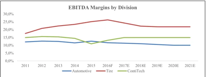
Within the Automotive Division, the EBITDA Margin has been stable around an average of 12,3% between FY11 and FY15. It is expected that the margin will be at 11,6% in FY16, which is the median of the first three quarters of FY16. This metric is used to exclude the Q3 outlier (FY16) which is just at 5,0%, mainly because of one-time effects like cartel penalty provisions. In FY17 and FY18, it will slightly decline by 0,3%. From FY20 onwards, it will stay stable at 10%. The decline is attributable to increasing raw material prices (World Bank, 2016), the mar-ket entrance of new technology players and increasing R&D costs (investments to adapt to industry trends) that will all pressure Conti’s margins (Figure 7).

The EBITDA Margin at the Tire Division has continuously improved from 17,5% in FY11 to 25,1% in FY15. In FY16, the interim median is even at 26,2%. Nonetheless, it is assumed that raw material prices (especially oil) will increase (World Bank, 2016) and that the current ca-pacity utilization cannot be kept at record levels. As a consequence, the EBITDA Margin should stepwise decrease by 2% each year, from 26,2% in FY16 to 22,2% in FY18. From FY19 on-wards, it will be stable at 21,8% (FY11-FY15 average). Due to Conti’s strong competitive ad-vantage in the Tire business, it is not presumed to fall below that level (Figure 7).

Before 2015, the EBITDA Margin of ContiTech has been stable around an average of 15,1% but dropped to 10,9% in FY15 (due to the Veyance acquisition). As the EBITDA Margins within the FY16 interim reports are already ascending to the former levels (13,2% median in Q1–Q3), it is presumed that the margin will rebound and stay stable at the 5-years median from FY17 onwards, since the company is expected to successfully handle all the acquisition issues (Figure 7).

(42)

30

Figure 7: EBITDA Margin by Division (Source: Own Calculations) 5.2.3 D&A

In the subsequent sections, D&A, CAPEX as well NWC are measured as a percentage of sales to construct the forecasts. For the D&A forecasts, impairment is excluded, because extraordi-nary effects are not taken into consideration.

For the Automotive division, D&A/Sales has been decreasing from 6,5% in FY11 to 4,1% in FY15. As CAPEX/Sales is expected to increase due to higher investments to adapt to the current industry trends, also D&A will step-by-step increase from 4,1% (FY16–FY17) to 5% (FY18– FY21).

Contrary to the Automotive division, D&A/Sales has been increasing within the Tire division from 3,8% (FY11) to 5% (FY15). Nevertheless, no higher investments are expected for the Tire segment and that is why D&A/Sales will stay stable at the FY15 ratio.

ContiTech’s D&A/Sales ratio has been stable in the past, except a recent sharp rise from 3,1%

(FY14) to 7,7% (FY15). This is mainly related to an impairment loss for the Conveyor Belt Group of MEUR72 and an acquisition-related increase of D&A. For FY16, the interim median of Q1–Q3 is used (5,5%) and in FY17 a decline of 1,5% to 4% is presumed. Afterwards (FY18– FY21), the ratio will stay at the historical median (applied to exclude the FY15 outlier) of 3% (Figure 8). 0,0% 5,0% 10,0% 15,0% 20,0% 25,0% 30,0%

2011 2012 2013 2014 2015 2016F 2017E 2018E 2019E 2020E 2021E

EBITDA Margins by Division