MARIANA DIAS
ALMEIDA
COMUNIDADES SUPRABENTÓNICAS DO
MEDITERRÂNEO BATIAL: INFLUÊNCIA DE
FACTORES AMBIENTAIS NA DIVERSIDADE E
ESTRUTURA DA COMUNIDADE
DEEP-SEA SUPRABENTHOS ACROSS THE
MEDITERRANEAN: THE INFLUENCE OF
ENVIRONMENTAL DRIVERS ON BIODIVERSITY AND
COMMUNITY STRUCTURE
MARIANA DIAS
ALMEIDA
COMUNIDADES SUPRABENTÓNICAS DO
MEDITERRÂNEO BATIAL: INFLUÊNCIA DE
FACTORES AMBIENTAIS NA DIVERSIDADE E
ESTRUTURA DA COMUNIDADE
DEEP-SEA SUPRABENTHOS ACROSS THE
MEDITERRANEAN: THE INFLUENCE OF
ENVIRONMENTAL DRIVERS ON BIODIVERSITY AND
COMMUNITY STRUCTURE
Tese apresentada à Universidade de Aveiro para cumprimento dos requisitos necessários à obtenção do grau de Doutor em Biologia, realizada sob a orientação científica da Professora Doutora Maria Marina Ribeiro Pais da Cunha, Professora Auxiliar do Departamento de Biologia da Universidade de Aveiro e co-orientação do Doutor Joan Baptista Claret Company, Investigador Sénior do Institute of Marine Sciences, Espanha e do Doutor Nikolaos
Lampadariou, Investigador do Hellenic Center for Marine Research, Grécia.
Apoio financeiro da Fundação para a Ciência e a Tecnologia (FCT) e do Fundo Social Europeu (FSE) no âmbito do III Quadro Comunitário de Apoio, bolsa de referência (SFRH/BD/69450/2010), e dos projetos: - DESEAS (EEC DG Fisheries Study Contract
2000/39)
- RECS (REN2002-04556-C02-01) - BIOFUN (CTM2007-28739-E)
- PROMETEO (CTM2007-66316-C02/MAR) - DOSMARES (CTM2010-21810-C03-03/MAR).
o júri
presidente Professor Doutor Amadeu Mortágua Velho da Maia Soares Professor Catedrático da Universidade de Aveiro
Professor Doutor Pablo Sànchez Jerez Professor Titular, Universidade de Alicante, Espanha Professora Doutora Magdalena Blazewicz Professora Associada, Universidade de Lodz, Polónia
Professora Doutora Maria Marina Pais Ribeiro da Cunha Professora Auxiliar, Universidade de Aveiro (orientadora)
Doutora Ana Margarida Medrôa de Matos Hilário Equiparada a Investigadora Auxiliar, Universidade de Aveiro
agradecimentos O trabalho desenvolvido apenas foi possível devido a pessoas que contribuíram para a minha formação académica e pessoal, às quais gostaria de agradecer, em particular:
À Professora Doutora Marina Cunha pela excelência científica, apoio e bom humor, e pela oportunidade de fazer parte da equipa do LEME.
I would like to thank to my co-supervisors Dr. Nikolaos Lampadariou and Dr. Joan Company for the support in various aspects of this project, ready availability and the chance to participate in oceanographic campaigns. Thanks to the members of the J.B. Company Lab, N. Lampadariou Lab and D. Martin Lab.
To taxonomy expert on peracarid crustaceans Dr. Wanda Plaiti from the Hellenic center for Marine Research (Crete, Greece); on decapods Dr. Pere Abelló from the Institute of Marine Sciences (Barcelona, Spain); on mysids Dr. Inmaculada Frutos from Center of Natural History, University of Hamburg (Hamburg, Germany) an on tanaids to Patricia Esquete from CESAM. À Ascensão Ravara, Luciana Génio, Clara Rodrigues e Rui Vieira pelas identificações de não crustáceos e Fábio Matos pela ajuda informática. E a todos os colegas e amigos do LEME pelo bom ambiente e partilha dos dias (e por muitas mais coisas).
Ao Mário. Aos meus pais, que não puderam estudar.
A título introdutório relativamente a este trabalho: Quem dá o que tem, a mais não é obrigado (Provérbio Português)
palavras-chave Canhões submarinos; Mar Mediterrâneo; Comunidades suprabentónicas; Biodiversidade; Mar profundo; Oligotrofia
resumo O mar Mediterrâneo batial apresenta características homeotérmicas (~14°C) e um gradiente de oligotrofia, que se acentua de oeste para este, de grande interesse para estudos de distribuição da fauna em mar profundo.
Encontram-se também presentes outras condições específicas, de que são exemplos os processos oceanográficos e topográficos, que determinam variações ambientais nas suas diferentes regiões. Em particular, destaca-se o noroeste do Mediterrâneo cuja influência de canhões submarinos favorece uma maior produtividade e pressão antropogénica, que se traduz numa relevante atividade de pesca de arrasto em mar profundo. Embora pouco investigada, a macrofauna que habita acima do sedimento, designada por suprabentos, é uma componente importante da fauna bentónica com relevância nas cadeias tróficas de mar profundo. Neste contexto, foram estudadas as comunidades suprabentónicas ao longo de um gradiente oligotrófico (600-3000m; região oeste; mar Baleárico; centro, mar Jónico; este, Sul de Creta) e num canhão submarino e talude adjacente (400-2250m; noroeste do Mediterrâneo, mar da Catalunha) com o objetivo de caracterizar a biodiversidade, abundância e a estrutura da comunidade em relação com as variáveis ambientais. Em cada um dos locais, obtiveram-se amostras em três níveis da coluna de água acima do sedimento (10-50cm, 55-95cm e 100-140cm), de modo a caracterizar a distribuição vertical da macrofauna suprabentónica.
Este estudo identificou 232 taxa e 18 grupos tróficos, evidenciando-se os anfípodes e os cumáceos com um maior número de espécies. Os grupos mais abundantes foram os anfípodes, sobretudo predadores de zooplâncton, e os misidáceos seguidos dos isópodes, ambos maioritariamente omnívoros. A análise da distribuição vertical da macrofauna revelou uma diminuição acentuada na sua densidade do nível mais próximo do sedimento (10-50cm) para os níveis superiores. A estrutura da comunidade apresentou variações relacionadas com diversos fatores ambientais tais como, a quantidade e qualidade do alimento, o hidrodinamismo (associado a condições típicas do canhão) e a estrutura das massas de água. Os resultados mostram que as densidades apresentaram uma grande amplitude (3.5-538.9 ind.100m-2) tendo os valores máximos sido registados no canhão de Blanes e no talude adjacente a cerca de 900m de profundidade. O número de espécies e o índice de diversidade de Shannon variaram entre os 21 e 84 e entre 1,28 e 3,35, respetivamente, tendo sido registada a menor diversidade no canhão submarino. Ao longo do gradiente de oligotrofia, de oeste para este, verificou-se um decréscimo das densidades e do número de espécies e constatou-se uma diminuição da abundância relativa de grupos que se alimentam no sedimento, em paralelo com o aumento da abundância relativa de grupos que se alimentam na coluna de água. Estes resultados foram associados a uma diminuição da matéria orgânica nos sedimentos da área mais oligotrófica. A distribuição estratificada variou ao longo do
gradiente longitudinal, o que parece refletir a dinâmica das espécies (e.g. mobilidade, capacidade de dispersão, alimentação), as diferentes respostas das espécies à variabilidade nas condições abióticas, possíveis barreiras à dispersão e ao gradiente de oligotrofia, resultando em valores elevados de β-diversidade. A noroeste, no canhão de Blanes, a estrutura da comunidade parece ser condicionada pela maior quantidade e diversidade de fontes de matéria orgânica indicada pela presença de predadores no sedimento e de detritívoros no talude adjacente. Nas zonas do canhão mais próximas da influência terrestre, a estrutura e a biodiversidade da macrofauna
suprabentónica parecem estar relacionadas com a variabilidade temporal das condições hidrodinâmicas, em particular, no aumento da intensidade de correntes e de fluxo de partículas que ocorre no outono e no inverno
(descargas do rio e tempestades). Nestas condições, verificou-se o aumento da densidade e a redução da biodiversidade, possivelmente devido a uma maior presença de omnívoros com elevada mobilidade (ex. misidáceos). No talude adjacente, caracterizado por menor perturbação natural e maior qualidade de matéria orgânica de origem pelágica, a comunidade reflete uma diversidade elevada, em especial, na primavera. A maior profundidade, observou-se uma diversidade similar no canhão e no talude, provavelmente devido a condições de inferior perturbação natural e menor influência da ação do canhão. No entanto, após a ocorrência de um processo energético de grande intensidade, como o efeito de cascata de massas de água de elevada densidade (ex. 2012), verificou-se um aumento considerável do número de espécies e das densidades no canhão e no talude. Este aumento pode dever-se a um incremento de matéria orgânica fresca no talude inferior e na bacia do Mediterrâneo. Apesar da resiliência das comunidades
suprabentónicas, a sua diversidade parece ser afetada pela elevada e continuada perturbação causada pela pesca de arrasto.
Concluindo, neste trabalho existem evidências de que as diferentes regiões analisadas apresentaram elevada variabilidade na composição, estrutura e biodiversidade, que se atribui à heterogeneidade de grupos tróficos e modos de vida do suprabentos. Os valores de β-diversidade observados foram atribuídos à disponibilidade de alimento, heterogeneidade do habitat e perturbação natural. Os resultados deste estudo evidenciam a necessidade de considerar os mesmos elementos faunísticos na composição teórica da fauna que vive na interface coluna água/sedimento para comparação com outras regiões. Estudos de auto-ecologia e interações bióticas e, finalmente, a necessidade de amostragem replicada, são também aspetos a considerar para uma melhor compreensão das comunidades de suprabentos.
Recomenda-se, por fim, dada a relevância funcional das comunidades suprabentónicas, a inclusão deste compartimento bentónico em futuros estudos focados no funcionamento dos ecossistemas de mar profundo.
keywords Submarine canyons; Mediterranean Sea; Suprabenthos; Biodiversity; Deep-sea; Oligotrophy
abstract The Mediterranean Sea is characterized by homeothermia (~14ªC) and a gradient of increasing oligotrophy from west to east which makes it of particular interest to study distribution patterns of deep-sea fauna. Particular oceanographic processes and topographic characteristics vary in different regions. The northwestern Mediterranean, where the shelf is deeply incised by numerous submarine canyons, is typically more productive and it is also subjected to an intense anthropogenic pressure mainly by deep-sea bottom-trawling fisheries.
The suprabenthos, loosely defined as the macrofauna living in the
sediment/water column interface, is an important component of the benthic fauna, with a relevant role in deep-sea food webs, albeit poorly investigated. In this context, suprabenthic assemblages were studied along an oligotrophic gradient (600-3000 m water depths; western region, Balearic Sea; central region, Ionian Sea; eastern region, South of Crete) and in a submarine canyon and adjacent slope (400-2250 m; northwestern Mediterranean Sea, Catalan Sea) aiming to examine their biodiversity, abundance and
community structure in relation to varying environmental conditions. In each sampling site, samples were collected at three water layers above the sediment (10-50 cm; 55-95 cm; 100-140 cm), allowing to characterize the vertical distribution in the close vicinity of the seafloor.
The specimens collected were ascribed to 232 taxa, from which amphipods and cumaceans were the most species-rich groups. Amphipods, mostly predators on zooplankton, followed by mysids and isopods, mostly
omnivores, were the most abundant groups. The analysis of the near-bottom vertical distribution of the suprabenthic fauna showed a marked decreased in densities from the layer closer to the sediment (10-40 cm water layer) to the upper layers. Community structure varied in relation to environmental variables such as food input, hydrodynamic regime, topographic features (e.g. canyon-associated conditions) and properties of the water masses. The general results showed high variability in densities (3.5-538.9 ind.100 m-2) with maximum values registered in the Blanes Canyon and adjacent slope at 900 m depth. The number of species and the Shannon biodiversity index varied from 21 to 84 and from 1.28 to 3.35, respectively, with the lowest biodiversity observed in the canyon.
Along the longitudinal gradient, densities and number of species decreased, the relative abundance of animals relying on food sources from the sediment decreased in parallel with an increase in the relative abundance of animals feeding on the water column. These results likely reflect the low organic matter input to the sediments in the more oligotrophic region. The near-bottom vertical distribution of the fauna changed along the longitudinal gradient, which may be associated to the functional traits of the species
(e.g. motility, dispersion capability, feeding mode), to the different responses of individual species to changing abiotic conditions, the occurrence of topographic barriers and to the oligotrophy. These changes in the
composition of the suprabenthic assemblages maintained similar values of α-diversity across the longitudinal/oligotrophy gradient, but resulted in high turnover (β-diversity).
In the northwestern region the community structure appeared to be driven by the quantity and quality of food sources, revealed by the presence of surface predators in the Blanes Canyon and adjacent slope and also detritivores in the latter environment. In the canyon head and upper reaches, the
community structure and biodiversity appeared to be driven by the temporal variability in hydrodynamic conditions with increased intensity of currents and particle fluxes in autumn and winter (river discharges, storms). Under
disturbance conditions, densities increased and biodiversity decreased due to the dominance of omnivores with high motility (e.g. mysids). In the slope, the assemblages appeared to respond to the lower particle fluxes but higher quality of the predominantly pelagic organic input, by showing an increased biodiversity, particularly in spring. At deepest sites, biodiversity was similar between canyon and open slope, probably owing to the lower intensity of natural disturbance and lessening of a putative canyon effect. Nevertheless, after the occurrence of high energetic processes, such as a dense shelf cascading event (e.g. in 2012), an important increase in the number of species and densities was observed both in the canyon and slope, probably reflecting the increment of fresh organic matter in the lower slopes and basin. Despite the overall high resilience of suprabenthic assemblages, they were affected by high and continued trawling disturbance.
In conclusion, this Thesis showed evidence of highly variable patterns in the composition, biodiversity and structure of the suprabenthic assemblages typified by the occurrence of a variety of trophic groups and life styles. High levels of spatial and temporal turnover in species composition was attributed to food availability, habitat heterogeneity and natural disturbance.
In order to improve the knowledge on deep-sea suprabenthos, more studies on its auto-ecology and biotic interactions are needed. Also important to enable biogeographical and even regional comparisons, is to reach a consensus on a standardized terminology and conceptual definition concerning this faunal compartment, as well as to improve the spatial and temporal replication of sampling. Finally, given the important functional role of suprabenthos in marine food webs, it is strongly recommended to include this benthic compartment in future studies focusing on deep-sea ecosystem functioning.
Declaro que esta tese é integralmente da minha autoria, estando devidamente referenciadas as fontes e obras consultadas, bem como identificadas de modo claro as citações dessas obras. Não contém, por isso, qualquer tipo de plágio quer de textos publicados, qualquer que seja o meio dessa publicação, incluindo meios eletrónicos, quer de trabalhos académicos.
i
TABLE OF CONTENTS
SECTION 1.
INTRODUCTION ... 1
1.1 GENERAL BACKGROUND ...3
1.1.1 MAJOR ENVIRONMENTAL CHARACTERISTICS OF THE DEEP SEA ...4
1.1.2 BIODIVERSITY IN THE DEEP SEA: GENERAL CONSIDERATIONS ...8
1.1.3 THE MEDITERRANEAN SEA ...14
1.1.4 SUPRABENTHOS ...29
1.2 OBJECTIVES AND THESIS OUTLINE ...33
SECTION 2.
RESULTS ... 59
2.1 CHARACTERIZATION OF SUPRABENTHIC ASSEMBLAGES FROM THE BATHYAL MEDITERRANEAN SEA ...61
2.1.1 INTRODUCTION ...62
2.1.2 MATERIAL AND METHODS...64
2.1.3 RESULTS AND DISCUSSION ...73
2.2 COMPARISON OF DEEP-SEA CRUSTACEAN SUPRABENTHIC COMMUNITY STRUCTURE AND BIODIVERSITY IN THE WESTERN AND CENTRAL MEDITERRANEAN SEA ... 131
ABSTRACT... 132
2.2.1 INTRODUCTION ... 132
2.2.2 MATERIAL AND METHODS... 134
2.2.3 RESULTS ... 136
2.2.4 DISCUSSION ... 147
2.2.5 CONCLUSIONS ... 150
2.3 BIODIVERSITY PATTERNS OF CRUSTACEAN SUPRABENTHIC ASSEMBLAGES ALONG AN OLIGOTROPHIC GRADIENT IN THE BATHYAL MEDITERRANEAN SEA ... 161
ABSTRACT... 162
2.3.1 INTRODUCTION ... 163
2.3.2 MATERIAL AND METHODS... 165
2.3.3 RESULTS ... 170
2.3.4 DISCUSSION ... 186
ii
2.4 BIODIVERSITY OF SUPRABENTHIC PERACARID ASSEMBLAGES FROM
THE BLANES CANYON REGION (NW MEDITERRANEAN SEA) IN RELATION TO
NATURAL DISTURBANCE AND TRAWLING PRESSURE ... 205
ABSTRACT... 206
2.4.1 INTRODUCTION ... 207
2.4.2 MATERIAL AND METHODS... 209
2.4.3 RESULTS ... 214
2.4.4 DISCUSSION ... 227
2.5 SUPRABENTHIC CRUSTACEAN ASSEMBLAGES SUBJECTED TO HIGH-ENERGY HYDRODYNAMIC EVENTS IN THE BLANES CANYON AND ADJACENT SLOPE (NW MEDITERRANEAN SEA) ... 249
ABSTRACT... 250
2.5.1 INTRODUCTION ... 250
2.5.2 MATERIAL AND METHODS... 253
2.5.3 RESULTS ... 258
2.5.4 DISCUSSION ... 270
2.5.5 CONCLUSIONS ... 275
SECTION 3.
GENERAL DISCUSSION ...287
LIST OF FIGURES
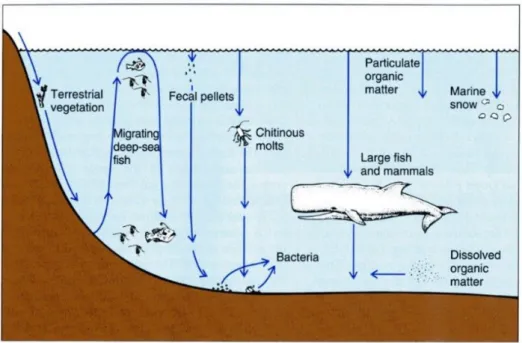
Figure 1.1 Diagrammatic cross section of the ocean floor showing the major topographic features and depth zones. The subittoral zone is not labelled. Modified from Gage and Tyler (1991). ...3Figure 1.2 Schematic representation of the various food sources for the deep-sea. Modified from Nybakken and Bertness (2005). ...7
Figure 1.3 The Mediterranean Basin configuration. Modified from Demirov and Pinardi (2002). ...15
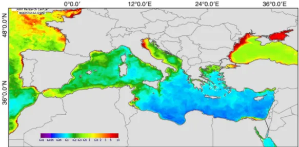
Figure 1.4 Surface chlorophyll-a concentration in the Mediterranean Sea in June 2009, used as a proxy of surface primary production, expressed as mg.m-3. Data was retrieved from the Environmental Marine Information System (EMIS) (http://emis.jrc.ec.europa.eu/emis_1_0.php). ...16
Figure 1.5 Overall water circulation driven by the Atlantic Water. Modified from Millot and Taupier-Letage (2005). ...17
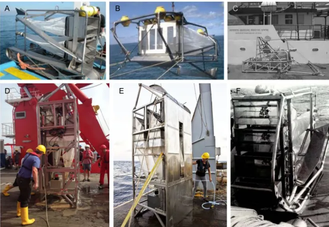
iii Figure 1.6 Submarine canyons of the western Gulf of Lion and the Catalan margin. Valencia Channel (VC) and main rivers opening at short distance from submarine canyon heads are also showed. HC: Herault Canyon. AC: Aude Canyon. PC: Pruvot Canyon. LDC: Lacaze-Duthiers Canyon. CCC: Cap de Creus Canyon. LFC: La Fonera Canyon. BC: Blanes Canyon. ArC: Arenys Canyon. BeC: Besos Canyon. CPC: Can Pallisso Canyon. MC: Morras Canyon. BerC: Berenguera Canyon. FC: Foix Canyon. CC: Cubelles Canyon. TR: Ter River. ToR: Tordera River. LLR: Llobregat River. From Canals et al., 2013...20 Figure 1.7 Scheme representing the three main oceanographic processes driving the NW Mediterranean Sea: dense shelf water cascading (DSWC), offshore convection and eastern storms (the ‘‘three tenors’’). The main water masses are also showed. AW: Atlantic Water; WIW: LIW: Levantine Intermediate Water; WMDW: Western Mediterranean deep water. From Canals et al., 2013. ...21 Figure 2.1.1 Examples of gears used to sample the epibenthic/suprabenthic macrofauna. A: Modified Sanders sledge (Mastrototaro et al., 2010); B: Sorbe sledge (http://www.theseusproject.eu/wiki/Sampling_tools_for_the_marine_environment); C:
TTS sledge (Koulouri et al., 2003); D: EBS sledge
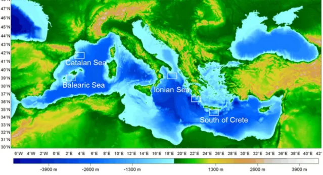
(http://www.oceanblogs.org/so237/2014/12/22/); E: Brenke sledge (http://abyssline.blogspot.pt/2015/03/thats-one-giant-sled-brenke-sledge.html); F: Macer-Giroq sledge (Dauvin et al., 1995). ...63 Figure 2.1.2 Map of the sampling sites. Catalan Sea and Balearic Sea in the western Mediterranean Sea (W), the western and eastern Ionian Sea in the central Mediterranean Sea (C) and South of Crete in the eastern Mediterranean Sea (E) (http://www.unipv.it/cibra/MedBathy%20800.gif). ...65 Figure 2.1.3 3D image of the Blanes Canyon illustrating the main domains in terms of sediment dynamics and sediment transport pathways across the shelf and into the canyon. From Canals et al., 2013. ...67 Figure 2.1.4 Modified version of the Macer-GIROQ sledge. ...71 Figure 2.1.5 Frequent crustacean meiofauna and larvae and non-crustacean groups collected with the Macer-Giroq sledge. A: Copepoda, B: Ostracoda, C: Chaetognatha, D, F: Tunicata, E: Pisces larvae, G: Pteropoda, H: Cephalopoda larvae, I, K: Decapoda larvae, J, M: Pisces, L: Gelatinous taxa. ...72
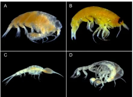
iv Figure 2.1.6 Number of species (A) and individuals (B) of the major taxonomic groups of suprabenthos from all samples taken in the Mediterranean Sea (N1: 10-50 cm, N2: 55-95 cm; N3: 100-140 cm; Total: 10-140 cm). ...74 Figure 2.1.7 Number of trophic groups in the suprabenthos from all samples taken in the Mediterranean Sea (N1: 10-50 cm, N2: 55-95 cm; N3: 100-140 cm; Total: 10-140 cm). EP: water column/epibenthic; SR: seafloor surface; SS: sediment subsurface; mic: microfauna; mei: meiofauna; mac: macrofauna; zoo: zooplankton; fis: fish; Dt: detritus feeder; De: deposit feeder; Su: suspension/filter feeder; Pr: predator; Sc: scavenger; Sp: sectorial parasite; Gr: grazer; Om: omnivorous; U: unknown. ...76 Figure 2.1.8 Specimens of hyperiids collected in the bathyal Mediterranean Sea. A:
Primno macropa B: Vibilia armata; C: Oxycephalidae, D: Phronimidae. ...93
Figure 2.1.9 Specimens of gammarids collected in the bathyal Mediterranean Sea. A:
Bruzelia typical, B: Synchelidium haplocheles, C: Scopelocheirus hopei D: Bathymedon longirostris E: Rhachotropis sp. F: Mediterexis mimonectes. ...94
Figure 2.1.10 Bathymetric ranges of the species of the sub-order Hyperiidea collected in the bathyal Mediterranean Sea. Undetermined specimens are not included. ...94 Figure 2.1.11 Bathymetric ranges of the species of the sub-order Senticaudauta collected in the bathyal Mediterranean Sea. ...94 Figure 2.1.12 Bathymetric ranges of the species of the sub-order Gammaridea collected in the bathyal Mediterranean Sea. Undetermined specimens are not included. ...95 Figure 2.1.13 Specimens of cumaceans collected in the bathyal Mediterranean Sea. A:
Diastyloides serratus, B: Leucon longirostris, C: Platysympus typicus. ...97
Figure 2.1.14 Bathymetric ranges of the cumacean species collected in the bathyal Mediterranean Sea. Undetermined specimens are not included. ...97 Figure 2.1.15 Specimens of isopods collected in the bathyal Mediterranean Sea. A:
Munnopsurus atlanticus, B: Gnathiidae, C: Belonectes parvus. ...99
Figure 2.1.16 Bathymetric ranges of the isopod species collected in the bathyal Mediterranean Sea. Undetermined specimens are not included. ...99 Figure 2.1.17 Bathymetric ranges of the tanaid species collected in the bathyal Mediterranean Sea. Undetermined specimens are not included. ...99
v Figure 2.1.18 Specimens of mysids collected in the bathyal Mediterranean Sea. A:
Hemimysis abyssicola, B: Boreomysis arctica. ... 100
Figure 2.1.19 Bathymetric ranges of mysid species collected in the bathyal Mediterranean Sea. Undetermined specimens are not included. ... 101 Figure 2.1.20 Specimens of euphausiids collected in the bathyal Mediterranean Sea. A:
Nemastocelis megalops, B: Euphausia krohnii. ... 102
Figure 2.1.21 Bathymetric ranges of the euphausiid species collected in the bathyal Mediterranean Sea. Undetermined specimens were not included... 102 Figure 2.1.22 Specimens of decapods collected in the bathyal Mediterranean Sea. A:
Pontophylus norvegicus, B: Acanthephyra eximia, C: Nematocarcinus exilis, D: Aristeus antennatus. (Photo credits Anna Bozanno). ... 103
Figure 2.1.23 Bathymetric ranges of the decapod species collected in the bathyal Mediterranean Sea. Undetermined specimens are not included. ... 103 Figure 2.1.24 Baseline assemblage in each basin according to constancy and fidelity indices. W: western basin; C: central basin; E: eastern basin. n: number of samples. ... 105 Figure 2.1.25 Characteristic taxa and trophic groups of the suprabenthic assemblages in each basin, according to constancy and fidelity indices. ... 106 Figure 2.1.26 Baseline assemblage in each basin according to constancy and fidelity indices. C: Blanes Canyon; OS: open slope. n: number of samples. ... 108 Figure 2.1.27 Characteristic taxa and trophic groups of the suprabenthic assemblages in each habitat, according to constancy and fidelity indices. ... 108 Figure 2.2.1 Location of sites sampled with a suprabenthic sledge in the bathyal Mediterranean Sea during DESEAS cruise in the two study areas. W (West basin, southern Balearic Sea) and C (Central basin, eastern Ionian Sea). ... 135 Figure 2.2.2 Number of species and density (ind.100 m-2) of the major taxonomic groups
of suprabenthos from the bathyal Mediterranean Sea. W: southern Balearic Sea; C eastern Ionian Sea. .: Isopoda species are not included. ... 138 Figure 2.2.3 Relative abundance (%) of the major taxonomic groups of suprabenthos from the bathyal Mediterranean Sea. W: southern Balearic Sea; C: eastern Ionian Sea. 139
vi Figure 2.2.4 Relative abundance (%) of the trophic groups of suprabenthos from the bathyal Mediterranean Sea. W: southern Balearic Sea; C: eastern Ionian Sea. EP: water column/ epibenthic; SR: surface; SS: subsurface; mic: microfauna; mei: meiofauna; mac: macrofauna; zoo: zooplankton; fis: fish; Dt: detritus feeder; Su: suspension/filter feeder; Pr: predator; Sc: scavenger; Sp: sectorial parasite; Gr: grazer; Om: omnivorous; U: unknown. Note: The order Isopoda was allocated to the trophic guild SR-Om-mic. ... 141 Figure 2.2.5 Biodiversity (taxonomic –A, B, C; trophic –D, E, F of the suprabenthic assemblages from the bathyal Mediterranean Sea. H’: Shannon-Wiener diversity index (H’, ln-based); J: Pielou evenness index (J’); ES(100): Hurlbert’s expected
number of species; TG: trophic groups; W: southern Balearic Sea; C: eastern Ionian Sea. ... 144 Figure 2.2.6 Rarefaction curves (Hurlbert’s expected number of species) of the suprabenthic assemblages from the bathyal Mediterranean Sea. Comparison of the southern Balearic Sea (W) and eastern Ionian Sea (C) at 600, 1200 and 2000 m. . 145 Figure 2.2.7 MDS (multidimensional scaling) 2D ordination plot based on abundance data (expressed as ind.100 m-3) of the suprabenthic assemblages collected in the bathyal
Mediterranean Sea. W: southern Balearic Sea; C: eastern Ionian Sea. Different symbols indicate different water layers (open symbols: 0 to 50 cm water layer; full inverted triangles: 50-95 cm water layer; full squares: 100-140 cm water layer). Different colours indicate different depths (green: 600 m; light blue: 1000 m; dark blue: 2000 m). ... 146 Figure 2.3.1 Location of sites sampled in the Mediterranean Sea at the three study areas. W (western basin, southern Balearic), C (central basin, western Ionian) and E (eastern basin, south of Crete). ... 166 Figure 2.3.2 MDS (multidimensional scaling) 2D ordination plot based on abundance data (ind.100 m-3) of the suprabenthic assemblages from the Mediterranean Sea. W:
western basin, C: central basin, E: eastern basin. N1: 10–50 cm (near-bottom) water layer, N2: 55–95 cm water layer, N3: 100–140 cm water layer. 1200, 2000 and 3000 are the sampling depths. Different symbols indicate different water layers (open triangle, N1: 10-50 cm near-bottom; full inverted triangle, N2: 55-95 cm; circle, N3: 100-140 cm) and the different colours indicate different depths (1200, 2000 and 3000 m). ... 174
vii Figure 2.3.3 Number of species of the major taxonomic groups of suprabenthos from each haul taken in the Mediterranean Sea. Near-bottom layer (N1: 10-50 cm); upper layer (N2+N3: 55-140 cm); W: western basin; C: central basin; E: eastern basin. Other: Tanaidacea, Lophogastrida and Leptostraca. ... 176 Figure 2.3.4 Density (ind.100 m-3) of the major taxonomic groups of suprabenthos from
each haul taken inthe Mediterranean Sea. Near-bottom layer (N1: 10-50 cm); upper layer (N2+N3: 55-140 cm); W: western basin; C: central basin; E: eastern basin. Other: Tanaidacea, Lophogastrida and Leptostraca. ... 177 Figure 2.3.5 Relative abundance (%) of the trophic groups in the suprabenthos from each haul taken in the Mediterranean Sea. Near-bottom layer (N1: 10-50 cm); upper layer (N2+N3: 55-140 cm); W: western basin; C: central basin; E: eastern basin; EP: water column; SR: seafloor surface; SS: sediment subsurface; mic: microfauna; mei: meiofauna; mac: macrofauna; zoo: zooplankton; fis: fish; Dt: detritus feeder; Su: suspension/filter feeder; Pr: predator; Sc: scavenger; Sp: sectorial parasite; Gr: grazer; Om: omnivorous; U: unknown. ... 178 Figure 2.3.6 Biodiversity of the suprabenthic assemblages from the Mediterranean Sea. A: Number of species; B: Shannon-Wiener diversity index (H’, ln-based); C: Pielou evenness index (J’); D: Hurlbert’s expected number of species (ES(30)); W: western
basin; C: central basin; E: eastern basin. Full symbols: near-bottom layer (N1: 10-50 cm); Open symbols: upper layer (N2+N3: 55-140 cm). ... 180 Figure 2.3.7 Rarefaction curves (Hurlbert’s expected number of species) of the suprabenthic assemblages from the Mediterranean Sea. Comparison of the two water layers, near-bottom layer (N1: 10-50 cm) and upper layer (N2+N3: 55-140 cm) at 1200, 2000 and 3000 m in the western, central and eastern basins (W, C and E, respectively). ... 181 Figure 2.3.8 Partition of taxonomic (left, A) and trophic (right, B) biodiversity. S: number of species; H’: Shannon-Wiener diversity (ln-based); ES(30): Hurlbert’s expected number
of species per 30 individuals; TG: number of trophic groups; ETG(30): Hurlbert´s
expected number of trophic groups per 30 individuals; α: α-diversity at water layer sampling level; β1: β-diversity between water layers (within site); β2: β-diversity between different bathymetric levels (within region); β3: β-diversity between regions. ... 183
viii Figure 2.3.9 dbRDA plot for the reduced model of spatial variation in suprabenthic community structure in relationship to environmental variables. W: western basin; C: central basin; E: eastern basin. Note: Note: because there are no environmental measurements specifically associated with each water layer - only to each location - the two water layers (N1 and N2+N3) in each site appear overlapping in the plot. .. 184 Figure 2.4.1 Location of the study sites (dots) and the three main fishing grounds (shaded areas) in the Blanes canyon region, Western Mediterranean Sea... 210 Figure 2.4.2 Number of species and density (ind.100 m-2) of suprabenthic fauna collected
in the study sites during the period between March 2003 and May 2004. ... 216 Figure 2.4.3 Relative abundance (%) of trophic groups in the suprabenthos from the study sites throughout the sampling period (March 2003 – May 2004) - simplified trophic scheme (some less represented groups were pooled together). The trophic code is based on the food source (EP: water column food sources, SR: sediment surface or subsurface food sources), feeding mode (Om: omnivores; Dt: Detritus feeder, Su: Suspension/Filter feeder, Pr: Predator, Sc: Scavenger, Sp: Suctorial parasite, Gr: Grazer) and food type and size (mic: microfauna; mei: meiofauna; mac: macrofauna; zoo: zooplankton). ... 218 Figure 2.4.4 Variation of Hurlbert’s expected number of species (ES50) throughout the
study period (March 2003 – May 2004) showing the putative response of peracarids (mysids excluded) to the increased particle fluxes in autumn and winter 2003-04. Note: Site L3 is not shown because it was sampled only twice. ... 220 Figure 2.4.5 MDS (multidimendional scaling) 2D ordination plot based on Bray Curtis similarity (density data expressed as ind.100 m-2) of the suprabenthic assemblages
collected in the Blanes canyon region in the period between March 2003 and May 2004. Open symbols: fished areas; Full symbols: non-fished areas; Light blue: sites under the influence of the Levantine Intermediate Water; Dark blue: sites under the influence of the Western Mediterranean Deep Water... 222 Figure 2.4.6 Relationship between monthly values of shrimp capture and trawling time in the three fishing grounds illustrating the overall higher CPUE in Barana and Cara Norte. ... 223 Figure 2.4.7 CPUE and fishing pressure (accumulated by month) in the fishing areas Cabecera (81 km2), Cara Norte (99 km2) and Barana (162 km2) from January 2003 to
ix July 2004. Months in bold and asterisk correspond to the suprabenthic sampling occasions. ... 224 Figure 2.4.8 Density and biodiversity (taxonomic – B) C) D) E); trophic – F) G) H) I)) in relation to fishing pressure (monthly values of biomass removed, kg.km-2). The sites
Rocassa, Sot and BaranaS are located in Cabecera, Cara Norte and Barana, respectively. ES(100): expected species number for 100 individuals, H’:
Shannon-Wiener diversity; J’: Pielou evenness index. TG: trophic groups. ... 226 Figure 2.5.1 Location of the study sites (dots) in the Blanes Canyon area, Western Mediterranean Sea. ... 255 Figure 2.5.2 Number of species and density (ind. 100 m-2) of suprabenthic fauna collected
throughout the sampling period (2008, 2009 and 2012) in the Blanes Canyon and adjacent slope. OS: slope sites; BC: Blanes Canyon sites; Oct 2008: samples collected in October 2008; Sept 2009: samples collected in September 2009: Nov 09: samples collected in November 2009; Oct 2012: samples collected in October 2012. ... 259 Figure 2.5.3 Relative abundance of the main taxonomic groups of suprabenthic fauna collected throughout the sampling period (2008, 2009 and 2012) the Blanes Canyon and adjacent slope. OS: slope sites; BC: Blanes Canyon sites; Oct 2008: samples collected in October 2008; Sept 2009: samples collected in September 2009: Nov 09: samples collected in November 2009; Oct 2012: samples collected in October 2012. ... 261 Figure 2.5.4 Relative abundance of the trophic groups of suprabenthic fauna collected throughout the sampling period (2008, 2009 and 2012) the Blanes Canyon and adjacent slope. OS: slope sites; BC: Blanes Canyon sites; Oct 2008: samples collected in October 2008; Sept 2009: samples collected in September 2009: Nov 09: samples collected in November 2009; Oct 2012: samples collected in October 2012. ... 261 Figure 2.5.5 Rarefaction curves for the four sampling periods. A) October 2008; B) September 2009; C) November 2009; D) October 2012. Full line: slope sites; Dashed line: Blanes Canyon sites. ... 264 Figure 2.5.6 Expected number of species (A) and trophic guilds (B) for 100 individuals in all sites. OS: slope sites; BC: Blanes Canyon sites. ... 265
x Figure 2.5.7 Expected number of species (n: 50 individuals) for less motile (A) and highly motile fauna (B) in all sites. OS: slope sites; BC: Blanes C anyon sites. ... 266 Figure 2.5.8 MDS plot of the suprabenthic crustacean assemblages from the Blanes canyon and adjacent slope. Oct08: October 2008; Sept09: September 2009; Nov09: November 2009; Oct12: October 2012. <1200: samples collected at 1200 m depth or shallower; >1200: samples collected at depths greater than 1200 m. Open symbols: slope samples; Full symbols: canyon samples... 267 Figure 3.1 Expected number of species and trophic guilds of peracarid suprabenthic
assemblages in all sites from the RECS, PROMETEO and DM cruises the Blanes Canyon and adjacent open slope. ... .. 296
LIST OF TABLES
Table 2.1.1 Overview of the projects and cruises that contributed to this study. ...66 Table 2.1.2 Main characteristics of the hauls collected in the study areas of the Mediterranean Sea. OS: open slope; BC: Blanes Canyon. ...69 Table 2.1.3 List of taxa found in the bathyal Mediterranean Sea. Taxonomic classification according to Worms – World of Marine Species (http://www.marinespecies.org accessed in November 2016). ind.: indetermined specimens at family or higher level. spp.: used when specimens of putative different species could not be separated within a given identified genus. AphiaID: taxon identifier in Worms. ...77 Table 2.2.1 Metadata of the samples taken from the two study areas in the bathyal Mediterranean Sea. West basin: southern Balearic Sea, Central basin: eastern Ionian Sea. ... 135 Table 2.2.2 Abundance and biodiversity (taxonomic and trophic) of suprabenthos illustrating the near-bottom vertical distribution and the total assemblage in the sites sampled. W: southern Balearic Sea; C: eastern Ionian Sea; N1:10-50 cm, N2: 55-95 cm and N3:100-140 cm water layers; A: abundance; S: number of species; H’: Shannon-Wiener diversity index (ln-based); ES(100)/ETG(100): Hulbert’s expected
number of species/trophic groups diversity index, J’: Pielou evenness index. Note: The sub-order Isopoda was considered to be represented by one taxon and one trophic guild. ... 140
xi Table 2.2.3 Six dominant species of suprabenthos collected in each sampling site. W: southern Balearic Sea; C: eastern Ionian Sea. EP: epibenthic; SR: surface; SS: subsurface; mic: microfauna; mei: meiofauna; mac: macrofauna; zoo: zooplankton; fis: fish; Dt: detritus feeder; Su: suspension/filter feeder; Pr: predator; Sc: scavenger; Sp: sectorial parasite; Gr: grazer; Om: omnivorous; U: unknown. Note: The order Isopoda was allocated to the trophic guild SR-Om-mic and to the species
Munnopsurus atlanticus. ... 142
Table 2.2.4 Results of the one way ANOSIM global and pairwise tests. ANOSIM test 1 factor “net” (near-bottom vertical distribution, N1: 10–50 cm (near-bottom) water layer, N2: 55–95 cm water layer, N3: 100–140 cm water layer); ANOSIM test 2: factor “area” (geographic location, W: southern Balearic Sea; E: eastern Ionian Sea); ANOSIM test 3: factor “depth” (600, 1000 and 2000 m water depth). P: significance level in percentage. ... 146 Table 2.3.1 Main characteristics of the sampling sites from the three study areas of the Mediterranean Sea. W: western basin (R1 and R2 refer to the two hauls collected at 1200 m), C: central basin, E: eastern basin. 1200, 2000 and 3000 refer to the approximate sampling depth. ... 166 Table 2.3.2 Abundance and biodiversity (taxonomic and trophic) of suprabenthic crustaceans illustrating the near-bottom vertical distribution and the total assemblage in the sites sampled. W: western basin (R1 and R2 refer to the two hauls collected at 1200 m), C: central basin, E: eastern basin; N1:10-50 cm; N2+N3: 55-140 cm; N: abundance; S: number of species; H’: Shannon-Wiener Diversity index (ln-based); J’: Pielou evenness index; ES(30) and ETG(30): Hurlbert’s expected number of species
and trophic groups, respectively. ... 172 Table 2.3.3 Results of the one way ANOSIM global and pairwise tests. ANOSIM test 1 factor “net” (near-bottom vertical distribution); ANOSIM test 2: factor “area” (geographic location); ANOSIM test 3: factor “depth”. W: western basin, C: central basin, E: eastern basin. N1: 10–50 cm (near-bottom) water layer, N2: 55–95 cm water layer, N3: 100–140 cm water layer. 1200, 2000 and 3000 are the sampling depths. ... 174 Table 2.3.4 Spearman rank correlations between environmental variables and the abundance and biodiversity of suprabenthic assemblages in the two water layers. Significant values (p<0.05) are marked in bold with *, significant values after applying the Bonferroni correction (p<0.041) are marked with *b. Dens: density (ind.100 m-3);
xii S: number of species; ES(30): Hulbert’s expected number of species per 30 individuals;
H’: Shannon-Wiener diversity index (ln-based); N1: 10-50 cm near-bottom layer; N2+N3: 55-140 cm upper layer; Benthic temp: temperature (ºC); Benthic sal: salinity in PSU; Benthic DO: dissolved oxygen (mg.l-1); Benthic turbidity in FTU (formazin
turbidity units); Grain size: sediment grain size (%coarse); Sed POC: sediment particulate organic carbon (% of mass); micropl.: microzooplankton biomass (mg.m-3);
mesopl.: mesozooplankton biomass (mg.m-3); DSL macropl.: macrozooplankton
biomass in the deep scattering layer (g.100 m-3); RFU: relative fluorescence units
(proxy for surface primary production). ... 185 Table 2.4.1 Metadata of the suprabenthic samples taken from the Blanes canyon region. C: canyon; ES: eastern slope; WS: western slope. ... 212 Table 2.4.2 Abundance and biodiversity (taxonomic and trophic) data of the suprabenthic assemblage (peracarids only) for the study sites in each sampling occasion during the period between March 2003 and May 2004. N: abundance; D: density; S: number of species; TG: number of trophic groups; H’: Shannon-Wiener index (ln-based); J’: Pielou evenness index; ES(100) / ETG(100): Hurlbert’s expected number of species /
trophic groups for 100 individuals. ... 217 Table 2.4.3 Overall abundance and biodiversity data of the suprabenthic assemblage (peracarids only) in each study site (pooled samples over the study period). N: abundance; S: number of species; TG: Number of trophic groups; ES(100) / ETG(100):
Hurlbert’s expected number of species / trophic groups for 100 individuals. ... 219 Table 2.4.4 Results of the ANOSIM one-way analyses the factors “water masses”, “fishing pressure” and “time”. ... 221 Table 2.4.5 Results of the ANOSIM one-way analysis for global and pairwise tests for the factor “time” (ANOSIM test 1) and “area” (ANOSIM test 2) for Rocassa, Sot and BaranaS. MDS not showed because is similar for the one obtained for all of the sampled sites. ... 222 Table 2.5.1 Metadata of the sledge hauls taken in the Blanes Canyon area. OS: adjacent slope; BC: Blanes Canyon. ... 256 Table 2.5.2 Density (D), abundance (A), biodiversity and trophic data of the suprabenthic samples. S: number of species; TG: number of trophic guilds; H’: Shannon-Wiener diversity index; J′- Pielou's evenness; ES(100) and ETG(100) – Hurlbert's expected
xiii number of species and trophic guilds per 100 individuals, respectively; OS: slope sites; BC: Blanes Canyon sites. ... 260 Table 2.5.3 Results of the ANOSIM two-way crossed analysis with the factors “depth” (<1200 m, >1200 m) and “location” (canyon and adjacent slope). ... 267 Table 2.5.4 Breakdown of percent contributions from SIMPER analysis for comparisons between “location” (OS vs. BC) and “depth” (<1200 m vs.>1200 m). The taxa listed contribute more than 0.95% to the total similarity /dissimilarity (●: contributions lower than 0.95%). Numbers in bold mark the six dominant species in each category of location and depth. ... 269 Table 3.1 Overview of recent literature on suprabenthic community structure and biodiversity >200 m depth. All studies applied epi- or suprabenthic sledges for sampling. RP: Rothlisberg and Pearcy sledge (Rothlisberg and Pearcy, 1977); SS: Sorbe sledge (Sorbe, 1983); MG: Macer-GIROQ sledge (Dauvin and Lorgere, 1989); SH: Sanders and Hessler sledge (see Marquiegui and Sorbe, 1999); N: net attached to a bottom trawl. Note: mesh size is in millimeters. * not considered the all assemblage (Peracarida or Suprabenthos); **: no acess to the publication; ***: biomass data; -: no data. ... 299
LIST OF SUPPORTING MATERIAL
Table S2.1.1 List of species and trophic guilds and the code corresponding to the characterization of the species based on fidelity (Fidel) and constancy (Const) indices in the three study regions. Do: dominant (top ten species); Ab: abundant (>1000 ind.); Co: constant; Ae: accessory; Ai: accidental; Exc: exclusive; Ele: elective; Pre: preferential; Aco: accompanying; Rar: accidental or rare; SINGLET: occurrence only in one station. Codes: BASE (constant); BASE D (constant and elective or exclusive); AC (accessory and accompanying); AE D (accessory and elective or exclusive); AE P (accessory and preferential); AI D (accidental and elective or exclusive); W: western region; C: central region; E: eastern region. TM: Trans-Mediterranean. ... 117 Table S2.1.2 List of species and trophic guilds and the code corresponding to the characterization of the species based on fidelity (Fidel) and constancy (Const) indices in the two study habitats. Do: dominant (top ten species); Ab: abundant (>1000 ind.);
xiv Co: constant; Ae: accessory; Ai: accidental; Exc: exclusive; Ele: elective; Pre: preferential; Aco: accompanying; Rar: accidental or rare; SINGLET: occurrence only in one station. Codes: BASE (constant); BASE D (constant and elective or exclusive); AC D (accessory and elective or exclusive); C: canyon; OS: open slope. ... 127 Table S2.2.1 Mean values of sedimentary parameters in the top 3 mm sediment layer of the sampling locations. TOC, organic carbon; TON, organic nitrogen; C/N, carbon to nitrogen ratio; Chl.a, clorophyll a; Phaeop., phaeopigments; CPE, chloroplastic pigment equivalent; Chl.a/CPE, ratio of Chl.a to CPE; MD, medium diameter of the sediment; % S&C, percentage of silt and clay. Standard deviations not included. .. 159 Table S2.3.1 List of the environmental variables used in the environmental analysis for each site. DO: dissolved oxygen; FTU: Formazin turbidity units; POC: particulate organic carbon; micropl. biom.: microzooplankton biomass; mesozoopl.: mesozooplankton biomass; DSL macroplank. biom.: macrozooplankton biomass in the deep scattering layer; RFU: relative flourescence units (proxy for surface primary production); W: western basin (R1 and R2 refer to the two hauls collected at 1200 m), C: central basin, E: eastern basin. ... 199 Table S2.3.2 10 dominant taxa of suprabenthos collected with a suprabenthic sledge in the two water layers (N1:0–50 cm and N2+N3: 55-140 cm) at all the sites. W: western basin, C: central basin, E: eastern basin. ... 201 Table S2.4.1 Six dominant taxa of suprabenthos collected with a suprabenthic sledge at all the sites in the period between March 2003 and May 2004. ... 245 Table S2.4.2 Breakdown of percentual contributions from SIMPER analysis for comparisons between water masses (LIW vs.WMDW) and fishing pressure (fished (F) vs.non-fished areas (NF)). The taxa listed contribute at least 0.8%. The six dominant species in each site are marked in bold. ... 246 Table S2.4.3 Breakdown of percentual contributions from SIMPER analysis for comparisons between fishing grounds (Rocassa, Sot, BaranaS). The taxa listed contribute at least 1.5%. The six dominant species in each site are marked in bold. ... 247 Table S2.5.1 Relative abundance of the six most abundant species per depth strata in the Blanes Canyon and the adjacent slope.* pooled samples. ... 285
1
SECTION 1. INTRODUCTION
3
1.1 General background
The deep sea is the area of the ocean below the shelf break, at 200 m depth, covering approximately 63% of the Earth’s surface area and with an average depth of approximately 3.8 km (Tyler, 2003). The deep seafloor can be divided in several zones based on depth and on ecological aspects (Fig. 1.1): the continental slope encompasses the bathyal zone (approx. 200-3000 m) characterized by a steep slope of the seafloor (at an average angle of about 4°); the abyssal zone includes the gentler slope of the continental rise (approx. 3000-4000 m) and the abyssal plain (4000-6000 m), mainly a flat area covering the largest area of the ocean floor; and the hadal zone comprising the deep trenches (6000 to 11000 m) (Gage and Tyler, 1991; Levin and Sibuet, 2012).
Figure 1.1 Diagrammatic cross section of the ocean floor showing the major topographic features and depth zones. The subittoral zone is not labelled. Modified from Gage and Tyler (1991).
In terms of volume, the majority of the deep sea is the water column above the seafloor, the pelagic environment, less known than the benthic environment, owing to the huge dimension of the deep-pelagic zone and to the difficulty of sampling the highly mobile and widly dispersed pelagic assemblages (Ramirez-Llodra et al., 2010).
The deep seafloor is far from being monotonous as it was once assumed. Instead, it is characterized by high habitat heterogeneity. Specific physiographic and oceanographic conditions create a variety of habitats (e.g. canyons, seamounts, cold water corals, hydrothermal vents), mostly concentrated in the continental margins, mid-oceanic ridges and trenches, and which shelter a wide variety of microbial and faunal assemblages (Ramirez-Llodra et al., 2010). Deep-sea habitats harbour the largest reservoirs of biomass
4 and non-renewable resources (e.g., gas hydrates and minerals) (Gage and Tyler, 1991). Moreover, there is accumulated evidence that the biodiversity is extremely high (Rex and Etter, 2010) and promote ecosystem processes and functions with a fundamental role to the functioning of the biosphere (Danovaro et al., 2008a). Therefore, the knowledge of the biodiversity and its relationships with deep-sea ecosystem functioning is crucial to understanding the response of these ecosystems to disturbance. However, despite all the research in the last decades and the notable technological advances, only a small portion of this biome has been investigated in detail (Ramirez-Llodra et al., 2010; Danovaro et al., 2014). More recently, the application of new technologies (e.g. ROVs, AUVs, landers, multibeam echosounders) allowed to carry out the first manipulative experiments on seafloor communities, to extend habitat mapping to extreme environments, to test ecological hypothesis and to begin to quantify the abundance of pelagic life (Danovaro et al., 2014).
1.1.1 Major environmental characteristics of the deep sea
In the ocean the light that supports photosynthesis only can penetrate until 150-200 m depth (called the compensation depth). From this level to 1000 m (designated as the disphotic zone), light penetration does not allow photosynthesis to be performed with enough efficiency to sustain life. Below this level, lies the zone with total absence of light (designated as the aphotic zone) (Lalli and Parsons, 1993). Surface productivity is therefore the base of the food chain that sustains life in the deep sea. The exception to this, is primary production based on chemosynthesis, which supports life in localized deep-sea systems such as hydrothermal vents, seeps and subsurface biosphere. The scarcity of food input down the water column and in the deep seafloor has profound consequences to the ecology of organisms living in the deep sea (Thistle, 2003). This is among the most food-limited ecosystems on the globe (Smith et al., 2008), yielding relatively low rates of growth, reproduction, respiration, recolonization and sediment mixing (Gage and Tyler, 1991).
Pressure increases at a rate of approximately 1 atm (100,000 Pa) every 10 m of water depth and imposes a specialized fauna adapted to this extreme condition. Increase pressure affects organisms physiologically (e.g. compression of gas-filled spaces) and biochemically (e.g. performance of enzymes and lipid structures changes with pressure (Kaiser et al., 2011; Somero, 1992).
5 Water temperature at the deep seafloor is generally constant and subjected to only little variation according to the latitude and region (Mantyla and Reid, 1983). In the mesopelagic zone, the water temperature declines rapidly, creating a steep temperature gradient known as the permanent thermocline. Beneath this level, at around 800 m, there is no seasonal variation and the temperature is typically between 4 ºC to -1Cº, except in some regions like the Mediterranean Sea and the Red Sea, with values around 13ºC and 21.5ºC, respectively (Gage and Tyler, 1991). Deep-sea organisms must be adapted to the effects of low temperatures, such as the reduction of enzyme flexibility and metabolic rates (Hochachka and Somero, 1984). Such adaptations to low temperatures may constitute a dispersal barrier for organisms between colder (deeper) and warmer waters.
Water salinity is also relatively constant, around 35 psu, with some exceptions including the Mediterranean and Red seas, with values around 39 psu (Gage and Tyler, 1991). Variations in salinity in the deep-sea habitats appears to be irrelevant to the ecology of deep-sea organisms (Thistle, 2003).
Oxygen enters the ocean by exchange with the atmosphere and as a result of photosynthesis by marine autotrophic organisms in the euphotic zone; it reaches the deep seafloor through the exchange of the water masses (Thistle, 2003). With some exceptions, the oxygen in deep waters is near saturation (5-6 ml.l-1) (Thistle, 2003).
Oxygen consumption is lower when compared to other marine ecosystems because of the lower abundances of organisms and low temperatures in the deep (Nybakken and Bertness, 2005). However, in mid-water oxygen minimum zones associated to strong upwelling regions, and in areas where bottom water does not freely exchange (e.g. because of a topographic barrier), oxygen concentration can be much lower (OMZs; O2<0.5 ml l-1) than in the surrounding regions (Thistle, 2003). Such conditions can reduce
benthic diversity and lead to specific adaptations to hypoxia (Levin et al., 2009).
Hydrodynamic conditions and topographic characteristics are important factors shaping the seafloor and affecting the benthos that lives within. In general, currents in the deep sea are non-erosive (10 cm.s-1 in the bathyal zone at one meter above the bottom
and less than 4 cm.s-1 in the abyssal zone) and current velocity varies little from day to
day at a location (Eckman and Thistle, 1991). During periods (e.g. benthic storms) or in locations (e.g. submarine canyons) of fast flow, intense near-bottom currents (>15 cm.s-1)
are able to resuspend and redistribute sediments, which strongly influence the nature of deep biota, both positively and negatively (Aller, 1989; Company et al., 2008; Mcclain and Barry, 2010; Romano et al., 2013). For instance, higher current velocities (30 cm.s-1) may
6 benefit the benthic animals by increasing horizontal food flux input. On the other hand, increased flow may prevent sediments and organic material from settling, leading to a decrease in food availability for the benthos and strong currents may also erode the sediment and impact the benthos, particularly small-sized and/or low biomass organisms (Thistle, 2003).
Deep-sea sediments, typically fine grained, are derived from the supply of terrigenous particles and by biological particles produced by planktonic organisms in the euphotic zone (Gage and Tyler, 1991). The balance between the rates of supply of terrestrial and biogenic particles and the rate of dissolution of the latter controls the local sediment composition (Thistle, 2003). At a small spatial scale, heterogeneity in the sediment is caused by bioturbation (e.g. organisms by building tubes, tests, and mudballs) and by other environmental sources of disturbance creating patchiness in the deep seafloor sediment texture and food content, and influencing species distribution and community composition (Grassle and Sanders, 1973; Grassle and Morse-Porteous, 1987; Thistle, 2003).
1.1.1.1 Productivity
Most of the deep sea is a heterotrophic system (metabolism reliant on breakdown of complex organic molecules; Gage, 2003); it is also considered an allochthonous system, depending mostly on organic material sinking to the deep ocean basins from primary photosynthetic production in the euphotic zone (Fig. 1.2).
Particulate organic matter (POM), the main source of organic carbon to the deep ocean, enters the deep sea in the form of terrestrial and plant remains, carcasses of nektonic organisms and small remains of plankton (faecal pellets, moults, phytodretitus) (Gage and Tyler, 1991). During the descent through the water column, it can aggregate in larger particles increasing size with increasing depth, forming the marine snow (Gage, 2003). The downward vertical flux of POM decreases rapidly with increasing water depth due to the water column conditions and consumption by resident biota, mostly occurring at the upper 500 m of the water column (Gage, 2003). That is to say that only a small fraction (1-3%) of the production of the surface layers arrives to the seafloor (Gage, 2003) and therefore the deep sea is considered an extreme food limited environment (Smith et al., 2008). Aggregations of sunken wood and marine mammal falls may provide abundant but localized and relatively ephemeral food availability (Ramirez-Llodra et al., 2010). Other
7 source of input of organic matter to the deep is promoted by several groups of organisms which perform vertical diel migrations (DVM community). By feeding during the night in the surface layers and returning to the deep during day-time, they actively transport material (as a result of their metabolic activity), resulting in downward fluxes of carbon (Longhurst and Harrison, 1988). Another process of organic matter input is the lateral advection of dissolved organic matter (DOM), from adjacent areas of the deep seafloor, which takes place in the benthic boundary layer (BBL) and in productive areas, such as canyons. Lateral transport of particles is controlled by changes in flow dynamics and resuspension, and lateral transport of organic flux (Gage, 2003).
Figure 1.2 Schematic representation of the various food sources for the deep-sea. Modified from Nybakken and Bertness (2005).
1.1.1.2 Temporal variability
The arrival of organic matter to the deep sea is subjected to variation driven by the annual cycle of primary production (e.g. impulses of sinking phytodetritus with peaks in spring/early summer and later in autumn) or inter-annual shifts in primary production (e.g. El Niño/El Niña events). Several studies suggested that all benthic components (from bacteria to megafauna) respond to the POC flux from the photic layer (e.g. Billet et al., 1983; Gooday, 2002). Sedimentation pulses of organic matter to the deep sea may vary in intensity between years, are often unpredictable and can be caused by benthic storms,
8 canyon sediment transport (Thistle et al., 1991; Company et al., 2008; Glover et al., 2010), atmospheric driven events (Canals et al., 2006) or episodic falls of large mammal carcasses (Smith and Baco, 2003) or sunken wood (Bienhold et al., 2013). The study of how deep-sea animals are adapted to the scarcity of food and how they react to seasonal, inter-annual and decadal-scale refuel processes is one of the main topics in marine ecology.
1.1.2 Biodiversity in the deep sea: general considerations
The study of the deep-sea benthic fauna started historically in the Mediterranean Sea with Edward Forbes, who dredging down to 420 m depth in the Aegean Sea (H. M. S. Beacon, 1841–1842) found very few organisms and postulated the “Azoic Theory”, stating that “no life exists in the oceans below ca. 600 m” (Forbes, 1844; Anderson and Rice, 2006). He based his theory on samples collected in a highly oligotrophic area, where life is indeed sparse (Fredj and Laubier, 1985; Dugdale and Wilkerson, 1988). However, his theory was rejected by the accumulated evidence from increasing deep-sea sampling. The great oceanographic expeditions in the nineteen century (e.g. H. M. S. Challenger in 1872-1876), in the 1950’s (Danish round-the-world Galathea expedition in 1950-52) and the discovery of high species richness at the slopes of the Atlantic Ocean in the 1960’s and 1970’s (Hessler and Sanders, 1967) have changed this paradigm. Since then, more studies indicate that deep sea supports high biodiversity (Hessler and Sanders, 1967; Grassle and Maciolek, 1992; Etter and Mullineaux, 2001; Snelgrove and Smith, 2002; Stuart et al., 2003), mainly of small detritivores inhabiting the sediments. Indeed, Sanders (1968) suggested that the deep sea supports a higher species diversity than shallow waters and proposed the stability–time hypothesis i.e. the deep sea is a stable and unchangeable environment leading to a large number of specialized species with narrow niches (Snelgrove and Smith, 2002). This assumption was debated by other authors (Gray, 1994; Gray et al., 1997; Gray, 2001; Lambshead et al., 2003) who questioned the differences between shallow and deep-sea biodiversity and the mechanisms responsible for maintaining high diversity (Snelgrove and Smith, 2002). Over the years, several other theories such as the habitat heterogeneity hypothesis (Sanders, 1968, 1969), the biological disturbance hypothesis (Dayton and Hessler, 1972), the intermediate disturbance hypothesis (Connell, 1978), the dynamic equilibrium model, the patch dynamic model (Grassle and Sanders, 1973) have been proposed to explain the deep-sea diversity, but no single theory can explain all the observed diversity patterns at all scales.
9 Nevertheless, there is a common agreement that the deep sea is not a physically stable environment but is subjected to various degrees of physical heterogeneity, disturbance and productivity regimes which supports high biodiversity (McClain and Schlacher, 2015). Deep-sea biodiversity is generally characterized by low dominance and high evenness (usually measured by the Pielou index, J; between 0.7 and 1) associated to more stable benthic assemblages, capable of optimizing the limited food resources (Gage and Tyler, 1991; Ramirez-Llodra et al., 2010). However, in areas with strong gradients of environmental factors, such as chemosynthetically-driven and canyon systems (Van Dover, 2000) and in OMZs (Levin et al., 2009) low diversity and high dominance may be observed.
The advances in sampling technology and increasing deep-sea sampling efforts since the 1950’s, lead to a better description of deep-sea abundance and diversity patterns. A general pattern assumed in the deep sea is the exponential decrease in benthic metazoan abundance, biomass, and also body size, with depth, as a consequence of the decreasing surface production and POM flux with increasing depth and distance from the coast (Rowe, 1983; Rex et al., 2006). The bathymetric gradient is more marked in oligotrophic regions by interregional comparisons (e.g. depressed standing stock in the Arctic Sea (Kröncke et al., 2000) and in the Mediterranean Sea (Tselepides et al., 2000a). Areas of upwelling and lateral transport (Blake and Hilbig, 1994; Galeron et al., 2009), with regimes of strong near-bottom currents (Aller, 1997) or proximity to OMZs (Levin, 2003) as well as bottom topography (e.g. trenches, Gambi et al., 2003; submarine canyons, Vetter et al., 2010) generally have enhanced abundances often coupled with depressed biodiversity.
Other two global deep-sea diversity patterns are generally assumed: a diversity decrease from equatorial to polar regions and the unimodal relationship between diversity and depth (Rex and Etter, 2010 and references therein). Depressed diversity towards the poles is known for some macrofaunal groups in the north Atlantic Ocean and is manifested by an increase in dominance observed in some taxa, induced by high and seasonal nutrient loading (Rex et al., 2000) however their existence is not consistent across all oceans or regions (Lambshead et al., 2000; Rex et al., 2001). Particular taxa show a different or no trend (Rex et al., 1993; Crame, 2000; Lambshead et al., 2000) and this pattern is not evident in the South Atlantic Ocean (Stuart et al., 2003). Patterns of biodiversity at these very large scales are also likely influenced by evolutionary-historical phenomena (Stuart et al., 2003).
10 Bathymetric gradients of species diversity are the most studied in the deep-sea benthos and appear to be related to food supply. Diversity shows a parabolic distribution with depth, particularly in the north Atlantic Ocean, with the peak generally occurring at intermediate bathyal depths (Rex, 1981; Grassle and Maciolek, 1992) and low diversity at the upper bathyal and abyssal depths, with variation in the depth at which the peak in diversity is reached and depending on the taxa investigated (Stuart et al., 2003). Depressed biodiversity coupled with high density at the upper bathyal depths appears to be related to high nutrient loading (Rex, 1981); at abyssal depths, diversity is probably depressed by vulnerability to the Allen effect (Rex et al., 2005). Unimodal patterns, however, are not universal as they are strongly influenced by other ecological processes (Stuart et al., 2003). Changes in oceanographic conditions, at specific depths, often modify bathymetric horizontal diversity trends (e.g. Levin and Gage, 1998; Vetter and Dayton, 1999) which may also vary among taxa and geographic region (Flach and de Bruin, 1999; Tselepides et al., 2000a; Stuart et al., 2003).
The species turnover (also designated as β-diversity), is especially evident along depth gradients in the deep-sea (Carney, 2005). Species turnover is observed at a higher rate in the steeper bathyal zone: at the shelf-slope transition (300–500 m), along the upper slope (1000 m), and at a lower-slope transition zone (2000–3000 m) due to marked changes in environmental factors (Carney, 2005). It appears that the changes associated with these depth ranges are determined by the interaction of biological traits (e.g. predation, competition, dispersion), larvae dispersal and environmental influences (e.g. absence of light, high hydrostatic pressure, low temperature, oxygen minimum zone, water masses, nature of the substrate and food availability) which constrain species distributions along the depth gradient (Carney, 2005; Rex and Etter, 2010).
The observed variation in biodiversity results from the influence of both ecological and evolutionary processes, that operate at different spatial and temporal scales (Etter and Mullineaux, 2001; Levin et al., 2001; Snelgrove and Smith, 2002; Mcclain and Barry, 2010). Smaller-scale processes are embedded hierarchically within larger-scale processes, and tend to occur at faster rates. At a large scale, physical processes are the main factors that regulate the distribution of benthic parameters, whereas at the local scale, the complex biological interactions within the food web dominate.
Species diversity at local scales is controlled by small-scale processes involving resource partitioning, competitive exclusion, predation, facilitation, physical disturbance, recruitment, and physiological tolerances, all of which are mediated by the nature and