E is the sampling error (), and

ISSN: 1809-4430 (on-line) www.engenhariaagricola.org.br

2 _{São Paulo State University/ Jaboticabal - SP, Brazil.}

Received in: 7-6-2017 Accepted in: 6-22-2018

Doi: http://dx.doi.org/10.1590/1809-4430-Eng.Agric.v38n5p718-727/2018

SAMPLING DENSITY FOR CHARACTERIZING THE PHYSICAL QUALITY OF A SOIL

UNDER COFFEE CULTIVATION IN SOUTHWESTERN MINAS GERAIS

Nélida E. Q. Silvero

_{, José Marques Júnior}

_{, Diego S. Siqueira}

_{, Romário P. Gomes}

_,

Milene M. R. Costa

1* _{Corresponding author. São Paulo State University/ Jaboticabal - SP, Brazil. E-mail: neliquinhonez92@gmail.com}

KEYWORDS

precision agriculture,

Coffea arabica

,

sampling error,

geostatistics.

ABSTRACT

The elaboration of maps to characterize the spatial variability of soil attributes assists in

the strategic planning and decision making of agricultural managers. Precision and

accuracy of maps are related to the ideal sampling density to characterize the variability

pattern. This study was conducted with the aim of identifying the sampling density to

represent the variability of soil physical quality using attributes with different magnitudes

of variation in an area cultivated with coffee. Three approaches were used to find the most

adequate sampling density (geostatistical analysis, percentage of error associated with the

sampling density, and coefficient of variation). A total of 145 soil samples were collected

at a depth of 0

–

0.20 m at the crossing points of a regular grid with a spacing of 50 m. The

percentage of clay, silt, and sand, macroporosity, microporosity, total pore volume, and

soil density were determined. The data were submitted to descriptive statistical analysis.

For elaborating the variability maps with up to 15% error and soil attributes with a

coefficient of variation close to 50%, a sampling density of 3 points ha

_{is suggested.}

INTRODUCTION

Technological advances observed in the last decades have allowed an improvement in crop management and productivity. Machines, implements, and sensors for use in agriculture have been perfected over the years in order to provide better conditions for producers to manage crops. However, some deficiencies still hinder the correct implementation of precision agriculture (PA) despite these advances.

One of these main deficiencies is the knowledge on the spatial variability of soil attributes, which forms the basis of PA (Montanari et al., 2012). Variability of soil attributes occurs naturally in soils as a result of the performance of soil formation factors (Jenny, 1941) or as a product of anthropogenic interference that conditioned its existence. The knowledge, understanding, and interpretation of how soil attributes vary in space have a great influence on crop productivity (Fortes et al., 2015).

The generation of spatial information on soil attributes can contribute to design an appropriate scheme for its sampling (Kerry et al., 2010). The definition of sampling involves selecting the most efficient method to choose the samples that will be used to estimate the properties of the study area (Pennock et al., 2006). However, in most cases, soil sampling is not performed following a sample density adequate to capture the

variability of the studied attribute on the desired scale, with cases in which the amount of collected samples is not sufficient or excessive, being a very onerous task (Söderström et al., 2016). Several studies have focused on the characterization of sampling density for different regions and work scales. Marques Júnior et al. (2015) mapped micronutrients in the State of São Paulo and proposed a sampling density of one point every 10 ha on a state scale. Aquino et al. (2014c) proposed a sampling density of 5 points per hectare on an ultra-detailed scale for the study of variability in Archeological Dark Earth. Siqueira et al. (2015) and Teixeira et al. (2017) proposed a sampling density of one point every 7 ha.

Thus, the characterization of the variability is performed by collecting soil samples and analyzing their physicochemical characteristics, with a subsequent geostatistical analysis, which is an attractive tool for the establishment of sampling densities when the variation of soil properties is well characterized by the semivariogram (Kerry & Oliver, 2004). The range, a semivariogram parameter, informs about the limit spacing to which a given soil property has spatial continuity.

obtained in an area with similar geology, pedology, climate, and vegetation. Revoredo (2015) used the methodology of Ding-Geng & Peace (2011) to propose sampling densities for leafhoppers in different landscape forms by using the coefficient of variation. Another methodology used for sampling planning is that proposed by Cline (1944), which also uses the coefficient of variation of the variable under study and admits a certain sampling error defined by the researcher. Montanari et al. (2008) also used this methodology to define sampling densities of chemical attributes in an area of sugarcane cultivation.

Thus, this study aimed to define an appropriate sampling density to represent the variability of soil physical quality using three approaches: a) semivariogram range, b) the methodology proposed by Cline (1944), and c) the methodology proposed by Ding-Geng & Peace (2011), in addition to an estimate of possible sampling costs.

MATERIAL AND METHODS

The study was conducted at the Olho de Águia Farm, located in Guimarânia, in the Alto Paranaíba region,

southwestern Minas Gerais, Brazil. The area is located at the geographical coordinates 18°17′ S and 46°59′ W. Altitude varies from 800 to 1.200 meters (Figure 1). Regional climate is characterized by temperatures from 18 to 24 °C in the coldest and warmest months, respectively, with an annual average of 21.9 °C, being classified as Aw (tropical with a dry season) according to the Köppen classification. The autumn-winter period is characterized by being predominantly dry and the spring-summer period is more humid, with the highest percentage of precipitation (80% of the annual precipitation). The average annual precipitation is 1600 mm. The predominant remaining natural vegetation is the Cerrado, which in some parts has a vegetation of higher and compact size (plateau).

In the study area, the parent material from the Bambuí Group predominates, which is composed of metaphylites on sediment deposits of the Tertiary. The soil of the study area is classified as an Oxisol (Latossolo Vermelho-Amarelo, Brazilian Soil Classification System) (EMBRAPA, 2006). The surface of the area covers 32 hectares, which has been used for coffee production for 18 years with the cultivar Catuaí (Coffea arabica), with a

spacing of 4.0 × 0.75 m.

FIGURE 1. Location and digital elevation model of the study area in southwestern Minas Gerais, Brazil.

A sampling grid with a regular spacing of 50 m was installed in the area. Soil samples were collected at a depth of 0–0.20 m at the crossing points of the grid, totalizing 145 samples. Disturbed soil samples were collected using a Dutch auger. Undisturbed soil samples were collected with volumetric rings of 0.02 m in height and 0.04 m in diameter.

The studied attributes were the percentage of clay, silt, and total sand (TS), macroporosity (MA, %), microporosity (MI, %), total pore volume (TPV, %), and soil density (Ds, Mg m−3_{). Particle size distribution of}

samples was carried out by the pipette method using 0.1 N NaOH solution as a chemical dispersant followed by mechanical stirring in a low rotation apparatus during 16 hours, with the consequent separation of fractions following the Stokes’ Law. For determining the macroporosity, microporosity, and TPV, undisturbed soil samples were saturated for 48 h in a tray with water up to two-thirds of the ring height. After this period, samples were drained to a potential equivalent to −0.006 MPa using a tension table (EMBRAPA, 1997). Ds was determined by

the known volume method (EMBRAPA, 1997). These attributes play an essential role in soil physical quality, especially in perennial crops such as orange and coffee (Siqueira et al., 2010b).

The range, which is a semivariogram parameter, was used for sampling planning, constituting the first methodology, being considered as one of the sides of a square. The area of the square was calculated to know until how many hectares the soil attributes presented spatial dependence (1). The second methodology used to define the sampling density was that proposed by Cline (1944). Its formula uses the coefficient of variation of the data set, the Student t value, and allows defining a certain percentage of the sampling error (2). The third methodology was that proposed by Ding-Geng & Peace (2011). This methodology is very similar to that proposed by Cline (1944) because it also uses the coefficient of variation of the data set for defining the sampling density and the accepted sampling error. However, in the methodology proposed by Cline (1944), it is possible to establish several error percentages, which is not possible in the Ding-Geng & Peace (2011) formula, which only admits a 5% error (3).

𝑛 = (a)2 ₍₁₎

𝑛 = (t∝. CV_E )2 (2)

𝑛 = [8 x (CV_e2)] x [1 + (1 − e)2_]2 ₍₃₎

Where,

a is the range of the semivariogram;

𝑛 is the minimum number of samples required for an optimal sampling density;

tα is the Student t value;

𝐶𝑉 is the coefficient of variation of the considered attribute (%);

E is the sampling error (%), and

𝑒 is the 5% sampling error.

In the Cline (1944) (2) formula, several sampling error levels can be established. Thus, error levels of 5, 10, 15, 20, 25, and 30% were considered for estimating the number of soil samples per hectare for the attribute clay. This attribute was used because it is closely related to soil physical quality.

This estimation was carried out aiming at obtaining the possible sampling costs that the producer will have when considering different levels of sampling error and coefficients of variation of the studied soil attribute (in this case, clay). For calculating the sampling costs, a value of BRL 30.00 per sample was considered, as the following formula (4):

𝑐 = 𝑛 ∗ 30 (4)

Where,

𝑐 is the sampling cost, and

𝑛 is the number of samples.

RESULTS AND DISCUSSION

The descriptive statistics for soil attributes is shown in Table 1. The soil is characterized as clayey due to the high clay content observed in the area (>65%). The percentage of MA was higher than MI, with a TPV value close to 50%. The soil of the area showed a low Ds, which indicates the absence of soil compaction. Clay content, MI, TPV, and Ds presented a negative skewness, with the data set of these attributes slightly concentrated to the left of the normal curve. In contrast, the percentage of TS, silt, and MA showed a positive skewness, with values concentrated on the right of the normal curve.

The coefficient of variation (CV) for the studied attributes ranged from 4.47 to 70.65%. CV is an interesting parameter because it allows inferring about the variability of a given attribute (Wilding & Dress, 1983). A low CV value indicates that there is little soil attribute variability in a given area. Warrick & Nielsen (1980) classified the coefficients of variation of different soil physical attributes. Following their criteria, the attributes of the studied soil presented a low (CV≤12%), moderate (12– 25%), and high (>25%) variability in the area.

TABLE 1. Descriptive statistics of physical attributes of a soil cultivated with coffee.

Statistics Clay (%)

Silt (%)

TS (%)

MI (%)

MA (%)

TPV (%)

Ds (Mg m−3₎

Mean 68.60 13.40 18.00 34.80 10.40 45.15 1.10

Median 75.30 11.10 13.80 34.80 10.30 45.30 1.10

Skewness −1.47 1.40 1.93 −0.40 0.05 −1.37 −0.71

CV (%) 25.03 70.65 59.66 14.74 38.89 4.47 8.91

Several other studies have observed similar results. Ceddia et al. (2009) found low values of coefficient of variation for soil density and sand (<10%) and high values for silt and clay (>40%). Santos et al. (2017) studied the physical attributes of a sandy textured Oxisol cultivated with conilon coffee and found a lower coefficient of variation for macropores (27.60%), total sand (8.72%), silt (18.43%), and clay (18.30%) when compared to the results obtained in our study, being the result of differences in the soil type found in the area. Carmo et al. (2016), studying the quality of the beverage coffee as a function of soil color and attributes of an Ultisol (Argissolo Vermelho Amarelo, Brazilian Soil Classification System) from sandstone in the State of São Paulo, verified coefficients of variation for clay that ranged from 17 to 24%. On the other hand, Sanchez et al. (2005) studied the soil physical attributes of an Oxisol (Latossolo Vermelho-Amarelo, Brazilian Soil Classification System) cultivated with coffee in the State of Minas Gerais and observed, on average, coefficients of variation of 10% for clay content.

Although very useful to indicate the variability of data, CV does not establish relations of spatial dependence between samples, being the geostatistics the most adequate tool for studying these relations (Camargo et al., 2010).

Semivariograms presenting the spatial dependence of the studied soil physical attributes are shown in Figure 2, as well as their respective parameters (Table 2). All the attributes were adjusted to the exponential theoretical model, except for TS and MI. This type of adjustment is typical where differences in soil type are the main contributors to the variation in soil attributes (Webster & Oliver, 2008) and represents processes that have the highest loss of spatial similarity. In other words, the value of an attribute does not present a continuous variation in the space and much higher or much lower values can happen suddenly. For TS, the adjusted model was Gaussian, which represents the most known continuous processes, with a slower increase at the beginning and a point of inflection before the range (Grego et al., 2014).

Soil attributes presented high ranges, with values varying from 108.82 to 294.62 m. The range value reflects the condition or distance to which the samples are related to each other or have information in common. A low range represents a higher spatial variability of a given soil attribute, being homogeneous only at a short distance. When the range presents a high value, the attribute shows a lower spatial variation, being more homogeneous at longer distances. Silt presented the lowest value of range, showing a higher spatial variability. TPV presented a range slightly higher than 150 m and the other attributes showed ranges higher than 200 m. In addition, TS was the most homogeneous attribute, demonstrated by a range value close to 300 m. Similar results were observed in areas with similar geology and pedology (Sanchez et al., 2005; Carmo et al., 2016; Siqueira et al., 2010b), which reinforce the relationship between soil physical quality and the geology of the area.

The attributes presented spatial dependence. This index indicates how much the attributes are spatially related to each other. Following the classification proposed by Cambardella et al. (1994), the attributes clay and TS presented a strong spatial dependence (<25%). On the other hand, silt, MA, MI, Ds, and TPV showed a moderate spatial dependence (25–75%). Similar results were found by Silva & Lima (2013) and Aquino et al. (2014b), who observed that clay, TS, and Ds are considered as the attributes that have a strong spatial dependence. These authors also observed that silt is considered as an attribute with moderate spatial dependence. Thus, the understanding and the analysis of spatial dependence can assist in identifying the underlying structure of soil attributes to infer about the main processes related to soil physical quality, being also related to factors and processes of soil formation (Trangmar et al., 1985), which may have caused this variability.

TABLE 2. Parameters of semivariograms and adjusted models.

Attribute Range (m) Nugget effect Sill DSD (%) Model R2 _SSR

Clay 233.18 49.09 359.65 13.64 Exponential 0.940 2487.00

Silt 108.82 24.47 76.35 32.04 Exponential 0.747 260.00

TS 294.62 4.28 32.74 13.07 Gaussian 0.979 16.70

MI 237.94 17.34 23.97 72.34 Spherical 0.810 12.60

MA 255.63 8.32 14.85 56.03 Exponential 0.840 4.33

TPV 161.46 1.11 3.07 36.15 Exponential 0.757 0.12

Ds 262.38 0.004 0.009 44.44 Exponential 0.860 1.18E−0.6

TS: total sand; MI: microporosity; MA: macroporosity: TPV: total pore volume; Ds: soil density; DSD: degree of spatial dependence; R2_:

coefficient of determination; SSR: sum of squared residuals.

The maps of variability (Figure 3) show that clay was more homogeneous and with a higher concentration at the top of the area, also followed by low values of sand percentage. The highest contents of silt and total sand are observed in the lower slope position, corroborating the lower clay contents. This indicates an area of greater susceptibility to the selective removal of particles by the surface water flow. These results show that the variability of soil texture is related to water flows. The relief, even on

FIGURE 3. Maps of variability for the physical attributes of a soil under coffee cultivation.

The highest values of soil density were observed in sites with a higher sand content. This happens because the minimum water content in the particle surface of the sand fraction is enough to lubricate the sliding of particles and promote their arrangement, which reduces the porous space. The spatial distribution map of TPV confirms this result. The sampling densities obtained from the geostatistical analysis using the range of the semivariogram (Eq. 1) are shown in Table 3. Clay contents and MI showed a similar behavior, with a sample every 5.44 and 5, 66 hectares, respectively (0.18 points ha−1_).

The variable TS showed a homogeneous spatial continuity when compared to the other attributes, requiring only one sample every 8.68 hectares (0.12 points ha−1_{) to} characterize its variability. MA and Ds also presented a similar sampling density, requiring a sample every 6.53 and 6.88 hectares (0.15 points ha−1_{), respectively. For silt} and TPV, which presented higher spatial variability, a higher number of samples should be considered to characterize their distributions, with a point every 1.18 and 2.61 hectares (0.84 and 0.38 points ha−1_{), respectively.}

TABLE 3. Sampling density of soil physical attributes using the range obtained in the geostatistical analysis. Attribute A (m) m2_{* ha** Points ha}−1_***

Clay 233.18 54372.91 5.44 0.18

Silt 108.82 11841.79 1.18 0.84

TS 294.62 86800.94 8.68 0.12

MI 237.94 56615.44 5.66 0.18

MA 255.63 65346.70 6.53 0.15

TPV 161.46 26069.33 2.61 0.38

Ds 262.38 68843.26 6.88 0.15

Mean 222.00 52841.48 5.28 0.29±0.26

For the other two methodologies, sampling densities were different from those observed for geostatistics (Table 4), which presented a lower sampling density when compared to the other two. The sampling density for the Cline (1944) formula was very variable, with values ranging from 0.3 to 83.85 points ha−1_{, with the} highest number of samples required for silt, TS, and MA. For the methodology proposed by Ding-Geng and Peace (2011), the sampling density was even higher when compared to the sampling densities previously presented.

The attributes silt, TS, and MA presented the highest requirements of samples per hectare, which also coincide with the highest values of coefficient of variation. It is noteworthy the differences between the two methodologies that consider the coefficient of variation, which do not offer a similar sampling density for all the attributes due to the differences in the coefficient of variation, a situation that was not observed using the range of the semivariogram, in which the number of samples per hectare were more similar.

TABLE 4. Sampling densities for the methodologies proposed by Cline (1944) and Ding-Geng & Peace (2011).

Attribute _{Cline (1944)} Points ha−1 _{Ding-Geng & Peace (2011)}

Clay 10.70 21.00

Silt 83.85 160.00

TS 42.78 114.00

MI 3.74 7.00

MA 26.03 49.00

TPV 0.33 1.00

Ds 1.36 3.00

Mean 24.11±30.54 50.57±57.79

AT: total sand; MI: microporosity; MA: macroporosity; TPV: total pore volume; Ds: soil density.

Aquino et al. (2014c) studied the sampling planning for physical attributes by using the range of the semivariogram and observed means of 35.00 and 29.80 points ha−1 _{and spacing of 20.61 and 22.93 m for native} forest and pasture, respectively, which were enough to characterize soil physical attributes. Souza et al. (2006) investigated an optimum sampling density for the physical attributes in an Oxisol (Latossolo Vermelho eutroférrico, Brazilian Soil Classification System) under sugarcane cultivation by using the Cline (1944) formula and observed that higher number of samples are required to characterize Ds (9 points ha−1_{), TPV (49 points ha}−1_{), microporosity (59} points ha−1_{), and macroporosity (131 points ha}−1_{) on an} ultra-detailed scale (1 ha). Santos et al. (2017), using the same methodology for the study of sampling density in areas cultivated with conilon coffee in the State of Espírito Santo, found similar results regarding the number of samples needed to characterize Ds, MA, and clay content. Oliveira et al. (2014) compared the sampling densities obtained from the range of the semivariogram and the formula proposed by Cline (1944) and observed a

significant difference between sampling densities of both methodologies, with that proposed by Cline (1944) presenting the highest number of samples required (376 vs. 4 points ha−1_).

Studies on sampling planning using the methodology proposed by Ding-Geng & Peace (2011) involving soil attributes have not been reported in the literature. However, studies with landscape ecophysiology for sampling planning of insect collection were conducted in the states of São Paulo and Minas Gerais (Revoredo, 2015).

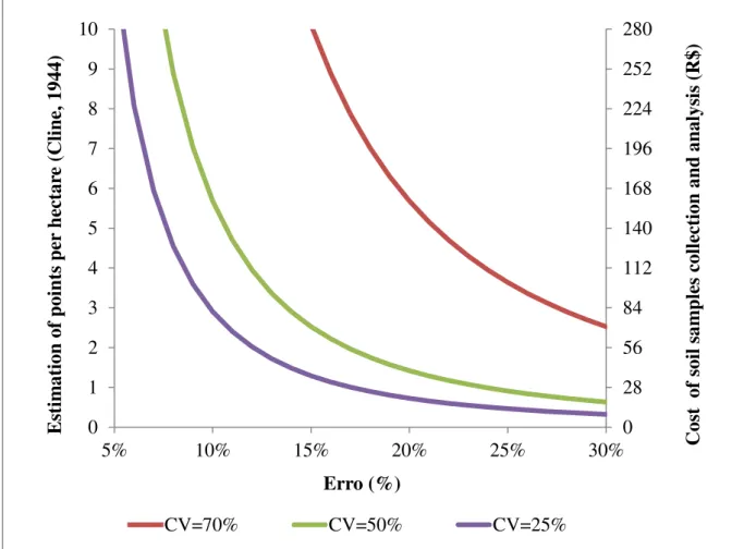
FIGURE 4. Simulation of sampling costs considering several error levels and coefficients of variation

In the studied area, the coefficient of variation of clay was 25% (blue line in Figure 4). Considering a 5% error, the number of samples required was 10 points ha−1_. This sample represents a cost of almost BRL 300.00 (considering the costs of sampling + analysis). By estimating the same coefficient of variation and increasing the error level allowed to 10%, the required number of samples to characterize the spatial variability of this attribute decreased considerably to 3 points ha−1_{, which} represents a lower cost for the producer and a lower time spent for collecting samples. When increasing the allowed error level, the amount of samples required continues to decrease. On the other hand, in the hypothetical case that the attribute under study has a higher coefficient of variation, the number of samples needed to characterize its spatial variability also increases (green and red lines in Figure 4).

The estimation presented can assist in determining the best sampling planning considering the costs and the error level to which the producer would be willing to accept. Higher error levels would be related to a lower number of samples, but it could not be enough to describe the spatial variability of soil attributes. On the other hand, in order to consider the highest number of samples for the study of variability, new technologies must be taken into account to assist in reducing sampling costs, such as the indirect quantification of soil attributes (Peluco et al. 2013; Siqueira et al., 2010a).

CONCLUSIONS

Under the studied approaches, sampling densities are different. The sampling density obtained from the geostatistics range proved to be more homogeneous. It is recommended, on average, one sample every 5.28 hectares for characterizing soil physical quality.

In the cost report, a sample density of 3 points ha−1 is suggested for elaborating variability maps with an error of up to 15% and soil attributes with a coefficient of variation close to 50%.

ACKNOWLEDGMENTS

To the National Scholarship Program abroad "Don Carlos Antonio López" (BECAL) for granting the scholarship to the first author, to the Council for the Improvement of Higher Education Personnel (CAPES) for granting scholarships (financial resources) to the other authors and to the farm Olho da Águia for providing the data set for this study.

REFERENCES

Aquino RE, Marques Júnior J, Campos MCC, Oliveira IA, Siqueira DS (2014b) Distribuição espacial de atributos químicos do solo em área de pastagem e floresta. Pesquisa Agropecuária Tropical 44(1):32-41. DOI:

https://dx.doi.org/10.1590/S1983-40632014000100001

0

28

56

84

112

140

168

196

224

252

280

0

1

2

3

4

5

6

7

8

9

10

5%

10%

15%

20%

25%

30%

Cost

of

soi

l

sam

p

les

coll

ec

tion

an

d

an

alysi

s

(R

$)

E

stim

ation

of

p

oin

ts

p

er

h

ec

tar

e

(C

li

n

e,

1944)

Erro (%)

Aquino RE, Campos MCC, Marques Júnior J, Oliveira IA, Mantovanelli BC, Soares MDR (2014c) Geoestatística na avaliação dos atributos físicos em Latossolo sob floresta nativa e pastagem na região de Manicoré, Amazonas. Revista Brasileira de Ciência do Solo 38:397-406. DOI: http://dx.doi.org/10.1590/S0100-06832014000200004 Camargo LA, Marques Júnior J, Pereira GT (2010) Spatial variability of physical attributes of an alfisol under

different hillslope curvatures. Revista Brasileira de Ciência do Solo 34(3):617-630. DOI:

http://dx.doi.org/10.1590/S0100-06832010000300003 Cambardella CA, Moorman TB, Novak JM, Karlen DL, Turco RF, Konopa AE (1994) Field-Scale Variability of Soil Properties in Central Iowa Soils. Soil Science Society American Journal 58(5):1501-1511. DOI:

http://dx.doi.org/10.2136/sssaj1994.036159950058000500 33x

Carmo DAB, Marques Júnior J, Siqueira DS, Bahia ASRS, Santos HM, Pollo GZ (2016) Cor do solo na identificação de áreas com diferentes potenciais produtivos e qualidade de café. Pesquisa Agropecuária Brasileira 51(9):161-1271. DOI:

http://dx.doi.org/10.1590/S0100-204X2016000900026

Ceddia MB, Vieira SR, Villela ALO, Mota LS, Anjos LHC, Carvalho DF (2009) Topography and spatial variability of soil physical properties. Scientia Agricola 66(3):338-352. DOI: http://dx.doi.org/10.1590/S0103-90162009000300009

Cline MG (1944) Principles of soil sampling. Soil Science 58(2):275-288.

Ding-Geng C, Peace KE (2011) Clinical trial data analysis using R. Chapman & Hall/CRC Biostatistics Series. CRC Press INC, 366p. DOI: https://dx.doi.org/10.1201/b10478 EMBRAPA – Empresa Brasileira de Pesquisa

Agropecuária (1977) Manual de métodos de análise de solo. 2ed. EMBRAPA, 212p.

EMBRAPA – Empresa Brasileira de Pesquisa

Agropecuária (2006) Sistema brasileiro de classificação de solos. 2ed. EMBRAPA, 306p.

Fortes R, Millan S, Prieto MH, Campillo C (2015) A methodology based on apparent electrical conductivity and guided soil samples to improve irrigation zoning. Precision Agriculture 16(4):441-454. DOI:

https://dx.doi.org/10.1007/s11119-015-9388-7

Grego CR, Oliveira RP, Viera SR (2014) Geoestatística aplicada a Agricultura de Precisão. In: Bernardi ACC, Naime JM, Resende AV, Basoi LH, Inamasu RY (eds). Agricultura de Precisão. Resultados de um novo olhar. EMBRAPA, p74-83.

Jenny H (1941) Factors of soil formation. A system of quantitative pedology. New York, Drover Publications. 191p.

Kerry R, Oliver MA (2004) Average variograms to guide soil sampling. International Journal of Applied Earth Observation and Geoinformation 5:307-325. DOI: https://dx.doi.org/10.1016/j.jag.2004.07.005

Kerry R, Oliver MA, Frogbrook ZL (2010) Sampling in Precision agriculture. In: Oliver MA (ed). Geostatistical Applications for Precision Agriculture. Springer, p35-63. DOI: https://doi.org/10.1007/978-90-481-9133-8_2 Marques Júnior J, Alleoni LRF, Teixeira DB, Siqueira DS, Pereira GT (2015) Sampling planning of micronutrients and aluminium of the soils of São Paulo, Brazil. Geoderma Regional 4:91-99. DOI:

http://dx.doi.org/10.1016/j.geodrs.2014.12.004

Montanari R, Pereira GT, Marques Júnior J, Souza ZM, Pazeto RJ, Camargo LA (2008) Variabilidade espacial de atributos quimicos em Latossolo e Argissolo. Ciência Rural 38(5):1266-1272. DOI:

http://dx.doi.org/10.1590/S0103-84782008000500010. Montanari R, Souza GSA, Pereira GT, Marques Júnior J, Siqueira DS, Siqueira GM (2012) The use of scaled semivariograms to plan soil sampling in sugarcane fields. Precision Agriculture 13(5):542-552. DOI:

https://dx.doi.org/10.1007/s11119-012-9265-6 Peluco RG, Marques Júnior J, Siqueira DS, Cortez LA, Pereira GT (2013) Magnetic susceptibility in the prediction of soil attributes in two sugarcane harvesting management systems. Engenharia Agrícola 33(6):1134-1143. DOI:

http://dx.doi.org/10.1590/S0100-69162013000600006

Pennock DJ, Yates TT, Braidek (2006) Towards optimum sampling for regional-scale N2O emission monitoring in Canadá. Canadian Journal of Soil Science 86(3):441-450. DOI: https://dx.doi.org/10.4141/S05-100

Oliveira IA, Campos MCC, Aquino RE, Marques Júnior J, Freitas L, Souza ZM (2014) Semivariograma escalonado no planejamento amostrall da resistencia à penetração e umidade de solo com cana-dea-acucar. Revista de Ciencias Agrárias. Amazonian Journal of Agricultural and

Environmental Science 57(3):287-296. DOI: https://dx.doi.org/10.4322/rca.ao1421

Revoredo TTO (2015) Infestação da cigarrinha das raizes (Mahanarva spp.) (Hemiptera:Cercopidae) em cana-de-açucar e planejamento amostral em diferentes formas da paisagem. Dissertação Mestrado, Universidade Estadual Paulista, Faculdade de Ciencias Agrárias e Veterinárias de Jaboticabal.

Sanchez RB, Marques Júnior J, Pereira GT, Souza ZM (2005) Variabilidade espacial de propriedades de

Latossolo e da produção de café em diferentes superficies geomorficas. Revista Brasileira de Engenharia Agricola e Ambiental 9(4):489-495. DOI:

http://dx.doi.org/10.1590/S1415-43662005000400008 Santos EOJ, Gontijo I, Silva MB, Parteli FL (2017) Sampling design of soil physical properties in a conilon coffee field. Revista Brasileira da Ciência do Solo 41:1-13. DOI: https://doi.org/10.1590/18069657rbcs20160426 SAS Institute (1995) Statistical Analysis System for Windows: Computer program manual. Cary, 705p. Silva SA, Lima JSS (2013) Atributos físicos do solo e sua relação espacial com a produtividade do café. Coffee Science 8(4):395-403. DOI:

Siqueira DS, Marques Júnior J, Matias SSR, Barron V, Torrent J, Baffa O, Oliveira LC (2010a) Correlation of properties of Brazilian Haplustalfs with magnetic susceptibility measurements. Soil Use and Management 26(4):425-431. DOI: https://dx.doi.org/10.1111/j.1475-2743.2010.00294.x

Siqueira DS, Marques Júnior J, Pereira GT (2010b) The use of landforms to predict the variability of soil and orange attributes. Geoderma 155:55-66. DOI: https://dx.doi.org/10.1016/j.geoderma.2009.11.024 Siqueira DS, Marques Júnior J, Pereira GT, Teixeira DB, Vasconcelos V, Carvalho Júnior AO, Martins ES (2015) Detailed mapping unit design based on soil–landscape relation and spatial variability of magnetic susceptibility and soil color. Catena 135:149-162. DOI:

https://dx.doi.org/10.1016/j.catena.2015.07.010 Söderström M, Soglenius G, Rodhe L, Piikki K (2016) Adaptation of regional digital soil mapping for precision agriculture. Precision Agriculture 17(5):588-607. DOI: https://dx.doi.org/10.1007/s11119-016-9439-8 Souza ZM, Marques Júnior J, Pereira GT, Montanari R (2006) Otimização amostral de atributos de latossolos considerando aspectos solo-relevo. Ciência Rural 36(3):829-836. DOI: http://dx.doi.org/10.1590/S0103-84782006000300016

Trangmar BB, Yost RS, Uehara G (1985) Application of geostatistics to spatial studies of soil properties. Advances in Agronomy 38:45-93.

Teixeira DDB, Marques Júnior J, Siqueira DS, Vasconcelos V, Carvalho OA, Martins ES, Pereira GT (2017) Sample planning for quantifying and mapping magnetic susceptibility, clay content and base saturation using auxiliary information. Geoderma 305:208-218. DOI: https://dx.doi.org/10.1016/j.geoderma.2017.06.001

Warrick AW, Nielsen DR (1980) Spatial variability of soil physical properties in the field. In: Hillel D (ed).

Applications of soil physics. New York, Academic. p319-344.

Webster R, Oliver MA (2008) Geostatistics for Environmental Scientists: Second Edition. Cornwall, Wiley. 332p.