Muhammad Hussam Khaliq
Key Features of Materials for the
Fused Deposition Modelling Process
Muhammad Hussam Khaliq
K ey F eatur es of Mater ials for t he F
used Deposition Modelling Pr
Dissertação de Mestrado
European Masters in Engineering Rheology
Trabalho efetuado sob a orientação do
Professora Doutora Olga Sousa Carneiro
Professor Doutor Luis Lima Ferrás
Muhammad Hussam Khaliq
Key Features of Materials for the
Fused Deposition Modelling Process
Acknowledgments
All praise to God Almighty, who provided me the necessary strength to accomplish this project. All respects are for the creator of this universe, whose teachings are true source of knowledge & guidance for whole mankind.
Before anybody else I thank my Parents who have always been a source of moral support, driving force behind whatever I do. I am indebted to my project advisors Prof. Olga Sousa Carneiro and Dr. Luis Lima Ferrás for their encouragements, technical discussions, inspiring guidance, remarkable suggestions, keen interest, constructive criticism and friendly discussions which enabled me to complete this project. I would also like to thanks Prof. Miguel Nobrega for his kind suggestions throughout the project. They also spared a lot of precious time in advising & helping me in writing this report.
I am also thankful to the technicians (Eng. Maurício and João Paulo) and researchers (Eng. Rui Gomes, Dr. Sacha Mould and Eng. Paulo Teixeira) of the Polymer Engineering Department, University of Minho, for their cooperation and help during different tests.
Abstract
In this work, different acrylonitrile butadiene styrene (ABS) samples (grades) are studied in order to check if the ABS used in the fused deposition modelling process has some special characteristics, or, any ABS material can be used instead. The different samples of ABS used in this study include a commercial ABS in the form of pellets used for conventional polymer processing and three ABS samples in the form of filaments that are used in different fused deposition modelling processes.
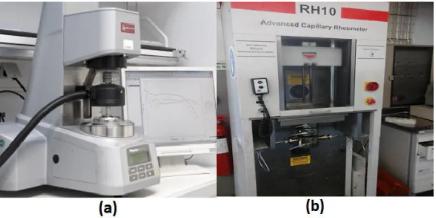
The rheological characterization of these materials is done using a stress controlled rotational rheometer (Paar Physica MCR 300) and a twin bore capillary rheometer (Rosand RH10). From the rheological characterization one could find that the pelleted ABS sample is much more viscous and elastic then the other three samples of ABS. Therefore, only two different ABS samples were used for 3D printing of pre-defined geometry specimens using the fused deposition modelling process (the pelleted ABS and one of the ABS samples in the form of filament). These 3D printed specimens were mechanically and optically analysed using the universal testing machine, INSTRON 4505, the stereoscopic magnifying glass Olympus and the digital camera Leica. This way the sintering and adhesion achieved between the extruded filaments of feedstock material for the different samples could be evaluated, and, the results obtained revealed to be in accordance with the statements made based on the rheological results.
Lastly, the numerical modelling of the flow of the polymer melt in the nozzle (liquefier) of the fused deposition modelling machine was performed, in order to check the differences between the two different materials behaviour.
It was concluded that the ABS used in fused deposition modelling process needs to have pre-defined controlled rheology.
Resumo
Neste trabalho, diferentes tipos de amostras de acrilonitrilo-butadieno-estireno (em inglês acrylonitrile butadiene styrene (ABS)) são estudados com o intuito de verificar se o ABS usado no processo de FDM (em ingês Fused Deposition
Modelling), tem ou não características especiais, ou, qualquer tipo de ABS pode ser
usado neste processo de impressão. As diferentes amostras de ABS usadas neste estudo são: o ABS comercial na fórmula de grânulos, que normalmente é usado nos processos convencionais de processamento, e, três amostras de ABS na forma de filamentos, que, são usados em diferentes processos de FDM.
A caracterização reológica destes materiais é feita usando um reómetro rotacional de tensão controlada (Paar Physica MCR 300) e ainda um reómetro capilar (Rosand RH10).
Dos resultados obtidos através da caracterização reológica foi possível concluir que o ABS na fórmula de grânulos é muito mais viscoso e elástico que as outras três amostras de ABS. Então, por forma a evitar o tratamento demasiado extensivo dos resultados, apenas duas amostras foram impressas na impressora 3D usando o método de FDM (para a impressão de objectos com geometria predefinida). As amostras escolhidas foram então o ABS na fórmula de grânulos e uma das amostras de ABS na forma de filamento.
As geometrias impressas foram submetidas a testes mecânicos e ópticos usando a máquina INSTRON 4505, usando a lupa estereoscópica da Olympus e a câmara digital Leica. Desta forma, foi possível avaliar a qualidade de sinterização e adesão entre os filamentos extrudidos, para as diferentes amostras. Os resultados obtidos revelaram estar de acordo com as conclusões tiradas através dos resultados reológicos.
Neste trabalho foi ainda feito um estudo de modelação numérica do polímero “fundido” no interior da impressora, permitindo assim fazer uma análise detalhada do escoamento nesta geometria, para as duas amostras estudadas.
Como conclusão final, podemos dizer que o ABS usado no processo de FDM necessita de uma reologia pré-definida.
Table of Contents
Acknowledgments ... iii
Abstract ... v
Resumo ... vii
List of Figures ... xi
List of Tables ... xiv
Part I Bibliographic Review ... 1
1. Introduction ... 2
1.1. Fused Deposition Modelling ... 5
1.2. Motivation/ Objectives ... 8
1.3. Route to Objectives ... 8
1.4. Thesis Structure ... 9
2. Materials and Methods ... 10
2.1. Materials ... 10
2.2. Basic Concepts: Rheology and Rheometry ... 13
2.3. Thermal Characterization/Analysis ... 17
2.4. Production of Specimens ... 20
2.4.1. Extrusion of Filament ... 20
2.4.2. 3D Printing Process ... 21
2.5. Characterization of Specimens ... 23
3. Basic concepts: Equations and Modelling ... 24
3.1. Newtonian and Generalized Newtonian Fluids ... 24
3.2. Viscoelastic Fluids ... 25
Part II Experiments, Results and Discussion ... 29
4. Experimental Results and Discussion ... 30
4.1. Rheological Testing ... 30
4.1.1. Sample 1 ... 31
4.1.2. Sample 2 ... 32
4.1.3. Sample 3 ... 34
4.1.4. Sample 4 ... 35
4.1.5. Comparison of Different Samples ... 36
4.2.1. Dimensions of the Specimens and Printing Pattern ... 38 4.2.2. Printing Conditions ... 39 4.3. Samples Performance... 42 4.3.1. Flexural Testing ... 42 4.3.2. Optical Analysis ... 45 4.4. Global Discussion ... 47
Part III Modelling ... 49
5. Numerical Modelling ... 50
5.1. Geometry, Simulation and Numerical Results ... 51
5.1.1. Viscous Results ... 52
5.1.2. Viscoelastic Results ... 54
Part IV Conclusions ... 57
Conclusions and Future Work ... 58
List of Figures
Figure 1 : Fused Deposition Modelling process, adapted from (CustomPartNet
2009) ... 3
Figure 2 : Stereo Lithography with its components, adapted from (Proto3000 2013) ... 4
Figure 3 : Selective Laser Sintering and its different parts, adapted from (Treehugger 2015) ... 5
Figure 4 : Linear Polymer with Entanglements, adapted from (W.J. Briels 1998) ... 10
Figure 5 : Cross-linked Polymer, adapted from (Donna Narsavage-Heald n.d.) ... 11
Figure 6 : Different types of Polymers, where, a small bead represents the monomer unit. Adapted from (Adhesivesandglues.com 2012) ... 11
Figure 7 : Amorphous and Crystalline structures, where small beads represent the monomer units. Adapted from (Adhesivesandglues.com 2012) ... 11
Figure 8 : Different structures of copolymers, where A and B are the different monomer units, adapted from (Fried 2014) ... 12
Figure 9 : Structural formula of ABS. Adapted from (Chemical Book 2010) ... 13
Figure 10 : Strain controlled rheometer. Adapted from (Jeffrey Gotro 2014) ... 14
Figure 11 : Stress controlled rheometer. Adapted from (Jeffrey Gotro 2014) ... 14
Figure 12 : Rotational rheometers (A) Parallel plate (B) Cone and plate (C) Concentric cylinder and (D) Torsion rectangular. Adapted from (John R. Schrei 2002) ... 15
Figure 13 : Capillary rheometer and its basic parts. Adapted from (ASI adhesives & sealants 2003) ... 15
Figure 14 : Glass transition temperature of an amorphous polymer. Adapted from (Gonzalez-Gutierrez 2015) ... 18
Figure 15 : Melting transition of crystalline polymers. Adapted from (Gonzalez-Gutierrez 2015) ... 18
Figure 16 : Differential scanning calorimetry, sample pan and reference pan. ... 19
Figure 17 : Two DSC systems (a) Heat flux DSC, (b) Power–compensation DSC, adapted from (Bhadeshia 2002) ... 19
Figure 18 : Extrusion line including auxiliary equipment’s (cooling system, puller and
cutting system), adapted from (rediff blogs 2012) ... 20
Figure 19 : FDM process and its components; (1) Feed pinch rollers, (2) Liquefier/print head and (3) Build surface ... 21
Figure 20 : Flexural testing, three point bending test. Adapted from (MatWeb 2014) ... 23
Figure 21 : Representation of the viscoelastic behaviour with a spring and dashpot26 Figure 22 : Representation of the viscoelastic behaviour with springs and dashpots (different combinations) ... 27
Figure 23 : Used rheometers (a) Paar physica (MCR 300), (b) Capillary rheometer Rosand (RH10) ... 31
Figure 24 : Sample 1, Low & High shear rate sweep, (low shear rate sweep performed with MCR 300, and high shear rate sweep is performed using RH10) .... 31
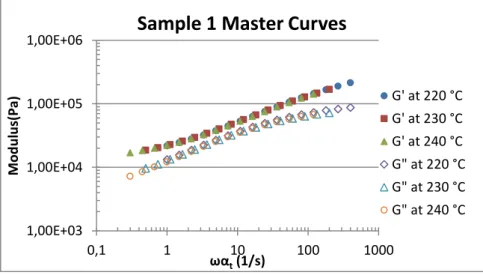
Figure 25 : Sample 1, G’ and G” master curves at 230 °C, SAOS frequency sweep .. 32
Figure 26 : Sample 2, Low & High shear rate sweep, (low shear rate sweep performed with MCR 300, and high shear rate sweep is performed using RH10) .... 33
Figure 27 : Sample 2, G’ and G” master curves at 230 °C, SAOS frequency sweep ... 33
Figure 28 : Sample 3, Low & High shear rate sweep, (low shear rate sweep performed with MCR 300, and high shear rate sweep is performed using RH10) .... 34
Figure 29 : Sample 3, G’ and G” master curves at 230 °C, SAOS frequency sweep ... 35
Figure 30 : Sample 4, shear rate sweep at 230 °C, obtained using MCR 300 ... 35
Figure 31 : Sample 4, SAOS frequency sweep, obtained using MCR 300 ... 36
Figure 32 : Viscosity (shear rate sweep) comparison, at reference temperature (230 ºC) ... 36
Figure 33 : Elastic modulus (G') comparison, at reference temperature (230 ºC) .... 37
Figure 34 : 3D printed specimen, length: 76 mm, width: 11 mm, and depth: 3.5 mm ... 38
Figure 35 : Selected 3D-Printing pattern for specimens ... 39
Figure 36 : Differential scanning calorimeter (DSC), DSC Netzsch ... 40
Figure 37 Sample 1: DSC results ... 41
Figure 40 : Sample 1, three point bending test (flexural testing). ... 43
Figure 41 : Sample 2 (50 mm/s), three point bending test (flexural testing) ... 44
Figure 42 : Sample 2 (30mm/s), three point bending test (flexural testing) ... 44
Figure 43 : Stereoscopic magnifying glass Olympus and digital camera Leica. ... 45
Figure 44 : Specimens printed using sample 1... 46
Figure 45 : Specimens printed (50 mm/s) using sample 2 ... 46
Figure 46 : Specimens printed (30 mm/s) using sample 2 ... 47
Figure 47 : Storage modulus, loss modulus and viscosity for 230 ºC (experimental data and fit obtained with the 6-mode FENE-P model for sample 2) ... 50
Figure 48 : Shear viscosity fit for sample 1 (left) and sample 2 (right). ... 51
Figure 49 : 3D printer nozzle: screw (left), schematic of the geometry where the polymer melts flows (right). ... 52
Figure 50 : Velocity magnitude for samples 1 (left) and sample 2 (right), along the channel ... 52
Figure 51 : Pressure for samples 1 (left) and sample 2 (right), along the channel .... 53
Figure 52 : Shear stress for samples 1 (left) and sample 2 (right), along the channel.54 Figure 53 : Normal stress for samples 1 (left) and sample 2 (right), along the channel. ... 54
Figure 54 : Velocity magnitude (left) and pressure (right) along the channel for sample 2 (Viscoelastic simulation). ... 55
Figure 55 : Shear (left) and normal (right) stresses along the channel for sample 2 (Viscoelastic simulation). ... 55
List of Tables
Table 1: Different rheological tests used to characterize the rheological behaviour of materials ... 17 Table 2 : Samples (grades) of acrylonitrile butadiene styrene (ABS) used in this study ... 30 Table 3 : Process parameters used in fused deposition modelling (3D printing) ... 39 Table 4 : Glass transition temperatures of ABS samples ... 40 Table 5 : Sample 1, results of three point bending test (maximum loads at breakage) ... 43 Table 6 : Sample 2 (50 mm/s), results of three point bending test (maximum loads at breakage) ... 44 Table 7 : Sample 2 (30 mm/s), results of three point bending test (maximum loads at breakage) ... 45 Table 8: Parameters used in the 6-mode FENE-P model fit... 51
Chapter 1
1. Introduction
The idea of printing goes back to the early Mesopotamian civilization before 3000 BCE, where round seals were used to print on clay tablets. Since then, printing techniques have evolved and diversified, leading, for example, to the portable ink printers that we have nowadays in our homes. Although the word “printing” is strongly associated to these ink printers, this is merely a consequence of our common sense, since “printing” embraces a broad range of techniques. Basically, different printing techniques were developed based on the personal or the group needs. For example, printing in clothes, or the mass printing of books and newspapers. With the exponential growth of technological progress and the change in people’s needs, 3D printing became a reality, allowing to print cars or even houses.
To produce a 3D object, one can use a block of material and shape it (by removing material) to a desired form or, one could try to build the desired shape by merging small portions of material. These two techniques can be catalogued as “subtractive process” and “additive process”, respectively.
Although both techniques present their own advantages, one major drawback of the subtractive process is the increase in the quantity of raw material that needs to be used for producing an object.
Additive Manufacturing (AM) or 3D printing refers to a process which uses digital design data to build up a component in layers by depositing material in several layers. It is one of the emerging technologies for the production of three dimensional objects through an additive process (Ford 2014).
The most important additive manufacturing techniques used for polymers are: (1) Fused Deposition Modelling (FDM), (2) Stereo Lithography (SLA) and (3) Selective Laser Sintering (SLS) (Puyvelde 2014). Fused Deposition Modelling will be studied in detail in this work, but firstly these three techniques are briefly explained.
In the Fused Deposition Modelling process a filament feedstock is fed into the liquefier using a pinch feed mechanism (Gibson, Rosen and Stucker 2010). This incoming solid filament acts as a plunger/ram to extrude the material through the nozzle (Reddy and Ghosh 2007). These FDM machines use, generally two kinds of materials: a modelling material which constitutes the finished object and a support material which acts as a support for the object, as illustrated in Fig. 1. In a typical FDM process, the extrusion nozzle moves over the building platform in horizontal and vertical directions, "drawing" a cross section of the final product onto the platform. Once a layer is completed, the base is lowered or the extrusion head is raised usually by about 150 micron to make room for the next layer of extruded
material. While the extruded beads/layer of material cools it binds it to the layer beneath it.
The most common material used for FDM process is acrylonitrile butadiene styrene (ABS) (Puyvelde 2014).
Figure 1 : Fused Deposition Modelling process, adapted from (CustomPartNet 2009)
There are some advantages and disadvantages when using the FDM process. One of the main advantages of the FDM process is its flexibility on the design of complex shape products, especially when soluble supports need to be used. It is a relatively simple system of 3D printing, and even desktop equipment is available for a decent price (Puyvelde 2014). The main drawback of the FDM process is the availability of a limited number of raw materials. The most used feedstock material for FDM process is ABS, which sometimes is blended with polycarbonate (PC) to improve the mechanical properties of the final product (Novakova, Ludmila and Kuric 2012). Another well-known additive process is the Stereo Lithography (SL). SL is a manufacturing process, which uses a vat of liquid ultraviolet curable photopolymer resin (like for example light-sensitive epoxy resins) with an ultraviolet laser to build the final product layer by layer. For every layer, the laser beam traces a defined cross-sectional pattern of the part on the surface of the liquid resin and the liquid resin cures and joins with the layer below, as illustrated in Fig. 2. After the pattern for one layer has been traced, the SL elevator platform descends by a distance equal to the thickness of a single layer, typically 0.05 mm to 0.15 mm, and the cross section of new layer will be traced. Once the part is build, it will be cleaned in a chemical bath to remove the excess resin, and, sometimes, is subsequently cured in an ultraviolet oven.
Figure 2 : Stereo Lithography with its components, adapted from (Proto3000 2013)
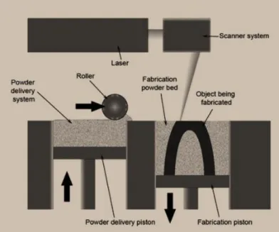
The main advantage of the Stereo Lithography is the high speed production of parts. Secondly, it is a well-known mature technology (first of the additive manufacturing methodologies). However, the major drawback for Stereo Lithography is its availability for only light-sensitive resins and the use of supports that need to be removed after production, making this technique more expensive (Puyvelde 2014). A third well-known additive method is the Selective Laser Sintering (SLS) process. In this process a laser is used to produce 3D parts that are created layer by layer in a consolidated bed of polymer, as illustrated in Fig. 3. A high power laser (for example, a carbon dioxide laser) fuses small particles of polymer to get the final three dimensional shape of the product (Hopkinson, Hague and Dickens 2006). Computer aided 3D digital description of the part is used to produce the desired cross-section on the surface of the polymer bed, and, once the cross-section in each layer is scanned, the powder bed descends a distance equal to a layer thickness being the new layer scanned on top of the previous layer until the part gets completed. The main advantage of the SLS process over other additive manufacturing processes is that it does not require any support materials because the part is produced in a compact bed of un-sintered material (Puyvelde 2014).
Figure 3 : Selective Laser Sintering and its different parts, adapted from (Treehugger 2015)
The previous text was a brief introduction on the techniques most commonly used for additive manufacturing or 3D-Printing. As mentioned earlier, fused deposition modelling is the chosen method for this work, and therefore, it will be explained in detail in the next chapters.
1.1. Fused Deposition Modelling
Rapid Prototyping is the automated production of a prototype or a final product using computer aided design. The additive manufacturing technology represents the new phase in the evolution of prototyping. The first technique for rapid prototyping become available during 1980s and it was used to produce model and prototype parts. There were more than 20 different rapid prototyping techniques by the end of 1988 being the Fused Deposition Modelling the most common method used for rapid prototyping (Chua, Leong and Lim 2003).
Some quick review on the major milestones in the history of additive manufacturing, tell us that fused deposition modelling was developed by S. Scott Crump in the late 1980s and was commercialized in 1990 by Stratasys in Eden Prairie, Minnesota (Chua, Leong and Lim 2003). In 1984 Charles Hull developed and patented Stereo Lithography. During 1986 Carl Deckard patented Selective Laser Sintering and this technology was made commercial later in 1989. In 2007 Objet Connex launched the first 3D printer that can be used to print an object with multiple materials. Urbee, which is a joint venture between Kor Ecologic and Stratasys, created the first car with a 3D printed body during 2011. During 2013 “Liberator”, the first 3D printed gun was manufactured by Defense Distributed (CEABLOG 2014).
Now, a more detailed review is presented about the fused deposition modelling process, covering the main findings from 1996 onwards.
In 1996, a group of researchers (Agarwala, et al. 1996), made improvements in the fused deposition modelling process for the production of functional ceramic and metal parts. They improved the fused deposition modelling process by eliminating several internal and surface defects that, if not eliminated, would severely limit the structural properties of the final product. They also discussed in detail the other defects present in the earlier processes and proposed several new strategies to eliminate these defects.
During 1997 Yardimci and co-workers (Yardimci, et al. 1997), proposed the complimentary computational models that can be used for the extrusion phase of fused deposition modelling. In their study, dependence of thermal behaviour on nozzle and liquefier design has been studied. Also the influence of the temperature fields near the deposition point is explained, especially for the deposition of multiple material systems.
In 2000 Thomas and Rodríguez (Thomas and Rodríguez 2000), modelled the fracture strength, which develops between the fused deposition extruded filaments, taking into account the wetting and thermally driven diffusion processes. In this work fracture toughness data of fused deposition modelled ABS is used to quantify the proposed model. The result of this study showed that fracture strength mainly develops because of slower cooling rates during solidification, which makes the bonds between the roads stronger.
During 2000, the authors (Venkataraman, et al. 2000), studied the fused deposition of ceramics (FDC). This is a production technique that uses highly filled polymers in filament form as raw material. These feedstock filaments can fail via buckling during their processing, and in this work, a methodology for finding compressive mechanical properties of filaments was developed. The authors also defined the critical limits for which the feedstock material buckles.
In 2002, Sung-Hoon Ahn and his colleagues (Ahn, et al. 2002), explained the critical material properties required for fused deposition modelling raw materials and the effect that FDM process parameters have on anisotropic material properties. The process parameters (raster orientation, air gap, bead width and modelling temperature) were examined and their effects on final product were explained. Experimental results of tensile strength and compressive strength for different ABS products obtained from different raw materials were compared, and they also built many rules for designing FDM parts based on their experimental results.
During 2003 Bellini and Güçeri (Bellini and Güçeri, Mechanical characterization of parts fabricated using fused deposition modeling 2003), concluded that broadening of material choice, improvement of the surface quality, dimensional stability and getting necessary mechanical properties for matching the performance criteria are required when shifting from prototyping to manufacturing of final product.They also
explained the mechanical characterization of products manufactured using fused deposition modelling.
In 2004 Bellehumeur and co-workers (Bellehumeur, et al. 2004), investigated the bond formation between extruded ABS filaments in the fused deposition modelling process. Thermal analysis of the fused deposition modelling process and sintering experiments were performed to explain the dynamics of bond formation between polymer filaments, and, the degree of bonding obtained during filament fused deposition was predicted quantitatively. Their main conclusion suggests that control of the cooling conditions have a strong influence on the mechanical properties of the parts fabricated using the fused deposition modelling process.
During 2004, a group of researchers (Bellini, Guceri and Bertoldi, Liquefier dynamics in fused deposition 2004), described the analysis of liquefier dynamics in order to establish strategies for controlling the flow during the extrusion phase, which is necessary to achieve the good final product in the fused deposition modelling process. They built a mathematical model based on physical assumptions in order to understand the complex phenomena that occurs inside the liquefier. They concluded that the slip between rollers and filament feedstock material are responsible for an error, when sudden changes are applied to the flow rate.
It is well-known that when there are temperature gradients in the fused deposition modelling process, thermal stresses can develop. In 2007, Wang and Jin (Wang, Xi and Jin 2007), analysed the prototype deformation during the fused deposition modelling process. Mathematical modelling of prototype warp deformation was performed, and the effect of influencing factors, such as the stacking section length, the chamber temperature, the number of deposition layers and the material linear shrinkage rate, were explained quantitatively. This work provided some methods for reducing the prototype warp deformation.
In 2008, the authors (Sun, et al. 2008), investigated the mechanism of bond formation between the filaments of extruded polymer in the fused deposition modelling process. They explained that bonding between the extruded filaments is thermally driven and determines the mechanical properties of the final product. Their experiments showed that the manufacturing strategy and the variations in the heat transfer convection coefficients affected the cooling temperature profile and, consequently, the mesostructure of the product and the bonding strength between the extruded filaments. They found that bond formation significantly depends upon the sintering phenomena, and bond formation happens for short interval of time when the temperature of filaments is above the critical sintering temperature.
During 2009 Mostafa Nikzad and his colleagues (Nikzad, et al. 2009), performed the 2D and 3D numerical modelling/analysis of the melt flow behaviour of ABS and Iron composite in the liquefier/print head of fused deposition modelling process using ANSYS FLOTRAN and CFX finite element packages. They investigated the
basic flow parameters, which include temperature, velocity and pressure drop, and they also produced ABS-iron composite filaments and checked whether they can be used for current fused deposition modelling machines. The result of their work provided good information for building melt flow models for metal plastic composites, and they also optimized FDM parameters for better quality of such composites.
In 2010 Liang and Tian (Ji and Zhou 2010), developed a 3D transient thermal finite element model for fused deposition modelling of ABS considering temperature dependent thermal conductivity and heat capacity. Their main results were that temperature field distribution is like an ellipse and the highest temperature gradient occurs near the edge of the deposited part.
During 2012 Halidi and Abdullah (Halidi and Abdullah 2012), showed that the presence of moisture affects the FDM process of ABS. Basically, they concluded that moisture affects the physical, morphological and thermal stability changes of the polymer. Also, experiments were conducted to check if these changes may have caused the blockage of the nozzle. They concluded that the blockage of the nozzle was due to the morphological and thermal stability changes of the ABS when it is exposed to moisture.
1.2. Motivation/ Objectives
- One of the motivations of this work is to study the rheological properties of acrylonitrile butadiene styrene, in order to assess the suitability of different grades (samples) of ABS to be used as feedstock material in the fused deposition modelling process.
- ABS is one of the most used feedstock materials in the fused deposition modelling process. It is used in the form of filaments and it is more expensive than the ABS available in the form of pellets. In some cases the difference is very high (of the order of 15 to 100 times higher). Therefore, the main motivation/objective of this work comes from this economic factor. Being the objective to check scientifically if there is any reason justifying this difference in prices. Also, it is intended to check if there are some major requirements/differences for the ABS grades, when they are to be used in the fused deposition modelling process.
1.3. Route to Objectives
- The first step in this work is to do the rheological characterization of different grades (samples) of ABS available in the form of pellets or filaments. The rheology of these materials is not very well characterized yet in the literature and the rheology data obtained will also be the key to detect differences between the various ABS grades (samples) used.
- The glass transition temperature of different ABS grades (samples) will be measured.
- 3D printing of different grades (samples) of ABS in predefined shape specimens.
- Lastly, these specimens will be characterized mechanically and optically. The specimens will be tested for mechanical properties via flexural testing, and, optical microscopy will be used to check the sintering and adhesion achieved for different ABS feedstock materials.
- Finally numerical and analytical modelling of the flow of the polymer in the nozzle of the fused deposition modelling machine will be performed, in order to check how different grades (samples) of ABS behave during 3D printing.
1.4. Thesis Structure
In the first chapter there is an introduction to Additive Manufacturing process, covering the state of the art on the FDM process. This chapter also explains the motivation/objectives and route towards objectives. The second chapter encompasses the theoretical description of materials and of all the different methods used in this work. The third chapter covers the basic constitutive equations used for viscous viscoelastic numerical modelling. In the fourth chapter, experimental setups and the results of rheological testing, 3D-printing using different samples of ABS and characterization of the printed specimens (mechanical and optical) is presented. This chapter also includes a detailed discussion on all the obtained results. The last chapter of the thesis is devoted to the numerical modelling of the flow of different grades of ABS in the nozzle of the fused deposition modelling machine. The thesis ends with the conclusions, and, a brief description of the proposed future work is presented.
Chapter 2
2. Materials and Methods
2.1. Materials
Polymers are made up of very large number of repeating units (monomers), and, their molecular mass varies from 10000 to 1000000 grams/mole, which is extremely high when compared to normal low molecular weight materials e.g benzene 78 g/mol and glucose 180 g/mol. The polymer molecules are in the form of long chains and those chains can be branched, linear, or even form a network (that can be temporary because of physical entanglements or permanent due to chemical crosslink between the molecules (Fried 2014)).
Polymers can be classified based on their origin: (1) natural, (2) semi synthetic and (3) synthetic. Natural polymers are abundantly present in vegetables and animal tissues e.g cellulose, wool and silk. Semi-synthetic polymers are partly from natural origin but they have been chemically modified into half synthetic polymers. Leather and technical rubber are common examples of semi-synthetic polymers. Lastly, synthetic polymers are the ones in which the network or the chains of the polymers are built from low molecular mass substances (monomers) in a chemical process. The low molecular mass components are mostly organic monomers, and, these monomers are obtained from fossil fuels. Some examples of synthetic polymers are polyethylene (PE), acrylonitrile butadiene styrene, and, polyether ether ketone (PEEK) (Fried 2014).
The other way of classifying the polymers is based on their structure. There are two main categories: (1) single chain and (2) network structure polymers. The first type, single chain polymers, as illustrated in Fig. 4, are mostly linear polymers, although these chains can be branched. The stiffness of such polymers is relatively low (Van der Vegt 2006).
In the network structure polymers, as shown in Fig. 5, molecular chains are strongly connected by primary chemical links, and flow of the network polymer is not possible as it is hindered by permanent chemical links (Van der Vegt 2006).
Figure 5 : Cross-linked Polymer, adapted from (Donna Narsavage-Heald n.d.)
Now, based on the above structural features, polymers are divided in three main categorises of practical (industrial) importance: (1) Thermoplastic (2) Thermosets and (3) Elastomers, as illustrated in Fig. 6.
Figure 6 : Different types of Polymers, where, a small bead represents the monomer unit. Adapted from (Adhesivesandglues.com 2012)
Thermoplastic: These are non-cross-linked systems, which flow at high temperatures, and, when cooled return to solid state. They can take two different forms of structures, amorphous or crystalline structures (as shown in Fig. 7) depending upon the degree of the intermolecular interactions that occur between the polymer chains (Fried 2014).
Figure 7 : Amorphous and Crystalline structures, where small beads represent the monomer units. Adapted from (Adhesivesandglues.com 2012)
Thermosets: These materials are made of polymer chains that are linked together by chemical bonds, resulting in a highly cross-linked polymer structure, as illustrated in
Fig. 6 (Fried 2014). They have high mechanical and physical strength as compared to thermoplastics or elastomers. The main limitation of thermosets is their poor
elasticity and elongation properties because of highly cross-linked structures (Van der Vegt 2006).
Elastomers: In these materials, polymer chains have slightly cross-linked (network) structure, as shown in Fig. 6. They are capable of returning to their original shapes when they are released after stretching (Van der Vegt 2006).
There are some other types of polymers, which are made up of more than one type of repeating units. They are mainly copolymers, as described below,
Copolymers: There are some properties of polymers that are obtained by linking more than one type of monomer or repeating units during polymerization (a reaction in which monomers react to form long chain polymers). When two different monomers or repeating units are polymerized to obtain desirable properties, these polymers are called copolymers (Fried 2014).
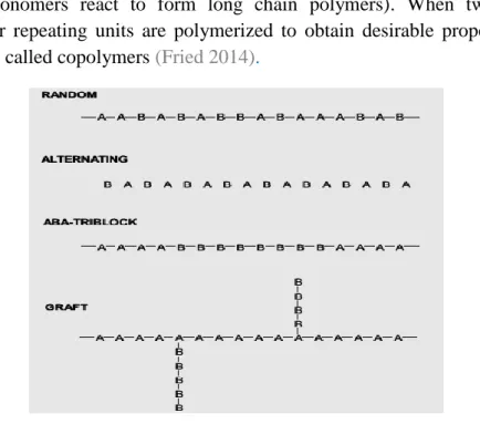
Figure 8 : Different structures of copolymers, where A and B are the different monomer units, adapted from (Fried 2014)
The linking pattern of different monomers in copolymers can be totally random or may be perfectly alternating, as illustrated in Fig. 8. Those copolymers that possess a long block of one type of monomer (A) followed by a block of another type of monomer (B) can be obtained under special reaction (polymerization). These copolymers are called block-copolymers, as shown in Fig. 8. An example of commercially important block copolymer is styrene butadiene styrene (SBS). Graft copolymerization usually results in high impact strength polymer e.g acrylonitrile butadiene styrene (ABS) (Fried 2014).
Now, a brief description of ABS will be presented, as this is the material used as feedstock in this work.
Acrylonitrile Butadiene Styrene is a thermoplastic copolymer polymer, as shown in Fig. 9, having amorphous structure. It is a terpolymer (terpolymer is a copolymer
comprised of three different monomers), which is produced by polymerizing styrene and acrylonitrile in the presence of polybutadiene. The polymerization results into a long chain of polybutadiene with shorter chains of poly (styrene-co-acrylonitrile). The main advantage of ABS is that this material combines the strength and rigidity of the acrylonitrile and styrene polymers with the toughness of the polybutadiene rubber.
Figure 9 : Structural formula of ABS. Adapted from (Chemical Book 2010)
The most important mechanical properties of ABS are toughness and impact strength, and, it is widely used in applications where impact resistance and structural strength are necessary. ABS has excellent dimensional stability. That is why it is ideal for pre-production of rapid prototypes that can accurately predict performance of final products (RedEye 2015 ).
2.2. Basic Concepts: Rheology and Rheometry
Rheology is the science of flow and deformation of matter under the effect of an applied force. The term rheology comes from the ancient Greek word rheos that means flow and logia that means the science/the study. It is normally used to describe the consistency of different material systems, with two behaviour components, viscous and elastic. Viscosity explains the resistance to flow or the friction between different layers during the flow, and, elasticity describes the stickiness or structure of the material system. The other use of rheology is that it helps us predicting the behaviour of the material in processing, and, the performance of the final product (Schowalter 1978).
In order to compare different materials, we have to define properties, such as, for example, the resistance of the material to flow. These properties can be measured with the help of rheometry.
Rheometry explains the experimental techniques that are used to determine the rheological properties of the materials to be studied. The main function of rheometry is to quantify the rheological material parameters which are practically important. The instruments that are used to measure the rheological properties of the materials are rheometers (Shenoy and Saini 1996). Their working principle is one of the following two:
1. One can apply deformation on the material and measure the force generated 2. One can apply force on the material and in response measure the deformation
There are different geometries that are used in the rheometers, and, certain calculations are performed to convert force/deformation to the corresponding stresses and strains, which then can be used to calculate material parameters (Shenoy and Saini 1996).
There are two main categories of rheometers (1) Rotational rheometers and (2) Capillary rheometers.
Rotational rheometers are used in two main modes: controlled rate and controlled stress. For the controlled rate rheometers, the material, which has to be characterized, is placed between two plates and then one of the two plates rotates at constant speed. The torsional force it produces on the other plate is measured. So, in this case, speed (strain rate) is the independent variable and torque (stress) is the dependent variable, as shown in Fig. 10, (Tabilo-Munizaga and Barbosa-Canovas 2005).
Figure 10 : Strain controlled rheometer. Adapted from (Jeffrey Gotro 2014)
For controlled stress rheometers the displacement or rotational speed (strain rate) is measured on the plate in response of a predefined torque, which is applied on the same plate, as shown in Fig. 11.
Now, let us review the different geometries that are used in rotational rheometers. Most common geometries are cone and plate, concentric cylinder, parallel plate and torsion rectangular, as shown in Fig. 12.
Figure 12 : Rotational rheometers (A) Parallel plate (B) Cone and plate (C) Concentric cylinder and (D) Torsion rectangular. Adapted from (John R. Schrei 2002)
These different geometries are used for different types of materials. Concentric cylinder geometry is used for very low to medium viscosity samples. It cannot be used for pastes because there can be air bubble formation and it will affect the results. The materials with very low to high viscosity are used in cone and plate geometry. This geometry is basically used for liquid samples it has a limitation that it can be used for dispersions; only when the particle size is less than 5 micro meter. Parallel plate geometry is used for very low viscosity liquids to soft solids. It is used for gels, pastes, soft solids and polymer melts. Torsion rectangular rheometer is used for very soft to very rigid solids (Shenoy and Saini 1996).
As mentioned earlier, the second main category of the rheometers is capillary rheometry. Its basic application is in the polymer processing industry, but it is also relevant for many other processes for example high speed coating and printing applications. These capillary rheometers (shown in Fig. 13) are based on controlled extrusion of the material through a circular die (capillary), where the material flows. Deformation properties are characterized using conditions of high force/pressure, high shear rate and high temperature.
Generally, the material is pushed from a reservoir into a capillary at constant velocity and pressure drop is measured. The measured pressure drop has entrance and exit effects. Therefore, a correction in the measured pressure drop is necessary to eliminate the entrance/exit pressure drop effects. Bagley correction is done to get the real value of pressure drop. It considers that the extra pressure drop due to end effects can be represented by an equivalent extra length of the die. So, experiments with two to four dies of same diameter, but different lengths, are performed keeping the piston speed constant. In this way end effects can be eliminated and true shear stress can be found (Shenoy and Saini 1996).
Some of the advantages of capillary rheometers are:
1. Characterization at high shear rates e.g (100 to 105 s-1);
2. It can provide an estimation of the extensional behaviour of the sample, assuming the validity of the Cogswell analysis (Padmanabhan and Christopher 1997).
3. Detection of the onset of rheological flow defects is possible. This technique also has some limitations:
1. Corrections of the data are necessary;
2. Measurement of the elastic functions is not easy;
3. Data precision is affected by viscous dissipation and flow instabilities. The previously described rotational and capillary rheometers are those applicable for shear flows, but there are some polymer processing techniques where elongational (extensional) flows are important e.g blow moulding and fiber spinning. These flows are different from shear ones, so they must be treated in a different way, to get, for example, extensional viscosity (defined as resistance to flow when the stress is applied to elongate the material). Generally, steady state extensional viscosity is very difficult to measure because both extensional rate and stress must be constant. A steady extensional rate can be obtained if the ends of the sample are pulled apart at a rate that increases exponentially with time (Shenoy and Saini 1996). The other important thing is that force should remain constant for steady state to be achieved but most of the times sample breaks before steady state can be achieved or the equipment limits exceeds (Shenoy and Saini 1996). However, several methods were attempted and are available for measuring extensional viscosity. Some of them are Meissner elongational rheometer, Sentmanat elongational rheometer and Cross-Slot elongational rheometer.
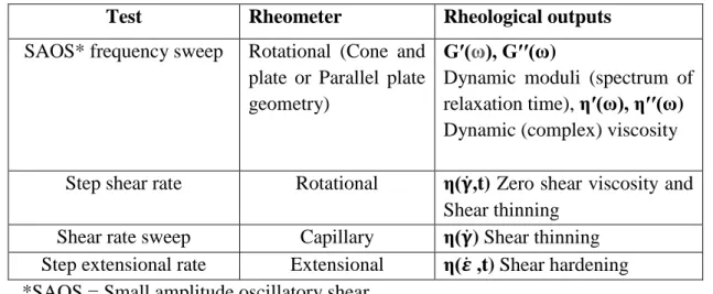
There are different rheological tests that can be performed in order to characterize different materials and these are mentioned in Table. 1.
Table 1: Different rheological tests used to characterize the rheological behaviour of materials
Test Rheometer Rheological outputs
SAOS* frequency sweep Rotational (Cone and plate or Parallel plate geometry)
Gʹ(ω), Gʹʹ(ω)
Dynamic moduli (spectrum of relaxation time), ηʹ(ω), ηʹʹ(ω) Dynamic (complex) viscosity Step shear rate Rotational η( ̇,t) Zero shear viscosity and
Shear thinning Shear rate sweep Capillary η( ̇) Shear thinning Step extensional rate Extensional η( ̇ ,t) Shear hardening *SAOS = Small amplitude oscillatory shear
2.3. Thermal Characterization/Analysis
In case of thermoplastic polymers, when thermal analysis is done, we are concerned with the two important transition temperatures:
1. Glass Transition Temperature (Tg)
2. Melting Temperature (Tm)
Glass Transition Temperature (Tg): This temperature is important in case of
amorphous polymers and for the amorphous portion of semi-crystalline polymers, but, the crystalline portion of semi-crystalline polymer remains unaffected during glass transition.
When the polymer is at low temperature its amorphous regions are in a glassy state. In this glassy state the molecules of the polymer are frozen at their positions and they possess only vibrational motions and do not have any long or short range segmental motion. In this state the polymers are hard, rigid and brittle.
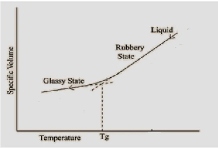
When the polymer melt is cooled from the liquid state, it becomes more viscous and flows less readily. As the temperature is reduced low enough (glass transition temperature), the polymer becomes a relatively hard and elastic material (glassy state), as illustrated in Fig. 14. When polymers are above their glass transition temperature they possess short and long range segmental motions, and they are in the rubbery state (Gonzalez-Gutierrez 2015).
Figure 14 : Glass transition temperature of an amorphous polymer. Adapted from (Gonzalez-Gutierrez 2015)
An important concept when talking about glass transition temperature, is, the free volume. As the temperature of the polymer melt is lowered, the free volume will be reduced until eventually there will not be enough free volume to allow segmental motions to take place. The temperature at which this happens corresponds to Tg, as
below this temperature the polymer is effectively frozen (Goderis 2014).
Melt Temperature (Tm): In case of semi-crystalline polymers, when they are heated
there comes a temperature at which the crystals of the polymers melt, as illustrated in
Fig. 15, and the polymer can flow easily. An important thing to be looked in the case of semi-crystalline polymers is that the degradation temperature for semi-crystalline materials is not much higher than their melting temperature.
Figure 15 : Melting transition of crystalline polymers. Adapted from (Gonzalez-Gutierrez 2015)
In order to measure and obtain these temperatures, some equipment needs to be used. In our case we have used the differential scanning calorimetry.
Differential Scanning Calorimetry (DSC): It is the most common technique used for thermal analysis (Fig. 16). Differential scanning calorimetry is used for thermal analysis/characterization of thermoplastic material. It can also be used to measure melting temperature and heat of fusion of metal alloys, to measure the glass transition temperature, melting temperature and heat capacity of the thermoplastics
The basic working principle of the DSC is based on the fact that it measures the differences in the amount of heat required to increase or decrease the temperature of sample and reference pan, as a function of temperature. The sample which is placed in the sample pan undergoes a physical transformation such as phase transitions. During this phase transition different amount of heat will flow to the sample pan as compared to the reference pan, and so, the DSC measures this different amount of heat absorbed or released during such phase transitions.
Figure 16 : Differential scanning calorimetry, sample pan and reference pan.
There are two commonly used DSC systems, (1) Heat-flux DSC and (2) Power-compensation DSC, as shown in Fig. 17. In heat-flux DSC, a low resistance heat flow path (metal disc) is used to connect the sample and the reference pan. This whole assembly is closed in a single furnace, as illustrated in Fig. 17 a. The different temperature of the sample pan relative to the reference pan is caused by enthalpy or heat capacity changes in the sample, and it results in very small heat flow (Bhadeshia 2002).
Figure 17 : Two DSC systems (a) Heat flux DSC, (b) Power–compensation DSC, adapted from (Bhadeshia 2002)
In the power-compensation DSC type two separate identical furnaces (as illustrated in Fig. 17 b) are used to control the temperatures of the sample and the reference pan. The power input of the two furnaces is varied to make the temperature of the sample and reference pan identical. The energy used to do so, quantitatively represents the enthalpy or heat capacity changes in the sample relative to the reference (Bhadeshia 2002).
2.4. Production of Specimens
2.4.1. Extrusion of Filament
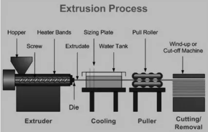
Extrusion is the most commonly and widely used polymer processing technique. A common extrusion process is illustrated in Fig. 18. There is a hopper attached to the barrel of extrusion machine which acts as the feeding point for plastic pellets or any other additives that needs to be added in order to get the final product. When material enters the extruder, it is pushed forward along the extruder barrel with the help of a rotating screw. As the polymer beads move forward along the barrel, the combination of external heating with the heating resulting from friction on the barrel walls melts the polymer beads. Once the material is completely melted, the screw further conveys the molten plastic until it exits the extruder barrel through a shaping tool (die). This shaping tool imparts a predefined shape to the molten plastic, and the extruded profile is immediately cooled down with the help of, for example, a water bath. The output of the extruder is termed as extrudate (Strong 2005).
The extrudate is pulled at a constant rate with the help of pull roller that acts as auxiliary equipment. There can also be some other auxiliary equipment for cutting the part in an exact required length, for coiling, stacking and packaging of the product for shipment.
Figure 18 : Extrusion line including auxiliary equipment’s (cooling system, puller and cutting system), adapted from (rediff blogs 2012)
It is the least expensive method to achieve high production volumes of plastic parts as it is a continuous process. Although, one of the drawbacks of the extrusion process is that it can only produce parts with constant cross section (Strong, 2005).
There are different samples (grades) of ABS that are going to be used in this work, as illustrated in Table 2 in Chapter 4. One of these samples; sample 1, is in the form of pellets. So, the extrusion process was used for producing filaments of sample 1,
because, only filaments can be used as feedstock material in fused deposition modelling.
In order to produce these filaments, the extrusion temperature was set to 190°C for the feeding section and 200 °C along the rest of the barrel. The production of the filaments was carefully controlled in order to obtain a diameter between 1.7 to 1.8 mm, as requested by the 3D printing equipment used. The rolls puller system was used to control the diameter of the filament precisely.
2.4.2. 3D Printing Process
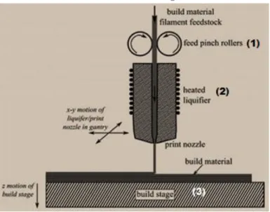
In this work, FDM is the chosen process for printing the specimens. The process was briefly explained in the introduction chapter. In this section the key features and components of the FDM process will be explained in detail. These key components include the material feeding mechanism, liquefier and print head, gantry, build surface and build environment, as illustrated in Fig. 19.
Figure 19 : FDM process and its components; (1) Feed pinch rollers, (2) Liquefier/print head and (3) Build surface
Feeding Mechanism: In conventional polymer processing techniques feedstock material is in the form of pellets but in the FDM process the typical feedstock material is in the form of filaments of varying diameters from 1.5 to 3 mm. These feedstock materials are available in different options. For the small scale systems the materials can be found in the form of loose coils while they can be found in the form of a cartridge for large scale manufacturing systems.
A pinch roll feed mechanism is used to push the filament feedstock (with the help of a motor), as illustrated in Fig. 19. The surfaces of the rolls have grooves or teeth in order to create sufficient friction between the rolls and filament to feed the liquefier at a constant rate (without slippage). Note that the compression force of the rolls leaves a minor tooth mark on the filament, but, it should be designed and controlled carefully so that it does not crush the filament (Agarwala, et al. 1996). Also, the presence of moisture in feedstock filaments can lead towards significant
problems in the FDM process as it will vaporize when it passes through the nozzle. If moisture is present in significant quantities it can cause blockage of the nozzle and the formation of bubbles in the printed samples (Halidi and Abdullah 2012). Feed stock materials available in the form of cartridge can keep the filaments dry more efficiently than simple feedstock in the form of coils.
Liquefier/print head and gantry: One of the key parts of the fused deposition modelling machine is the liquefier. It is a metal block where the filament feedstock melts, as illustrated in Fig. 19. The heating mechanism used by the liquefier to melt the feedstock is resistive heating. It is designed in such a way that it maintains uniform temperature throughout the liquefier. However, the generation of the melt in the liquefier depends on the feed rate of the material and also on the heat flux (normally the raw materials for fused deposition modelling process are amorphous polymers and they do not have defined sharp melting temperature).
The increase in temperature will lead to a decrease in the pressure drop, due to the reduction of viscosity. This reduction of viscosity will also improve the sintering and adhesion behaviour between the extruded roads or filaments.
The only drawback of using high temperature is the possibility of polymer degradation. If the polymer degrades, it can leave residue material inside the liquefier which will affect the performance of the feeding mechanism (Gibson, Rosen and Stucker 2010). Lastly, this liquefier/print head is mounted on the gantry which enables the motion of liquefier/print head in x-y plane.
Build surface: : Once the material gets melted inside the liquefier/print head then it is pushed out of the nozzle and extruded on a horizontal base surface that can move in the vertical direction (in the z-direction), as illustrated in Fig. 19. So this motion, in combination with the liquefier/print head motion (in the x-y plane), allows 3D parts to be manufactured, as shown in Fig. 19.
The temperature of the build surface is an important parameter, and, it should be controlled carefully. The temperature should be high enough so that the extruded filaments can adhere to the surface, but not so high that the part removal becomes difficult when the printing is finished.
Normally there are thermal gradients present in the printed parts as they are produced layer by layer on the build surface. If these thermal gradients are large they can distort the structure of the final product (Wang, Xi and Jin 2007).
The parts produced with the FDM process have a ridged and rough surface (inherent to the process), but this surface can be made smooth by using one of these two methods: (1) chemical smoothing and (2) mechanical smoothing (Gibson, Rosen and Stucker 2010). Also, surface coatings can be used to achieve the desired part finish.
2.5. Characterization of Specimens
Mechanical Testing: There are different mechanical properties of plastics such as the elastic modulus, Poisson’s ratio, compressive modulus and flexural modulus. These mechanical properties of the specimens can be characterized with the help of different mechanical tests. The most common type of test used to measure the mechanical properties of a material is the tensile test.
The test used in this thesis is the Flexural Test that measures the force required to bend the beam under a load which is applied at three different points, as shown in
Fig. 20. During flexural testing, the specimen (beam) is supported at two ends and the load is applied at the center of the beam by the loading nose, producing a three point bending at a defined rate.
The flexural test is used to determine the ability of the specimen to resist the deformation under bending loads, and, during the flexural test the beam is under compressive stress at the concave surface and tensile stress at the convex surface
(MatWeb 2014).
Figure 20 : Flexural testing, three point bending test. Adapted from (MatWeb 2014)
Some important parameters to be considered during flexural testing are length of the specimen, speed of the loading, and the maximum deflection. These parameters depend upon the thickness of the specimen and are defined differently by ASTM and ISO standards (MatWeb 2014).
Chapter 3
3. Basic concepts: Equations and Modelling
There are two major steps when modelling physical phenomena. The first step is to find the mathematical model that reproduces what we are trying to model, and the second step is to solve the mathematical equations.
These equations should be sophisticated enough so that they can predict well the physical phenomena ranging from small scales to big scales. The main problem is that to obtain such good models, complex mathematics needs to be used, thus making difficult the analytical solution of the models. Therefore, a numerical procedure must be adopted. We can also try to find analytical solutions for specific fluids and geometries, but in this way the model will only be adequate to describe simple systems.
In the next two subsections we present the models used to model the fluid flow in the liquefier. We will start talking about the Newtonian and inelastic non-Newtonian fluids, and then, the viscoelastic models will be discussed.
3.1. Newtonian and Generalized Newtonian Fluids
Non-Newtonian inelastic, incompressible fluids are governed by the continuity equation
. 0
u , (1)
and the momentum equation,
( ) . p . t u uu τ. (2)
In Eq. 2, u is the velocity vector, p is the pressure, τ is the deviatoric stress
tensor and the gravity contribution is incorporated in the pressure. All equations are written in a coordinate free form. The stress tensor obeys the following law for generalized Newtonian fluids,
2 ( )
τ D (3)
with the rate of strain tensor D given by,
T
1 2 D u u , (4)and ( )representing the fluid viscosity function.
For the case where viscosity is constant, ( ), we are in the presence of a Newtonian fluid. When the viscosity varies (for example, with the shear rate) it
Depending on how viscosity changes with time, the flow behaviour is characterized as thixotropic (time thinning, i.e. viscosity decreases with time) or rheopetic (time thickening, i.e. viscosity increases with time). Thixotropic fluids are quite common (e.g yogurt and paint) while rheopectic fluids (e.g gypsum paste) are very rare.
From experiments, it is well known that the viscosity of some materials depends on the shear rate. Depending on how viscosity changes with shear rate the flow behaviour is characterized as:
- Shear thinning: the viscosity decreases with increased shear rate; - Shear thickening: the viscosity increases with increased shear rate; - Plastic: exhibits a so-called yield stress value, i.e. a certain stress must be
applied before flow occurs.
Examples of shear thinning fluids are, polymer melts, paints, shampoo and ketchup. Examples of shear thickening fluids are wet sand and suspensions. Examples of plastic fluids are tooth paste and hand cream.
Based on this, several empirical models were proposed in the literature for the viscosity dependence on the second invariant of the stress tensor (which coincides with the shear rate for a simple shear deformation), and we now briefly explain some of these models.
The power law model is given by
1 ( ) a n
(5)
where a and n (n=1, Newtonian fluid; 0<n<1, shear thinning; n>1, shear thickening ) are its parameters. This model presents some limitations, such as, for example, the inexistence of a Newtonian plateau. Therefore, more sophisticated models were developed, such as the Carreau model that already accounts for these features of the Non-Newtonian fluids: 2 21 0 ( ) 1 m (6)
Here,,0,, and m are constant parameters which are determined by experimental investigations. For both models 4IID , with IID the second invariant of the rate
of strain tensor.
These models are also known as “generalized Newtonian”. Because they only describe well simple shear flows, they are not suitable for flows where the elastic effects are relevant (for example extensional flows), where new constitutive equations must be used, such as, viscoelastic models.
3.2. Viscoelastic Fluids
The key features of viscoelastic fluids, is the existence of relaxation and retardation times. When we apply a strain to a Newtonian fluid the response is
instantaneous (the relaxation time is zero or almost zero). On the other hand, if we have a viscoelastic fluid, the response will have a delay (the relaxation time is different from zero).
Maxwell proposed a viscoelastic model that couples the two components of the viscoelastic fluid behaviour (elasticity and viscosity). To represent the mechanical equivalent of this model we can assume a spring (elasticity) connected to a dashpot (viscosity), with both objects subject to the same stress, as shown in Fig. 21.
Figure 21 : Representation of the viscoelastic behaviour with a spring and dashpot
For quick deformations the fluid behaves as a Hookean elastic solid with modulus of elasticity G; for slow deformations the fluid behaves as a Newtonian fluid. For solids, the stress is given by a constant (G) times the deformation (strain)
e G
, while for a liquid, the deformation can be infinite so the measure “deformation” is of no use. Consequently, the rate of deformation (v) is used
instead, ( p v). The total rate of deformation is given by ev meaning that, 1 p d G dt (7)
With some algebra and using tensor variables, we arrive at the Maxwell model,
2 D t τ τ (8)
that can be generalized in order to become frame invariant, resulting in the Upper Convected Maxwell model,
T
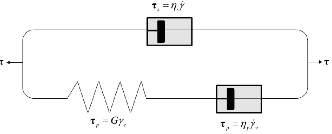
2 D with . . . t τ τ τ τ u τ u τ τ u (9)Several other models exist in the literature, and a possible way to construct new models could be the use of different combination of springs and dashpots, as shown in Fig. 22.
spring dashpot
G p
τ τ
Figure 22 : Representation of the viscoelastic behaviour with springs and dashpots (different combinations)
Not all constitutive equations are derived from combinations of spring and dashpots. Some of the models also originate from molecular or network theories.
We now present two well-known viscoelastic models, the PTT model, developed by Phan-Thien and Tanner (Phan‐Thien 1978), (Thien and Roger 1977), and the Giesekus model (Giesekus 1982).
The PTT model is described by the equation,
T
T
. . . f tr t τ τ τ u τ u τ τ u u u (10)where f tr τ
is a function depending on the trace of the stress tensor τ,D is the deformation rate tensor, is the relaxation time, is the viscosity and τstands for the Oldroyd upper convective derivative.In the literature there are two functions f tr τ
. The first one is the linearized function, given by,
1
f tr tr τ τ (11)which is acceptable for low Reynolds numbers, where small molecular deformation occurs.
The second function, is exponential and is given by,
exp
f tr tr τ τ (12)The parameter is related to the elongational behaviour that the model predicts. The Giesekus model is given by,
τ τ p Ge τ p p v τ s s τ