UNIVERSIDADE TÉCNICA DE LISBOA
INSTITUTO SUPERIOR DE ECONOMIA E GESTÃO
MASTER IN: FINANCE
VOLATILITY-SPILLOVER EFFECTS IN
EUROPEAN STOCK MARKETS
FRANCISCO MIGUEL PINHEIRO CATALÃO
Supervisor: Professor João Carlos Henrique da Costa Nicolau
Jury:
President: Professor João Luís Correia Duque Vowels: Professor José Joaquim Dias Curto
Professor João Carlos Henrique da Costa Nicolau
RESUMO
Durante as últimas décadas, temos visto como diferentes crises financeiras, que tiveram a sua origem em determinadas regiões ou países, se estenderam depois geograficamente, daí que, entender a volatilidade nos diversos mercados de acções se tenha tornado bastante importante para aqueles que têm que tomar as correctas decisões sobre a alocação de activos.
É analisada a transmissão de volatilidade dos EUA e da Europa para diversos mercados individuais de acções de vários países europeus, utilizando para esse fim um modelo GARCH de transmissão de volatilidades.
Encontrámos uma forte evidência estatística da transmissão de volatilidade dos mercados de acções dos EUA e Europa. Para os países da União Económica e Monetária os efeitos da transmissão volatilidade com origem nos EUA são mais fracos, enquanto que os efeitos da transmissão volatilidade com origem na Europa são mais fortes.
ABSTRACT
During the last decades, we have seen how different financial crisis, originated in particular regions and countries, have extended geographically, therefore, understanding volatility in stock markets has taken a very important place in determining the correct asset allocation decisions.
Volatility spillover from the US and European stock markets into individual European stock markets using a GARCH volatility-spillover model is analyzed.
We find strong statistical evidence of volatility spillover from the US and Europe stock markets. For Economic and Monetary Union countries, the US volatility-spillover effects are rather weak whereas the European volatility-spillover effects are strong.
Table of Contents
Index of Tables ... 5
Index of Figures ... 6
Acknowledgements ... 7
1.
Introduction ... 8
2.
A Brief Survey of Literature ... 12
3.
Methodology ... 22
4.
Data ... 31
5.
Results ... 39
5.1 Constant Spillover Model ... 39
5.2 Europe Spillover Model ... 47
5.3 Trend Spillover Model ... 56
6.
Conclusion ... 64
I
NDEX OFT
ABLESTable 1: Individual returns descriptive statistics ... 39
Table 2: Constant spillover model ... 40
Table 3: Variance ratios
–
constant spillover model ... 43
Table 4: Euro spillover model ... 49
Table 5: Variance ratios
–
euro spillover model ... 52
Table 6: Trend spillover model ... 57
I
NDEX OFF
IGURESFigure 1: Stock Markets Indexes ... 33
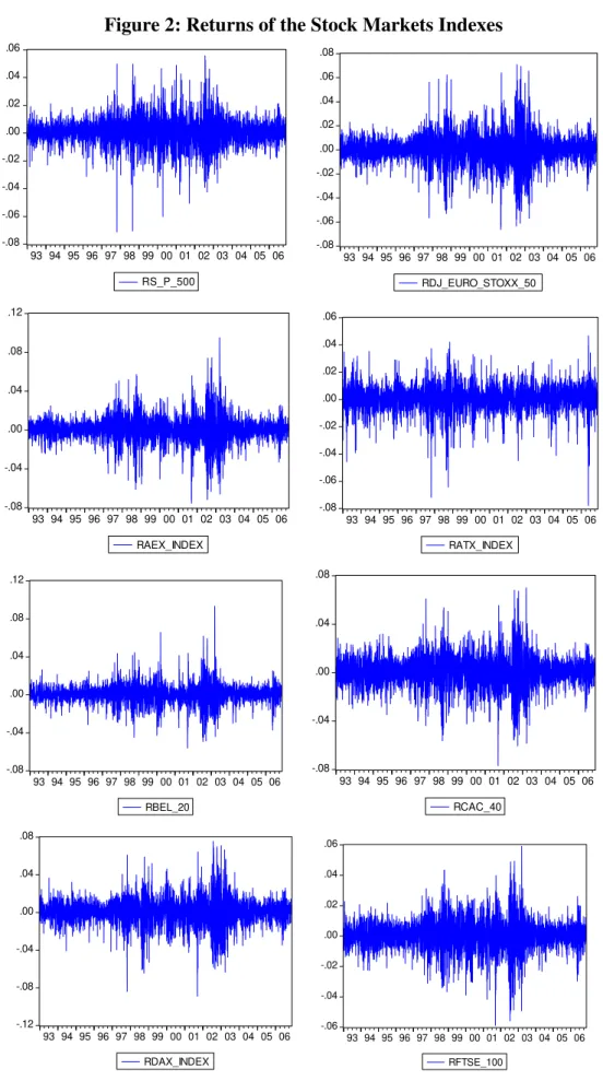
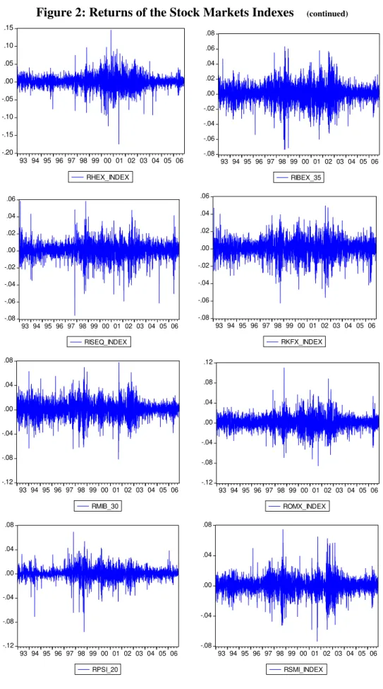
Figure 2: Returns of the Stock Markets Indexes ... 35
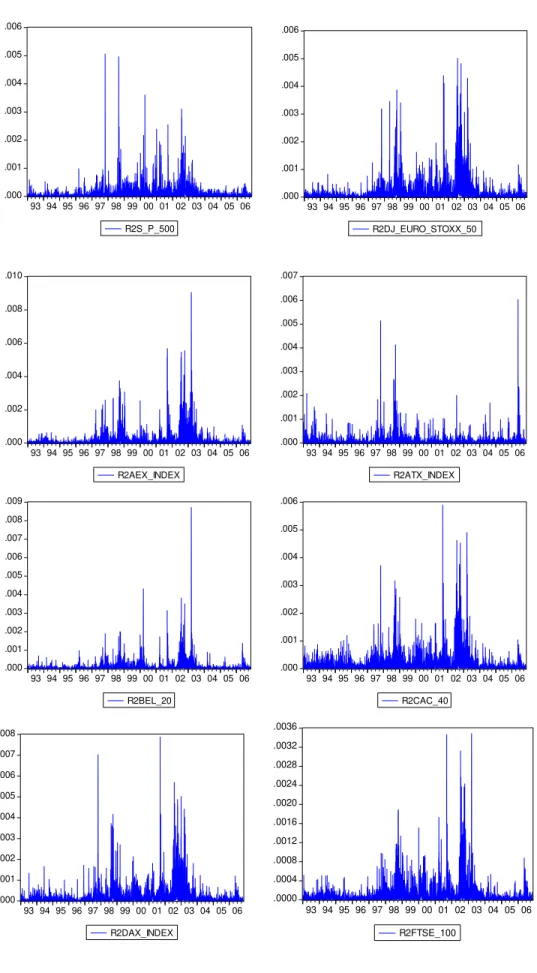
Figure 3: Squared Returns of the Stock Markets Indexes ... 37
Figure 4: Variance ratios - Germany - constant spillover model ... 44
Figure 5: Variance ratios - UK - constant spillover model ... 45
Figure 6: Variance ratios - Portugal - constant spillover model ... 45
Figure 7: Variance ratios - Spain - constant spillover model... 46
Figure 8: Variance ratios - Germany - europe spillover model ... 53
Figure 9: Variance ratios - UK - europe spillover model ... 54
Figure 9: Variance ratios - Portugal - europe spillover model... 55
Figure 10: Variance ratios - Spain - europe spillover model ... 55
Figure 1: Variance ratios - Germany - trend spillover model ... 60
Figure 2: Variance ratios - UK - trend spillover model ... 61
Figure 3: Variance ratios - Portugal - trend spillover model ... 63
A
CKNOWLEDGEMENTS1.
I
NTRODUCTIONIn the last three years, stock markets had consistent earnings, with indexes recovering from the heavy loss of the beginning of the decade. But, recently, stock markets witness a strong period of correction, the longest one in five years, with the nervousness falling again upon the investors.
This anxiety in the markets has origin in the volatility, which measures the deviation of the returns from its historical behaviour. Volatility turns the assets more risky, pulling the investor away. But, this turbulence that has rocked risky asset markets (equities, commodities, some emerging markets, and so forth) over the past months have multiple and often interlinked causes.
Uncertainty about developments in monetary policy has induced investors to remain cautious. As a result, financial markets witnessed widespread profit-taking at a time when valuations had hit their highest levels in several years. The rise in long-term interest rates since the beginning of the year, as a result of the upturn in growth, the tightening in monetary policies and the increase in inflation expectations in the wake of the reappearance of upward pressures on energy prices, has also played a role. In addition, there have been forerunning signs of a slowdown in late 2006. Lastly, the turmoil that has broken out in some major emerging countries has fuelled concern. As long as the uncertainty clouding the next monetary policy decisions to be taken by the major central banks subsists, the jitters in financial markets might persist. For, under these conditions, volatility is likely to remain
high and this will probably dampen investors’ appetite for risk, as they have been used in
United States, as well as Japan and the euro zone: unit labour costs are rising at a slow pace and the pressure exerted by factory products manufactured in low-wage countries persists. On the other hand, the financial situation of companies remains solid overall.
Furthermore, during the last decades, we have seen how different financial crisis, originated in particular regions and countries, have extended geographically. In fact, the interrelation among different countries has been a topic extensively analysed by academics and professionals for a long time. As far as international markets are becoming more and more integrated, information generated in one country can, without any doubt, affect other markets.
Before we finish this introduction, and to better understand the importance of volatility in the stock markets, we present a list of notable recessions, financial crises, depressions and downturns. All dates are approximate as the recessions began and ended in different parts of the world at different times. Also note that before detailed economic statistics began to be gathered in the nineteenth century it was very difficult to tell when recessions occurred, but prior to industrialization economic downturns usually were caused by external actions on the economic system like wars and variations of the weather.
Great Depression (1929 to late 1930s), stock market crash, banking collapse in the United States sparks a global downturn, including a second but not heavy downturn in the U.S., the Recession of 1937.
Post-Korean War Recession (1953 - 1954) - The Recession of 1953 was a demand-driven recession due to poor government policies and high interest rates.
1979 energy crisis - 1979 until 1980, the Iranian Revolution sharply increases the price of oil
Early 1980s recession - 1982 and 1983, caused by tight monetary policy in the U.S. to control inflation and sharp correction to overproduction of the previous decade which had been masked by inflation
Great Commodities Depression - 1980 to 2000, general recession in commodity prices Late 1980s recession - 1988 to 1992, collapse of junk bonds and a sharp stock crash in the United States leads to a recession in much of the West
Japanese recession - 1991 to present, collapse of a real estate bubble and more fundamental problems halts Japan's once astronomical growth
Asian financial crisis - 1997, a collapse of the Thai currency inflicts damage on many of the economies of Asia
Early 2000s recession - 2001 to 2003: the collapse of the Dot Com Bubble, September 11th attacks and accounting scandals contribute to a relatively mild contraction in the North American economy.
October 27, 1997 mini-crash: The Asian financial crisis came to a head in this crash Russian financial crisis, 1998
Dot-com bubble crash - March 2000 post-9/11 crash - September 2001
Stock market downturn of 2002 - October 2002
sell-offs, the largest drop in 10 years, triggering major drops in worldwide stock markets - February 27, 2007.
After the major Chinese market drop, the Dow Jones Industrial Average in the United States drops 416 points amid fears for growth prospects, the biggest one-day slide since the September 11, 2001 terrorist attacks. It was the 7th largest drop in the history of the Dow Jones. Sell orders are made so fast that a second analysis computer has to be used, causing an instantaneous 200-point drop at one point.
For this facts, and as long as world capital markets have become increasingly integrated, information originating from one market is likely to become more important to other markets. So, understanding the behaviour and sources of volatility is critical for pricing domestic securities, for implementing global hedging strategies and asset allocation decisions, risk sharing, economy policy and for evaluating regulatory proposals to restrict international capital flows.
In this paper we will empirically investigate the influence of the US and Europe stock markets on European individual markets returns. Specifically, we will try to estimate the magnitude of volatility-spillover effects in fourteen individual stock markets (EMU and non-EMU).
2.
A
B
RIEFS
URVEY OFL
ITERATUREOne approach widely used to quantify the magnitude of international integration has focused on estimates of volatility-spillover effects. For this purpose, ARCH/GARCH models are used by economists, which in particular, give us an estimate of a time series for the conditional variance of the relevant variables and allows for time-varying second moments.
The autoregressive conditional heteroskedastic (ARCH) model was introduced by Engle (1982) and generalized by Bollerslev (1986, 1987) and Engle, Lilien and Robins (1987), among many others.
The ARCH model, Engle (1982), was developed to capture the effect of changing volatility in a time series, where the conditional variance is a linear function of past square errors as well as possible exogenous variables.
The conditional variance at time tis a positive function of the square of last period’s
error, this in a ARCH(1), which is the simplest representation of this model.
The generalization of the ARCH model, Bollerslev (1986), was by allowing the
conditional variance to be a function not only of last period’s error squared but also of its
conditional variance. The GARCH formulation can also be extended to include squared errors from prior periods.
Engle et al (1987) introduced the ARCH-M model, which extends the ARCH model
Volatility-spillover effects are present when the unexpected shock of a given variable is driven by the innovation in a different variable. Since it is observed that time series data, and financial variables in particular, have time-varying volatility, the use of an ARCH/GARCH process to model the conditional variance turns out to be very useful. In fact, this point is crucial here, since it allows us to estimate how these effects have evolved through time.
The inclusion of the unexpected shock of a given asset return, estimated in this fashion, as the regressor of a different asset return, allows then to test for the presence of volatility-spillover effects from the first to the second asset.
This methodology has been widely employed with respect to equity markets and has generally concluded that spillover effects have increased in recent years, leading to a loss of diversification gains, in particular in periods of bear markets, which is recognized by using an asymmetric GARCH structure.
The GARCH model has been extensively applied in studies analysing relations between financial markets. This methodology allows differentiating the effects described by Engle et al. (1990) as heat waves and meteor showers. The hypothesis of heat waves is
consistent with the idea that most of the volatility sources are country specific. On the contrary, the meteor shower hypothesis is consistent with the idea of shock transmission between different markets, countries or regions.
Hamao et al. (1990) was the first study that applied the univariate GARCH
London and Tokyo and from London to Tokyo, being the related coefficients significant and positive.
Other studies that have used univariate GARCH specifications in two stages to analyse volatility transmission between financial markets are Engle et al. (1990) or Wang,
Rui and Firth (2002).
Wang et al. (2002) provides empirical evidence that Hong Kong stocks are priced to
reflect information from the London market as well as the Hong Kong market. First, the contemporaneous returns and volatility spillovers are bidirectional: there is strong evidence of returns and volatility spillovers from the SEHK (Stock Exchange of Hong Kong) to the LSE (London Stock Exchange) and from the LSE to the SEHK. However, the spillover effect from the SEHK to the LSE is stronger than that from the LSE to the SEHK.
Along literature, several types of GARCH models are used, for example a GARCH in mean model (GARCH-M) is used by Lin et al. (1994), and Hsin (2004).
Lin, Engle and Ito (1994) investigate the volatility spillover between the US and Japanese stock markets. Evidence of volatility-spillover effects is found. They used a two-stage approach that is asymptotically equivalent to a multivariate procedure if the conditional mean equations are correctly specified and if the shocks in the innovation and responding markets are mutually uncorrelated.
Hsin (2004) purposed in his article to study stock market comovements among G-7 and major Asia-Pacific developed markets in a total of 10 markets. Firstly, he used a basic aggregate shock model following the aggregate shock model proposed by Lin et al. (1994).
AR(1)-GARCH(p,q)-in-framework is also adopted by Bekaert and Harvey (1997). Lastly, an extended aggregate shock model with macroeconomic common factors is implemented. The use of the aggregate shock model proposed provide empirical results provide evidence of significant international transmission effects among these major world markets, in terms of both returns and volatility, mostly in a positive direction. The U.S. market, as expected, is the leading market in the sense that it has the most pervasive and significant impact on all markets across continents. Meanwhile, the U.S. market seems to have a different relationship with European from Asian markets. In fact, their evidence indicates that there are strong regional transmission effects.
But the most commonly used specifications in the univariate analysis of volatility transmission among markets has been the GJR - The basic model was originally proposed by Glosten, Jagannathan, and Runkle (1989) (GJR) to capture the leverage effect of volatility in stock returns - which has introduced asymmetries by means of dummy variables, see Wang et al. (2002) and Eom et al. (2002) and the EGARCH model, see Kim
(2004) and Lee et al. (2004).
timevarying influence. In general, significant dynamic information spillover effects from the U.S. were found in all the Asia-Pacific markets, but the Japanese information flows were relatively weak and the effects were country specific.
Lee et al. (2004) uses a two-stage procedure to investigate the information
transmission from the NASDAQ to the Asian second board markets. Lee et al. (2004) first
found was that, there is strong evidence of lagged returns and volatility spillovers from the NASDAQ market to the Asian second board markets when they exclude contemporaneous main board market returns. Second, there is strong evidence of contemporaneous and lagged returns and volatility spillovers from the local main board markets to the corresponding second board markets.
Edwards and Susmel (2003) suggest that an almost integrated behaviour of volatility could be due to the existence of structural changes. Edwards and Susmel (2001) also apply a bivariate SWARCH model and conclude that high volatility states tend to be related to international crisis. Their results find evidence of interdependency rather than contagion.
Bekaert and Harvey (1997), Ng (2000), Bekaert, Harvey and Ng (2005), and Baele (2005) investigate volatility-spillover effects on various equity markets using similar volatility-spillover models. They all find evidence of volatility spillover effects.
factors. In the MSCI sample, Portugal was one of eight countries with autocorrelations above 20%. Not only in Portugal was the estimation ill-behaved. Also, global optima may not have been found. Portugal, was one of two countries were the estimation of the extended model failed. The test on the variance disturbances shows evidence against the specification in only Portugal. It is possible that these residual diagnostic tests lack power.
The results suggest that only a small amount of variance is being driven by world factors. In 16 of the 19 countries, the average proportion of variance being driven by world factors is less than 10%. Portugal is one of the countries that are most affected by world factors.
The evidence also suggests that volatility decreases after liberalizations, a particularly dramatic decrease was found for Portugal.
Ng (2000) finds evidence of volatility-spillover effects to various Pacific Basin stock markets from Japan (regional effects) and the US (global effects). Baele (2005) investigates the volatility-spillover effects from the US (global effects) and aggregate European (regional effects) stock markets into various individual European stock markets. Bekaert and Harvey (1997) investigate the volatility of emerging stock markets. They distinguish between global and local shocks.
Also, Bekaert, Harvey and Ng (2005), included Portugal in their study. They find that U.S. trade impacts the conditional betas in eight of ten European countries (exceptions are Austria and Portugal), and that, Portugal was one of two countries that adhering the world CAPM at a level of 10%.
Related literature considers integration (in contrast to segmentation) of asset markets, cf. e.g. Bekaert and Harvey (1995) and Karolyi and Stulz (1996).
An important question in the two stages estimation of univariate models is to determine which and how regressors are included in the mean and variance equations to represent contagion or movement transmission between markets. Several studies use squared residuals as a proxy for the volatility of the influential market (see, for example, Hamao et al. (1990), Lin et al. (1994), Pyun et al. (2000), Wang et al. (2002) or Lee et al. (2004), among others). Other studies prefer to use the directly as a regressor estimated conditional variance series (Hamao et al. (1990) and Kim (2004)).
Finally, among the empirical literature using GARCH methodology, there exist several studies that, based on the world factor model of Bekaert and Harvey (1997), analyze the influence of global, regional and local factors on domestic volatilities (see Aggarwal et al. (1999), Ng (2000) or Hsin (2004)).
The studies about transmission of volatility effects are not only about indices and equities, take for instance the article from Eom et al.(2002) who’s study takes us to another
perspective one looks at the transmission of credit risk between two of the world’s largest
find weak volatility spillover effects, if any, from other markets to dollar swap spreads, and strong asymmetric effects of the own lagged shock in the dollar swap spreads.
Another example is the paper from Engle et al. (1990), that initiate the
volatility-spillover analysis, and that seeks to explain the causes of volatility clustering in exchange rates throw a two test hypotheses of, the already mentioned, heat waves and meteor showers. Using the GARCH model (methodology that allows to differentiate the effects described) to specify the heteroskedasticity across intra-daily market segments they find that the empirical evidence is generally against the heat wave hypothesis, or that the volatility as only country-specific autocorrelation.
Lastly, several studies highlight the relevance of the variable trade volume as explicative variable for the conditional variance, see Pyun et al. (2000) and Kim (2004). They suggest that its introduction can reduce persistency in volatility or, what is the same, that it can be an important source of conditional heteroskedasticity.
More, Wongswan (2003), analyses the effect of foreign countries macroeconomic announcements over conditional variance and trade volume. Unlike most previous studies, which only investigate information transmission through the impact on return volatility, this paper makes a first attempt to model the transmission through intraday volume. The results show strong and significant evidence of information transmission through this channel as well.
Other studies, for example, Karolyi (1995) and Booth et al. (1997), use multivariate
GARCH models.
innovations that originate in either market and that transmit to the other market depend importantly on how the cross-market dynamics in volatility are modelled.
Booth et a.l (1997) uses a multivariate EGARCH model to investigate the
asymmetric impact of good news and bad news on the volatility transmission among four Scandinavian countries.
Other studies use both univariate and multivariate ARCH models, one Engle and Susmel (1993), investigate whether international stock markets have the same volatility process, they test for a time-varying volatility process in international stock markets and the relationship between these markets within and outside each region.
With the univariate ARCH model the authors observed some similarities in the studied markets. They also observed that second moments might be related for some countries. With the multivariate ARCH the authors find two groups of countries with similar time-varying volatility.
portfolio minus the Treasury bill yield) is positively related to the predictable volatility of stock returns.
Cohen et al. (1980) follow a microstructure approach, to show that six interrelated
empirical phenomena reported in literature can be attributed to friction in the trading process causing a bid-ask-spread and price-adjustment delays that differ systematically across securities.
3.
M
ETHODOLOGYA volatility-spillover model will be applied to separate the shock to the selected European market returns in three effects:
• Local (own country)
• Regional (European Index)
• Global (USA Index)
We will use the framework proposed by Charlotte Christiansen, 2005, Volatility Spillover Effects in European Bond Markets, European Financial Management, forthcoming, which was applied successfully to European bond markets. Instead, we propose to investigate volatility spillover effects in stock markets.
This estimation process is equivalent to one used by Bekaert, Harvey and Ng (2005) which represents only practical differences to the two-step estimation procedure applied by Ng (2000) and Baele (2005).
This three-step procedure model will allow us to distinguish world from regional effects, using univariate GARCH regressions as the estimation procedures.
We will model the returns of the US and European Indices. The returns on the local markets are assumed to follow AR-GARCH processes that are extended to include volatility-spillover effects. The conditional volatility of the unexpected return is divided into the proportion caused by US, European and own country effects.
to regional effects and not in the opposite direction. The European return fails to Granger cause the US return, whereas the US return Granger causes the European return.
US Returns
The first step consists in estimating a univariate GARCH (1,1), for the US market.
The conditional return on the US index is assumed to evolve according an AR(1) process,
, 0, 1, , 1 ,
US t US US US t US t
R c c R e (1)
where, 2
, | 1~ (0, ,)
US t t US t
e I N the idiosyncratic shock, is normally distributed with mean 0
and the conditional variance follows the GARCH (1,1) specification.
2 2 2 2
, 1 , , 1 , 1
( us t| t ) US t US US US t US US t
E e I e (2)
Where US 0 and US, US 0 to make sure the variance is positive, and 1
US US and c1,US 1to ensure stationarity.
Equation (1) defines the mean-return of the US market as a simple auto-regressive process of order one.
European Returns
We follow the assumption that the shocks on the return of the European market is
driven by the idiosyncratic shock of the US market’s return. The difference for the US
Index in the mean-return equation, and from the assumption that the shock on the return of the European market is driven by the idiosyncratic shock of the US market’s return.
Hence, the European market is described by the following three equations, where
,
E t represents the total unexpected shock on the return, and eE t, the idiosyncratic shock,
therefore, the return on the European Index is assumed to be described by the following extended AR (1) specification:
, 0, 1, , 1 1 , 1 , 1 , ,
E t E E E t t US t E t US t E t
R c c R R e e (3)
, , 1 , ,
E t E t eUS t eE t (4)
where, just like before, 2
, | 1 ~ (0, ,)
E t t E t
e I N the idiosyncratic shock, is normally distributed
with mean 0 and the conditional variance follows the GARCH (1,1) specification.
The conditional mean of the European return depends on its own lagged return as well as the lagged US return. The mean spillover effects are introduced by the lagged US return, RUS t, 1. The volatility spillover from the US to Europe takes place via the
penultimate term, eUS t, . Thus, the European return depends on the US idiosyncratic shock.
In the practical estimation, the residual from equation (1) is used in place of eUS t, .
The idiosyncratic shock, eE t, , has mean 0 and conditional variance:
2 2 2 2
, 1 , , 1 , 1
( E t | t ) E t E E E t E E t
Country i Returns
The last step consists of providing a model for the individual country returns. The mean specification for the European return in equation (3) is extended even further.
, 0, 1, , 1 1 , 1 , 1 , 1 , 1 , , 1 , ,
i t i i i t i t US t i t E t i t US t i t E t i t
R c c R R R e e e (6)
Again, 2
, | 1~ (0, ,)
i t t i t
e I N the idiosyncratic shock, is normally distributed with
mean 0 and the conditional variance follows the GARCH (1,1) specification.
The conditional country i mean return depends on the lagged US, European and
own return. This specification allows mean spillover effects from both the US and European returns to the individual countries by the lagged returns RUS t, 1 and RE t, 1.
Volatility spillover effects from the US and Europe to the individual countries are introduced by the idiosyncratic US and Europe shocks, eUS t, and eE t, .
In the estimation, the residuals from equation (1) and (3) are applied as explanatory variables.
The idiosyncratic country shocks have the same distributional assumptions as the one before, therefore ei t, has mean 0 and conditional volatilities follow the GARCH (1,1) specification:
2 2 2 2
, 1 , , 1 , 1
( i t| t ) i t i i i t i i t
Notice that the non-negative and stationarity conditions that were required for coefficients of equation (2), should apply to the coefficients of equations (5) e (7).
Variance Ratios
We assume the idiosyncratic shocks eUS t, , eE t, and ei t, (for i= 1,…,N) to be
independent. However, this will not be applied to the unexpected returns:
, ,
US t eUS t (8)
, , 1 , ,
E t E t eUS t eE t (9)
, , 1 , , 1 , ,
i t i t eUS t i t eE t ei t (10)
Following this identity we are assuming, from (8) that for the US no other market has any influence on their market1.
It follows from (10) that the conditional variance of the unexpected return of country i based on the information available at time t 1 (It 1)is given by:
2 2 2 2 2 2
, 1 , 1 , , 1 , ,
( i t | t ) it i t US t i t E t i t
E I h (11)
The conditional variance of the unexpected return for country i depends on the
variance of the US, European, and own idiosyncratic shocks.
When for example the US idiosyncratic volatility is large, the volatility of the unexpected returns for country i also tends to be large if i t, 1 is significant.
This is what is denoted by volatility spillover effects.
So the significance of the parameters i t, 1 and i t, 1 determine whether volatility
spillover effects from the US and Europe, respectively, are presented in country i.
The conditional variance of the European unexpected return depends only on the US and its own idiosyncratic volatility, as shown in equation (9). So, there is volatility spillover from the US to the aggregate European stock market. The conditional variance of the US unexpected return is equal to the variance of the US idiosyncratic shock, also seen in equation (8).
Equation (11) also show us that the return volatility of market i is positively related
to the conditional variances of the US and European market. Under this specification, we can investigate whether potential asymmetric effect in the US and /or regional markets induce asymmetry in the conditional return volatility of any equity market.
We measure the proportion of the variance of the unexpected return of country i,
that is caused by the US and European volatility spillover effects, respectively, as given by equation (11). To this end, we define the following variance ratios:
2 2
, 1 , ,
,
i t US t US
i t
i t
VR
Equation (12) gives us the proportion of the total of the unexpected return that is directly explained by the variance of the US market.
2 2
, 1 , ,
,
i t E t E
i t
i t
VR
h (13)
Equation (13) gives us the proportion justified by the European market’s volatility.
The variance ratios take on values between 0 and 1.
The remaining part of the variance of the unexpected return for country i is caused
by pure local effects;
2 ,
, 1 , ,
i t
i US E
i t i t i t
it
VR VR VR
h (14)
The above equation retrieves the weight of the local shock.
The variance ratios provide a measure of the impact of global, regional, and local effects on the local variance.
We find evidence in favour of presence of volatility spillover effects when the coefficients E t, 1, i t, 1 and i t, 1 are statistically significant.
First, the spillover parameters are assumed to be constant throughout the entire sample period; the constant spillover model:
,
i t i t
,
i t i t
,
i t i t
,
i t i t (15)
Second, the spillover parameters are assumed to be constant before and after the introduction of the euro; the euro spillover model:
, 0, 1,
i t i iDt
, 0, 1,
i t i iDt
, 0, 1,
i t i iDt
, 0, 1,
i t i iDt (16)
Third, the spillover parameters undergo a gradual transition by taking on a different value each year in the sample, the trend spillover model:
, 0, 1,
i t i iDTt
, 0, 1,
i t i iDTt
, 0, 1,
i t i iDTt
, 0, 1,
i t i iDTt (17)
4.
D
ATAOn January 1, 1999, starts stage three of the EMU the euro becomes the single currency of the member states of the EMU, with the irrevocability of the conversion rates between the different former national currencies of the participating member states and the euro. From that day, the responsibility for the definition and execution of the monetary policies was delivered to the European System of Central Banks. A single monetary policy started to be conducted in euros, and the monetary markets of all the member states started to work in euros. Public Debt in the member states started to be issued in the new currency. All financial operations processed throw the banking system, which do not involved coins and motes, could be done either in national currency or in euros. This situation last for three years.
On January 1, 2002, starts the euro cash changeover with the introduction of euro banknotes and coins. The new currency becomes the sole legal tender in the euro area by the end of February 2002.
In their study of emerging markets, which included Portugal, the data used by Bekaert and Harvey (1997), ends on December 1992.
Furthermore, Bekaert, Harvey and Ng (2005), whose paper includes in their analyses the Portuguese and Spanish cases the data period ranges from January 1980/January 1986 to December 1998.
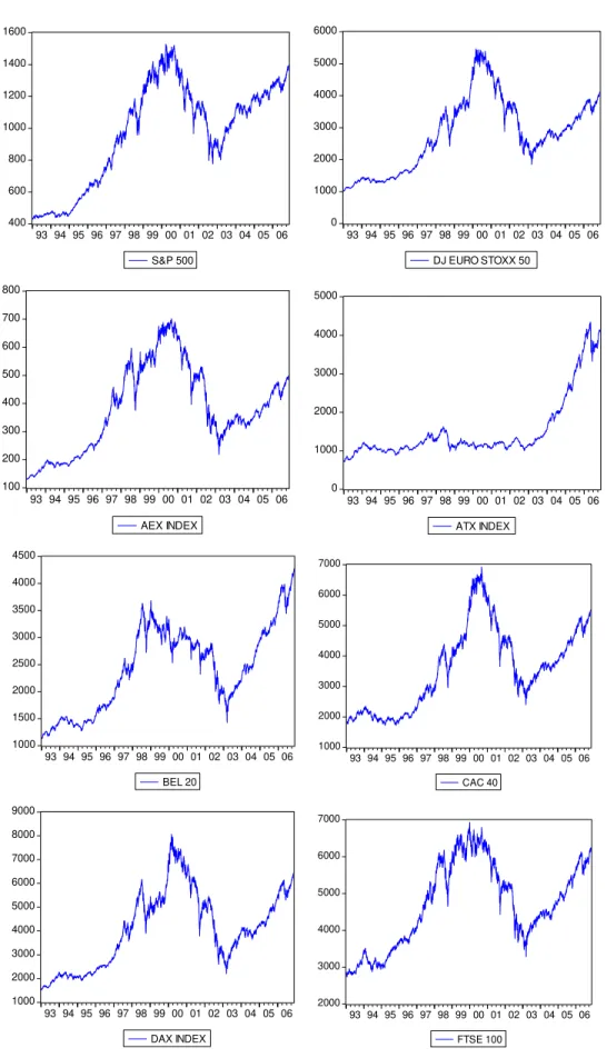
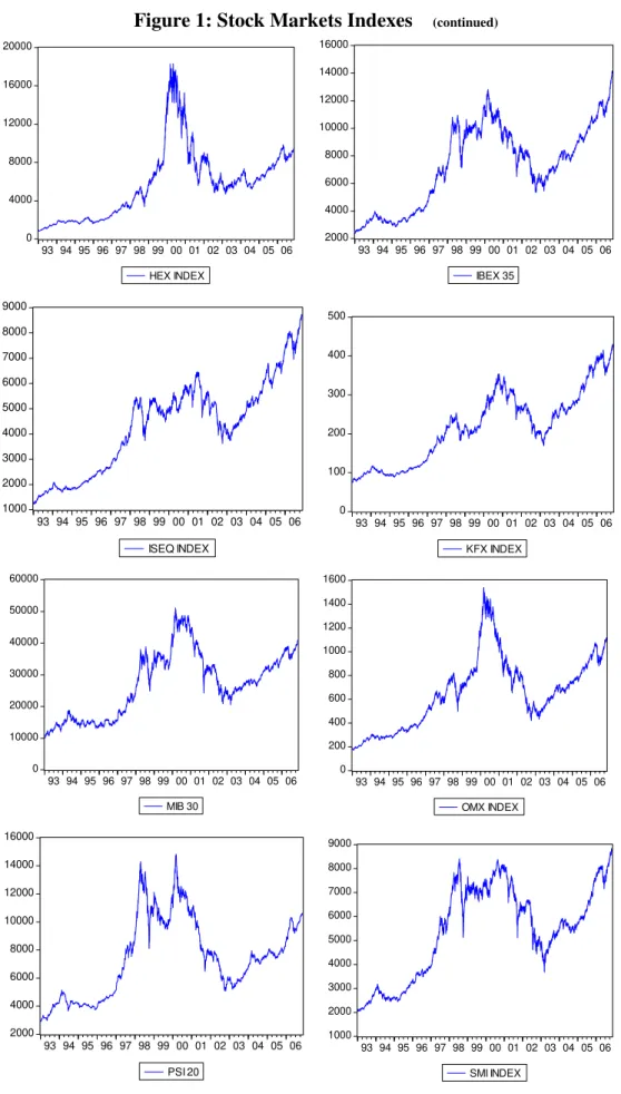
We use financial time series of fourteen European Index, for which corresponds the same number of countries, namely Austria - ATX Index, Belgium - BEL 20, Denmark - KFX Index (OMX Copenhagen 20), England - FTSE 100, Finland - HEX Index (OMX Helsinki 25), France - CAC 40, Germany - DAX Index, Ireland - ISEQ Index, Italy - MIB 30, Netherlands - AEX Index, Portugal - PSI 20, Spain - IBEX 35, Sweden - OMX Index (OMX Stockholm 30), Swiss - SMI Index.
For the US market effect, we use the S&P 500, which is an index containing the stocks of 500 Large-Cap corporations, most of which are American. All of the stocks in the index are those of large publicly held companies and trade on the two largest US stock markets, the New York Stock Exchange and Nasdaq. The S&P 500 is one of the most widely watched index of large-cap US stocks. It is considered to be a bellwether for the US economy and is a component of the Index of Leading Indicators The index is the most notable of the many indices owned and maintained by Standard & Poor's.
For the regional market effect and as a European Index we will use the Dow Jones Euro STOXX 50 Index, which is a capitalization-weighted index of 50 European blue-chips stocks from those countries participating in the EMU. It has the stated objective to provide a blue-chip representation of Supersector leaders in the Eurozone. Covers Austria, Belgium, Finland, France, Germany, Greece, Ireland, Italy, Luxembourg, the Netherlands, Portugal and Spain. As a unique aspect, we can state that this index captures approximately 60% of the free float market capitalisation of the Dow Jones EURO STOXX Total Market Index, which in turn covers approximately 95% of the free float market capitalisation of the represented countries.
Figure 1: Stock Markets Indexes 400 600 800 1000 1200 1400 1600
93 94 95 96 97 98 99 00 01 02 03 04 05 06
S&P 500 0 1000 2000 3000 4000 5000 6000
93 94 95 96 97 98 99 00 01 02 03 04 05 06
DJ EURO STOXX 50
100 200 300 400 500 600 700 800
93 94 95 96 97 98 99 00 01 02 03 04 05 06
AEX INDEX 0 1000 2000 3000 4000 5000
93 94 95 96 97 98 99 00 01 02 03 04 05 06
ATX INDEX 1000 1500 2000 2500 3000 3500 4000 4500
93 94 95 96 97 98 99 00 01 02 03 04 05 06
BEL 20 1000 2000 3000 4000 5000 6000 7000
93 94 95 96 97 98 99 00 01 02 03 04 05 06
CAC 40 1000 2000 3000 4000 5000 6000 7000 8000 9000
93 94 95 96 97 98 99 00 01 02 03 04 05 06
DAX INDEX 2000 3000 4000 5000 6000 7000
93 94 95 96 97 98 99 00 01 02 03 04 05 06
Figure 1: Stock Markets Indexes (continued) 0 4000 8000 12000 16000 20000
93 94 95 96 97 98 99 00 01 02 03 04 05 06
HEX INDEX 2000 4000 6000 8000 10000 12000 14000 16000
93 94 95 96 97 98 99 00 01 02 03 04 05 06
IBEX 35 1000 2000 3000 4000 5000 6000 7000 8000 9000
93 94 95 96 97 98 99 00 01 02 03 04 05 06
ISEQ INDEX 0 100 200 300 400 500
93 94 95 96 97 98 99 00 01 02 03 04 05 06
KFX INDEX 0 10000 20000 30000 40000 50000 60000
93 94 95 96 97 98 99 00 01 02 03 04 05 06
MIB 30 0 200 400 600 800 1000 1200 1400 1600
93 94 95 96 97 98 99 00 01 02 03 04 05 06
Figure 2: Returns of the Stock Markets Indexes -.08 -.06 -.04 -.02 .00 .02 .04 .06
93 94 95 96 97 98 99 00 01 02 03 04 05 06
RS_P_500 -.08 -.06 -.04 -.02 .00 .02 .04 .06 .08
93 94 95 96 97 98 99 00 01 02 03 04 05 06
RDJ_EURO_STOXX_50 -.08 -.04 .00 .04 .08 .12
93 94 95 96 97 98 99 00 01 02 03 04 05 06
RAEX_INDEX -.08 -.06 -.04 -.02 .00 .02 .04 .06
93 94 95 96 97 98 99 00 01 02 03 04 05 06
RATX_INDEX -.08 -.04 .00 .04 .08 .12
93 94 95 96 97 98 99 00 01 02 03 04 05 06
RBEL_20 -.08 -.04 .00 .04 .08
93 94 95 96 97 98 99 00 01 02 03 04 05 06
RCAC_40 -.12 -.08 -.04 .00 .04 .08
93 94 95 96 97 98 99 00 01 02 03 04 05 06
RDAX_INDEX -.06 -.04 -.02 .00 .02 .04 .06
93 94 95 96 97 98 99 00 01 02 03 04 05 06
Figure 2: Returns of the Stock Markets Indexes (continued) -.20 -.15 -.10 -.05 .00 .05 .10 .15
93 94 95 96 97 98 99 00 01 02 03 04 05 06
RHEX_INDEX -.08 -.06 -.04 -.02 .00 .02 .04 .06 .08
93 94 95 96 97 98 99 00 01 02 03 04 05 06
RIBEX_35 -.08 -.06 -.04 -.02 .00 .02 .04 .06
93 94 95 96 97 98 99 00 01 02 03 04 05 06
RISEQ_INDEX -.08 -.06 -.04 -.02 .00 .02 .04 .06
93 94 95 96 97 98 99 00 01 02 03 04 05 06
RKFX_INDEX -.12 -.08 -.04 .00 .04 .08
93 94 95 96 97 98 99 00 01 02 03 04 05 06
RMIB_30 -.12 -.08 -.04 .00 .04 .08 .12
93 94 95 96 97 98 99 00 01 02 03 04 05 06
ROMX_INDEX -.12 -.08 -.04 .00 .04 .08
93 94 95 96 97 98 99 00 01 02 03 04 05 06 -.08 -.04 .00 .04 .08
Figure 3: Squared Returns of the Stock Markets Indexes .000 .001 .002 .003 .004 .005 .006
93 94 95 96 97 98 99 00 01 02 03 04 05 06
R2S_P_500 .000 .001 .002 .003 .004 .005 .006
93 94 95 96 97 98 99 00 01 02 03 04 05 06
R2DJ_EURO_STOXX_50 .000 .002 .004 .006 .008 .010
93 94 95 96 97 98 99 00 01 02 03 04 05 06
R2AEX_INDEX .000 .001 .002 .003 .004 .005 .006 .007
93 94 95 96 97 98 99 00 01 02 03 04 05 06
R2ATX_INDEX .000 .001 .002 .003 .004 .005 .006 .007 .008 .009
93 94 95 96 97 98 99 00 01 02 03 04 05 06
R2BEL_20 .000 .001 .002 .003 .004 .005 .006
93 94 95 96 97 98 99 00 01 02 03 04 05 06
R2CAC_40 .000 .001 .002 .003 .004 .005 .006 .007 .008
93 94 95 96 97 98 99 00 01 02 03 04 05 06
R2DAX_INDEX .0000 .0004 .0008 .0012 .0016 .0020 .0024 .0028 .0032 .0036
93 94 95 96 97 98 99 00 01 02 03 04 05 06
R2FTSE_100
Figure 3: Squared Returns of the Stock Markets Indexes (continued) .000 .004 .008 .012 .016 .020 .024 .028 .032
93 94 95 96 97 98 99 00 01 02 03 04 05 06
R2HEX_INDEX .000 .001 .002 .003 .004 .005 .006
93 94 95 96 97 98 99 00 01 02 03 04 05 06
R2IBEX_35 .000 .001 .002 .003 .004 .005 .006
93 94 95 96 97 98 99 00 01 02 03 04 05 06
R2ISEQ_INDEX .000 .001 .002 .003 .004
93 94 95 96 97 98 99 00 01 02 03 04 05 06
R2KFX_INDEX .000 .001 .002 .003 .004 .005 .006 .007
93 94 95 96 97 98 99 00 01 02 03 04 05 06
R2MIB_30 .000 .002 .004 .006 .008 .010 .012 .014
93 94 95 96 97 98 99 00 01 02 03 04 05 06
R2OMX_INDEX .000 .002 .004 .006 .008 .010
93 94 95 96 97 98 99 00 01 02 03 04 05 06 .000 .001 .002 .003 .004 .005 .006
5.
R
ESULTSWe estimate the model using the E-views ARCH – Autoregressive Conditional Heteroskedasticity method with heteroskedasticity consistent covariance (Bollerslev-Wolldridge) option.
But before, we have estimated our model without the ARCH effect in order to realize a Lagrange multiplier test, an ARCH-LM test.
The results indicate the presence of heteroskedasticity, in other words there is a strong evidence of the presence of ARCH effect, what justify the model through the use of ARCH effects.
Constant Spillover Model
Table 2 reports the results from estimating the constant spillover model. The US results are shown in the first row of Table 2. The AR(1) parameter ^
1,US
c (0.002772) is
small, positive, and insignificant, which implies no (or weak negative) first-order autocorrelation, consistent with the summary statistics reported in Table 1.
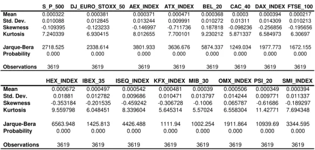
Table 1: Individual returns descriptive statistics
S_P_500 DJ_EURO_STOXX_50 AEX_INDEX ATX_INDEX BEL_20 CAC_40 DAX_INDEX FTSE_100
Mean 0.000322 0.000381 0.000371 0.000471 0.000368 0.0003 0.000394 0.000217
Std. Dev. 0.010088 0.012845 0.013244 0.009991 0.010272 0.01311 0.014309 0.010213
Skewness -0.109395 -0.123233 -0.146997 -0.711736 0.187818 -0.098236 -0.256856 -0.195656
Kurtosis 7.240339 6.930415 8.012655 7.700101 9.230212 5.871337 6.584973 6.30697
Jarque-Bera 2718.525 2338.614 3801.933 3636.676 5874.337 1249.034 1977.773 1672.155
Probability 0.000 0.000 0.000 0.000 0.000 0.000 0.000 0.000
Observations 3619 3619 3619 3619 3619 3619 3619 3619
HEX_INDEX IBEX_35 ISEQ_INDEX KFX_INDEX MIB_30 OMX_INDEX PSI_20 SMI_INDEX Mean 0.000672 0.000497 0.000542 0.000481 0.00039 0.000506 0.000349 0.000394
Std. Dev. 0.01881 0.012782 0.009686 0.010471 0.013797 0.014244 0.009771 0.011337
Skewness -0.353184 -0.201535 -0.459242 -0.306728 -0.1006 0.065787 -0.61686 -0.189297
Kurtosis 9.559798 6.048451 8.339604 5.645314 5.57024 6.558304 11.42771 7.694348
Jarque-Bera 6563.948 1425.813 4426.488 1111.94 1002.254 1911.864 10939.69 3344.595
Probability 0.000 0.000 0.000 0.000 0.000 0.000 0.000 0.000
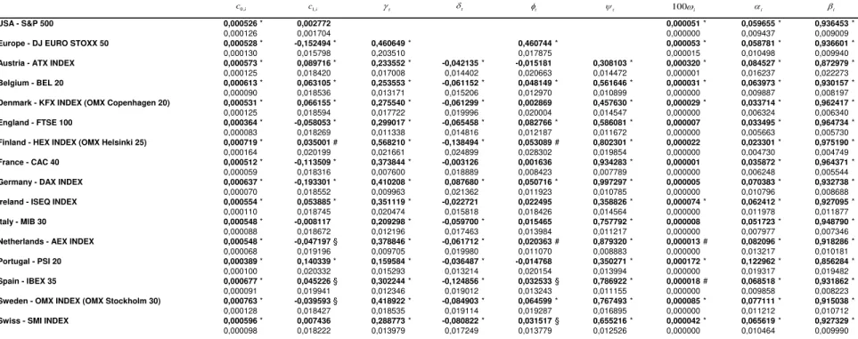
Table 2: Constant spillover model
The table reports the results from estimating the constant spillover model. Estimated parameters and standard errors below - *, §, #, indicates that the value is significant at a 1%, 5% or 10% level of significance, respectively.
USA - S&P 500 0,000526* 0,002772 0,000051* 0,059655* 0,936453*
0,000126 0,001704 0,000000 0,009437 0,009009
Europe - DJ EURO STOXX 50 0,000528* -0,152494* 0,460649* 0,460744* 0,000053* 0,058781* 0,936601*
0,000130 0,015798 0,203510 0,017875 0,000015 0,010498 0,009940
Austria - ATX INDEX 0,000573* 0,089716* 0,233552* -0,042135* -0,015181 0,308103* 0,000320* 0,084527* 0,872979*
0,000125 0,018420 0,017008 0,014402 0,020663 0,014472 0,000001 0,016237 0,022273
Belgium - BEL 20 0,000613* 0,063105* 0,253553* -0,061152* 0,048149* 0,561646* 0,000031* 0,063973* 0,930157*
0,000090 0,018536 0,013171 0,015206 0,012970 0,010899 0,000000 0,009887 0,008197
Denmark - KFX INDEX (OMX Copenhagen 20) 0,000531* 0,066155* 0,275540* -0,061299* 0,002869 0,457630* 0,000029* 0,033714* 0,962417*
0,000125 0,018594 0,017722 0,019996 0,020004 0,014547 0,000000 0,006324 0,006340
England - FTSE 100 0,000364* -0,058053* 0,299017* -0,065458* 0,082766* 0,586081* 0,000007 0,033495* 0,964734*
0,000083 0,018269 0,011338 0,014816 0,012187 0,011672 0,000000 0,005663 0,005730
Finland - HEX INDEX (OMX Helsinki 25) 0,000719* 0,035001# 0,568210* -0,138494* 0,053089# 0,802301* 0,000022 0,023301* 0,975190*
0,000164 0,020199 0,021661 0,024899 0,028302 0,019854 0,000000 0,004730 0,004749
France - CAC 40 0,000512* -0,113509* 0,373844* -0,003126 0,001636 0,934283* 0,000001 0,035872* 0,964371*
0,000059 0,018316 0,007600 0,018889 0,008423 0,007789 0,000000 0,006248 0,005544
Germany - DAX INDEX 0,000637* -0,193301* 0,410208* 0,087680* 0,050716* 0,997297* 0,000005 0,070383* 0,932738*
0,000070 0,018552 0,009963 0,021362 0,011923 0,010785 0,000000 0,010796 0,008688
Ireland - ISEQ INDEX 0,000554* 0,053885* 0,351119* -0,022721 0,022495 0,358826* 0,000074* 0,062412* 0,927095*
0,000110 0,018745 0,020474 0,015818 0,018426 0,014564 0,000000 0,011978 0,011877
Italy - MIB 30 0,000548* -0,008117 0,209298* -0,059700* 0,015465 0,757792* 0,000008 0,051723* 0,948790*
0,000088 0,018672 0,012196 0,017463 0,013984 0,011217 0,000000 0,007977 0,007346
Netherlands - AEX INDEX 0,000548* -0,047197§ 0,378846* -0,061712* 0,020363# 0,879320* 0,000013# 0,082096* 0,918286*
0,000068 0,019196 0,009705 0,019980 0,011070 0,008883 0,000000 0,013217 0,010181
Portugal - PSI 20 0,000389* 0,140339* 0,159584* -0,036487* -0,014768 0,350271* 0,000172* 0,122962* 0,856284*
0,000100 0,020332 0,015293 0,013214 0,020154 0,013994 0,000000 0,019317 0,019482
Spain - IBEX 35 0,000677* 0,045226§ 0,302244* -0,124856* 0,032533§ 0,786922* 0,000018# 0,068518* 0,931862*
0,000091 0,019941 0,012346 0,019012 0,013243 0,011155 0,000000 0,009858 0,008223
Sweden - OMX INDEX (OMX Stockholm 30) 0,000763* -0,039593§ 0,418922* -0,084903* 0,064599* 0,767493* 0,000085* 0,077111* 0,915038*
0,000128 0,018427 0,018535 0,019114 0,019287 0,016895 0,000000 0,011212 0,010712
Swiss - SMI INDEX 0,000596* 0,007436 0,288773* -0,080822* 0,031517§ 0,655216* 0,000042* 0,065619* 0,927329*
0,000098 0,018222 0,013979 0,017249 0,013779 0,012526 0,000000 0,010464 0,009990
t t t t 100 i i i
0,i
The volatility process is highly persistent in that ^ ^
US US equals 0.996. The second row of Table 2 reports the results for the European index. Own lagged and US lagged returns have contradictory importance to the conditional mean; ^
1,E
c (-0.152494) and
^
(0,460649) since they are both small, but significant, despite one is positive and the other negative as showed above. In addiction, the contemporaneous US residual is also significant in explaining the current mean value, ^
E
is significant. Thus, there is evidence
of volatility spillover from the US to the European stock market and evidence of mean spillover.
The robust joint Wald test for no US-spillover effects at all, H0: E 0, is
strongly rejected. The volatility process is highly persistent ( ^ ^
E E = 0.99).
Lastly, the models for the individual countries are estimated. The models include mean and volatility-spillover effects from both the US and Europe. The bottom rows of Table 2 provide the results. For all countries, the returns show negative or no first-order autocorrelation. The conditional volatility processes are highly persistent. In fact, in some
cases the restriction that ^ ^ 1
i i is required (the exceptions are France, Germany, Italy, Netherlands and Spain). This has the repercussion that some of the conditional variances evolve according to Integrated GARCH processes. Still, the conditional volatilities are not very high, since they roughly rise above 1.
The US mean-spillover parameter,^ i
, is significant in all individual countries
Only for German Index, the European mean-spillover effects, i.e. ^
i is positive and significant, for France and Ireland the coefficient is not significant, for the rest of the scope of our analyses the evidence of European mean-spillover effects, is negative and significant.
The robust Wald test for the joint hypothesis of no mean-spillover effects
0: i i 0
H changes part of our conclusion, since we reject H0 in all occasions
meaning that there are significant mean-spillover effects.
For all the countries there are significant volatility-spillover effects from Europe, i.e.
^
i
is individually significant, additionally there also exist volatility-spillover, i.e. ^ i
, is
individually significant in Belgium, England, Finland, Ireland, Netherlands, Spain, Sweden and Swiss stock market indexes, which is slightly more than half of the countries that we are studying.
The robust Wald tests for the joint hypothesis of no volatility-spillover effects,
0: i i 0
H , is rejected for all countries. The results also lead us to reject the null
So far, we have only discussed the significance of the spillover parameters. The relative size of the parameters is not particularly relevant for evaluating the quantitative influence of the US and European stock markets on the individual stock markets. To assess the importance of the US and European volatility-spillover effects on the variance of the unexpected return of country i, the time series of the variance ratios VRUSi t, , VRi tE, , VRi ti, from
equations (12)-(14) are calculated. Table 3 reports the mean of the variance ratios for each country.
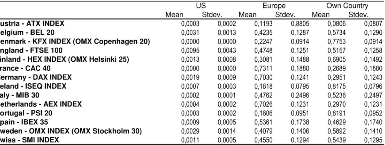
Table 3: Variance ratios – constant spillover model
The table reports the mean and standard deviation of the US, European, and own variance ratios for the constant spillover model:
Mean Stdev. Mean Stdev. Mean Stdev.
Austria - ATX INDEX 0,0003 0,0002 0,1193 0,8805 0,0806 0,0807
Belgium - BEL 20 0,0031 0,0013 0,4235 0,1287 0,5734 0,1290
Denmark - KFX INDEX (OMX Copenhagen 20) 0,0000 0,0000 0,2247 0,0914 0,7753 0,0914
England - FTSE 100 0,0095 0,0043 0,4748 0,1251 0,5157 0,1258
Finland - HEX INDEX (OMX Helsinki 25) 0,0013 0,0008 0,3081 0,1488 0,6905 0,1492
France - CAC 40 0,0000 0,0000 0,7311 0,1880 0,2689 0,1880
Germany - DAX INDEX 0,0019 0,0009 0,7030 0,1241 0,2951 0,1243
Ireland - ISEQ INDEX 0,0007 0,0003 0,1818 0,0795 0,8175 0,0796
Italy - MIB 30 0,0002 0,0001 0,4762 0,2496 0,5236 0,2497
Netherlands - AEX INDEX 0,0004 0,0002 0,7026 0,1231 0,2970 0,1231
Portugal - PSI 20 0,0003 0,0002 0,1806 0,0951 0,8191 0,0952
Spain - IBEX 35 0,0009 0,0005 0,5361 0,1738 0,4629 0,1740
Sweden - OMX INDEX (OMX Stockholm 30) 0,0029 0,0014 0,4079 0,1406 0,5892 0,1410
Swiss - SMI INDEX 0,0011 0,0005 0,4550 0,1294 0,5439 0,1295
US Europe Own Country
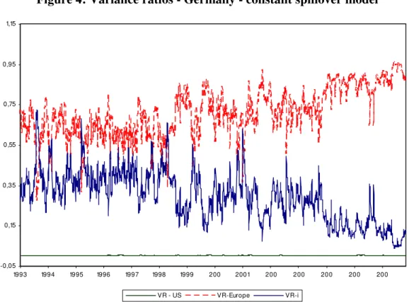
the results achieved. Finally, the purely local volatility effects are larger for Austria, Ireland and Portugal (means of 81.75%, 81.91% and 88%, respectively) than for the other countries (the means range between 27% and 78%). To all purposes of our study all the Non-EMU countries and the Non-EU country behave like EMU-member countries, which give an idea of how integrated the euro countries are. Figures 4 to 7 show the time series evolution of the variance ratios for Germany, UK (representing the non-EMU countries), Portugal and Spain. We chose these countries because Germany and the UK are a wide representation of the European stock markets, and the most liquid ones; and Portugal and Spain because of the interest that those two indexes bring to our study once we are in their financial space. The European variance ratio generally increases over the sample period for all countries except (again) Sweden and the UK, for which it appears to be stable.
Figure 4: Variance ratios - Germany - constant spillover model
-0,05 0,15 0,35 0,55 0,75 0,95 1,15
1993 1994 1995 1996 1997 1998 1999 200 2001 200 200 200 200 200
Figure 5: Variance ratios - UK - constant spillover model
-0,05 0,05 0,15 0,25 0,35 0,45 0,55 0,65 0,75 0,85 0,95
1993 1994 1995 1996 1997 1998 1999 200 2001 200 200 200 200 200
VR-US VR-Europe VR-i
Figure 6: Variance ratios - Portugal - constant spillover model
-0,05 0,15 0,35 0,55 0,75 0,95 1,15
1993 1994 1995 1996 1997 1998 1999 200 2001 200 200 200 200 200
Figure 7: Variance ratios - Spain - constant spillover model
-0,05 0,15 0,35 0,55 0,75 0,95 1,15
1993 1994 1995 1996 1997 1998 1999 200 2001 200 200 200 200 200
VR-US VR-Europe VR-i
The results regarding the relative size of volatility-spillover effects are in line with results from Baele (2005). Our conclusions are contrary to the ones from Ilmanen (1995) who states that world factors are more important than local factors.
Europe Spillover Model
Continuing with the framework proposed by Charlotte Christiansen (2005), we will now report the results from estimating the euro spillover model, which tries to make a register of the changes brought by the introduction of the European single currency. This effect is achieved by the introduction of a dummy variable, i.e. by letting the spillover parameters take on different values before and after the introduction of the euro, cf. equation (16).
To do so we keep the US returns specifications equal to the constant spillover model,
, 0, 1, , 1 ,
US t US US US t US t
R c c R e where eUS t, has mean 0 and conditional variance,
2 2 2
, , 1 , 1
US t US US US te US US t . But now we will change the European return in order to
be described by the following extended AR(1),
, 0, 1, , 1 ( 0, 1, ) , 1 ( 0, 1, ) , ,
E t E E E t E t US t E E t US t E t
R c c R D R D e e
where eE t, has mean 0
and conditional variance, E t2, E E E te2, 1 E E t2, 1. On the other hand the Country i
returns assume the following specification for country i (i=1,…,N),
, 0, 1, , 1 ( 0, 1, ) , 1 ( 0, 1, ) , 1 ( 0, 1, ) , ( 0, 1, ) , ,
i t i i i t i i t US t i i t E t i i t US t i i t E t i t
R c c R D R D R D e D e e wh
ere ei t, has mean 0 and conditional variance:
2 2 2
, , 1 , 1
At this point we also going to report the results about the mean and standard deviation of the US, European, and own variance ratios for the euro spillover model,
2 2
0, 1, ,
,
,
( i i t) US t US
i t
i t
D VR
h
,
2 2
0, 1, ,
,
,
( i i t) E t E
i t
i t
D VR
h
, and , 1 , ,
i US E
i t i t i t
VR VR VR
., where
,
US t and E t, are the conditional volatility of the US and European idiosyncratic shock,
respectively and hi t, is the conditional variance of the unexpected return of country i. Table
Table 4: Euro spillover model
The table reports the results from estimating the euro spillover model. Estimated parameters and standard errors below - *, §, #, indicates that the value is significant at a 1%, 5% or 10% level of significance, respectively.
USA - S&P 500 0,000526* 0,002772
0,000126 0,001704
Europe - DJ EURO STOXX 50 0,000526* -0,147940* 0,509626* -0,087977§ 0,309643* 0,260583*
0,000129 0,015695 0,029559 0,037391 0,027421 0,036137
Austria - ATX INDEX 0,000513* 0,071980* 0,411022* -0,214712* -0,046319# 0,002696 0,123853* 0,008494 0,548738* -0,321433*
0,000124 0,018683 0,033834 0,038931 0,026243 0,029113 0,031826 0,037364 0,028332 0,033152
Belgium - BEL 20 0,000609* 0,065905* 0,312367* -0,034174 -0,052343§ -0,040435# 0,242061* 0,107631* 0,535006* 0,055753§
0,000090 0,018631 0,020750 0,026629 0,020855 0,024002 0,017698 0,022739 0,019092 0,023495
Denmark - KFX INDEX (OMX Copenhagen 20) 0,000533* 0,066760* 0,320643* -0,001136 -0,070356§ -0,015581 0,178900* 0,058390# 0,535950* -0,106883*
0,000124 0,018684 0,025838 0,035496 0,028631 0,034041 0,021908 0,033191 0,024911 0,031289
England - FTSE 100 0,000376* -0,057500* 0,308399* 0,043697# -0,061389* -0,030489 0,319619* 0,073191* 0,559919* 0,053882§
0,000082 0,017972 0,019716 0,024259 0,019607 0,020062 0,018637 0,022277 0,019557 0,022980
Finland - HEX INDEX (OMX Helsinki 25) 0,000731* 0,037927# 0,645006* -0,019095 -0,129480* -0,047658 0,283467* 0,228997* 0,713582* 0,166984*
0,000163 0,020112 0,036271 0,047277 0,034147 0,039322 0,044020 0,054625 0,032840 0,041991
France - CAC 40 0,000534* -0,127928* 0,440579* -0,014503 -0,046984# 0,035011 0,379352* 0,141641* 0,980417* -0,029236
0,000052 0,017781 0,022006 0,023300 0,027485 0,021689 0,019633 0,020762 0,017766 0,019466
Germany - DAX INDEX 0,000652* -0,173307* 0,600488* -0,213532* 0,079876* -0,050401# 0,242154* 0,406137* 0,961667* 0,051140§
0,000066 0,017223 0,020118 0,023136 0,029422 0,026407 0,023144 0,025412 0,021511 0,023951
Ireland - ISEQ INDEX 0,000527* 0,046620§ 0,438553* -0,101338§ 0,018434 -0,070919* 0,134538* 0,082676* 0,352732* 0,013292
0,000110 0,018870 0,032244 0,040244 0,021540 0,027211 0,021692 0,031695 0,024023 0,030813
Italy - MIB 30 0,000542* -0,019243 0,435509* -0,196006* -0,115107* 0,046488 0,316572* 0,117705* 0,987333* -0,238374*
0,000088 0,018455 0,035956 0,038392 0,036358 0,033334 0,039347 0,040876 0,030514 0,032866
Netherlands - AEX INDEX 0,000559* -0,042421§ 0,478068* -0,065968* -0,126608* 0,046469§ 0,329700* 0,177410* 0,840322* 0,070137*
0,000066 0,018512 0,017620 0,021005 0,026289 0,022193 0,018238 0,021056 0,018006 0,020377
Portugal - PSI 20 0,000368* 0,142479* 0,152165* 0,049621 0,032640 -0,110377* 0,046055 0,157954* 0,325365* 0,023515
0,000100 0,020448 0,027595 0,033173 0,026058 0,029265 0,039156 0,042137 0,024194 0,029782
Spain - IBEX 35 0,000692* 0,034473# 0,382700* -0,046838 -0,141956* 0,000434 0,367331* 0,086985* 0,886624* -0,095916*
0,000088 0,020228 0,025944 0,029532 0,029861 0,026938 0,026112 0,029068 0,034970 0,036873
Sweden - OMX INDEX (OMX Stockholm 30) 0,000781* -0,040394§ 0,490405* -0,020546 -0,131068* 0,030709 0,356465* 0,111420* 0,774169* 0,020978
0,000127 0,018167 0,031778 0,039593 0,027339 0,029141 0,027203 0,033954 0,027401 0,034770
Swiss - SMI INDEX 0,000604* 0,012556 0,377603* -0,061143§ -0,123026* 0,025211 0,289885* 0,082708* 0,742399* -0,095949*
0,000096 0,018091 0,023455 0,028882 0,024409 0,024600 0,022739 0,027336 0,020757 0,026179
0,i
The estimates of the GARCH parameters ( i, i, and i) are not reported because they are similar to the results of the constant spillover model. The univariate model for the US return is identical to that of the constant spillover model; for convenience the results are repeated in the first row of Table 4.
The second step of the estimation concerns the return of the DJ EURO STOXX 50, cf. the second row of Table 4. The joint hypothesis of no spillover changes after the euro is strongly rejected; the robust Wald test for the hypothesis H0: 1, 1,E 0 results in a p-value equal to 0%.
The subsequent results are robust to including or excluding euro changes in the spillover parameters. Thus, we continue with the dummy variable in the specification for the European return.
In the third step of the estimation, we investigate the effect of the euro on the mean-spillover effects and the volatility-mean-spillover effects from the US and European stock markets to the European stock markets cf. the bottom rows of Table 4. As for the constant spillover model, we only find spotted evidence of mean spillover effects. For the period before the euro there are only mean-spillover effects for a few countries, ^
0,i and ^
There are strong indications of both US and European volatility-spillover effects. For the period before the euro the US volatility-spillover effects as well as the European volatility-spillover effects are significant, i.e. 0,i and 0,i are significant, the only
parameter that is not significant at this point is the Portuguese PSI 20’s US volatility
spillover. In addition, the volatility-spillover effects are significantly different after the euro; the robust Wald test for the hypothesis H0: 1,i 1,i 0 is rejected for all countries. There are also significant volatility spillover effects after the euro;H0: 0,i 1,i 0,i 1,i 0 is rejected for all i.
We tried to demonstrate how the introduction of the euro has significantly changed the volatility spillover effects into European stock markets.
The following commonalities are observed in our study. The US volatility-spillover effects before the euro are found to be stronger than the effects estimated by the constant
spillover model, i.e. ^ ^
0,i i
. The US volatility-spillover effects weaken by the euro
(^ ^
1,i 0,i
) and are stronger than estimated by the constant spillover model, ^ ^ ^
0,i 1,i i .
In contrast, the European volatility-spillover effects before the euro are found to be weaker than estimated by the constant spillover model, for half of the counties under our scope, ^ ^
0,i i
. After the euro, the effects of European volatility spillover are
strengthened ( ^
1,
0 i
) and are stronger than estimated by the constant spillover model,
^ ^ ^
0,i 1,i i
Table 5 presents the mean of the variance ratios. In the first sub period the average US variance ratios are smaller than in the second sub period. Compared to the constant spillover model, the mean of the US variance ratio has increased from 0-1% to 2-16%, because the sample period before the euro is longer than the sample period after the euro.
Table 5: Variance ratios – euro spillover model
The table reports the mean and standard deviation of the US, European, and own variance ratios for the euro spillover model:
Mean Stdev. Mean Stdev. Mean Stdev.
Austria - ATX INDEX 0,0213 0,0170 0,1488 0,1071 0,8299 0,1080
Belgium - BEL 20 0,1097 0,0502 0,3769 0,1151 0,5134 0,1323
Denmark - KFX INDEX (OMX Copenhagen 20) 0,0479 0,0286 0,2220 0,0890 0,7301 0,0969
England - FTSE 100 0,1544 0,0644 0,4033 0,1115 0,4423 0,1340
Finland - HEX INDEX (OMX Helsinki 25) 0,0761 0,0483 0,2812 0,1337 0,6427 0,1652
France - CAC 40 0,1561 0,0857 0,6166 0,1320 0,2273 0,1736
Germany - DAX INDEX 0,1568 0,1166 0,5853 0,0895 0,2578 0,1301
Ireland - ISEQ INDEX 0,0460 0,0281 0,1728 0,0737 0,7812 0,0877
Italy - MIB 30 0,1183 0,0849 0,4411 0,1724 0,4405 0,2284
Netherlands - AEX INDEX 0,1508 0,0786 0,5882 0,1038 0,2610 0,1299
Portugal - PSI 20 0,0380 0,0371 0,1626 0,0855 0,7994 0,1109
Spain - IBEX 35 0,1323 0,0686 0,4809 0,1272 0,3868 0,1575
Sweden - OMX INDEX (OMX Stockholm 30) 0,1094 0,0532 0,3680 0,1223 0,5226 0,1477
Swiss - SMI INDEX 0,1099 0,0569 0,4205 0,1046 0,4696 0,1184
US Europe Own Country
The average European variance ratios are smaller in the last sub period than in the first sub period. Therefore, the means of the European variance ratios tend to be smaller in the euro spillover model than in the constant spillover model. The purely local volatility effects are, in general, smaller after the introduction of the euro. The average local variance ratio has decreased from 57% to 52%. The tendencies are also seen in the plots of the variance ratios for the example country Germany in Figure 8. Thus, after the introduction of the euro there is much more sensitivity from the own stock markets to the changes that come in from the European stock market and less room for local effects.