Efficient Market Hypothesis in European Stock Markets

Carlos Pestana Barros & Nicolas Peypoch

A Comparative Analysis of Productivity Change in Italian and Portuguese Airports

WP 006/2007/DE _________________________________________________________

Maria Rosa Borges

Efficient Market Hypothesis in European Stock Markets

WP 20/2008/DE/CIEF _________________________________________________________

Department of Economics

W

ORKING

P

APERS

ISSN Nº0874-4548

School of Economics and Management

Efficient Market Hypothesis in European Stock Markets

M

ARIA

R

OSA

B

ORGES

Technical University of Lisbon Instituto Superior de Economia e Gestão

Department of Economics Rua Miguel Lupi, 20, 1249-078 Lisbon

e-mail: mrborges@iseg.utl.pt

Efficient Market Hypothesis in European Stock Markets

Abstract

This paper reports the results of tests on the weak-form market efficiency applied to stock market indexes of France, Germany, UK, Greece, Portugal and Spain, from January 1993 to December 2007. We use a serial correlation test, a runs test, an augmented Dickey-Fuller test and the multiple variance ratio test proposed by Lo and MacKinlay (1988) for the hypothesis that the stock market index follows a random walk. The tests are performed using daily and monthly data for the whole period and for the period of the last five years, i.e., 2003 to 2007. Overall, we find convincing evidence that monthly prices and returns follow random walks in all six countries. Daily returns are not normally distributed, because they are negatively skewed and leptokurtic. France, Germany, UK and Spain meet most of the criteria for a random walk behavior with daily data, but that hypothesis is rejected for Greece and Portugal, due to serial positive correlation. However, the empirical tests show that these two countries have also been approaching a random walk behavior after 2003. (JEL G14; G15)

Introduction

Efficient market theory and the random walk hypothesis have been major issues in

financial literature, for the past thirty years. While a random walk does not imply that a

market can not be exploited by insider traders, it does imply that excess returns are not

obtainable through the use of information contained in the past movement of prices. The

validity of the random walk hypothesis has important implications for financial theories and

investment strategies, and so this issue is relevant for academicians, investors and regulatory

authorities. Academicians seek to understand the behavior of stock prices, and standard

risk-return models, such as the capital asset pricing model, depend of the hypotheses of normality

or random walk behavior of prices. For investors, trading strategies have to be designed

taking into account if the prices are characterized by random walks or by persistence in the

short run, and mean reversion in the long run. Finally, if a stock market is not efficient, the

negative effects for the overall economy. Evidence of inefficiency may lead regulatory

authorities to take the necessary steps and reforms to correct it.

Since the seminal work of Fama (1970), several studies show that stock price returns do

not follow a random walk and are not normally distributed, including Fama and French

(1988) and Lo and MacKinlay (1988), among many others. The globalization markets

spawned interest on the study of this issue, with many studies both on individual markets and

regional markets, such as Latin America (Urrutia 1995, Grieb and Reyes 1999), Africa (Smith

at al. 2002, Magnusson and Wydick 2002), Asia (Huang 1995, Groenewold and Ariff 1998),

Middle East (Abraham et al. 2002) and Europe (Worthington and Higgs 2004), several

reporting unconformity with random walk behavior. The list is too extensive for a

comprehensive survey, which is beyond the purpose of this study.

Recent studies of weak-form efficiency of European markets include Smith and Ryoo

(2003) and Worthington and Higgs (2004). Smith and Ryoo (2003) use a variance ratio test on

weekly data for five European indexes, covering April 1991 to August 1998, and reject the

random walk hypothesis for Greece, Hungary, Poland and Portugal but find that Turkey

follows a random walk.

Worthington and Higgs (2004) conduct a very detailed study of twenty European

countries, from August 1995 to May 2003, applying multiple testing procedures, including

serial correlation test, runs test, augmented Dickey Fuller test and a variance ratio test. They

find that all indexes are not well explained by the normal distribution, and only five countries

meet the most stringent criteria for a random walk, namely, Germany, Ireland, Portugal,

Sweden and the United Kingdom, while France, Finland, the Netherlands, Norway and Spain

meet only some of the requirements for a random walk.

The main contribution of this paper is to add to international evidence on the random

Southern European less developed capital markets (Greece, Portugal and Spain), with very

recent data, up until December 2007. The first three countries are included also as a control

for the quality of the data and of the tests, as we would expect, ex-ante, for the empirical

evidence to be more favorable to the random walk hypothesis in those countries’ markets. We

follow the Worthington and Higgs (2004) approach of using several different tests, to avoid

that a spurious result from one of the tests might affect our conclusions. We will look at the

global results of all four tests, to draw our conclusions.

Methodology

Serial correlation of returns

An intuitive test of the random walk for an individual time series is to check for serial

correlation. If the stock market indexes returns exhibit a random walk, the returns are

uncorrelated at all leads and lags. We perform least square regressions of daily and monthly

returns on lags one to ten of the return series. To test the joint hypothesis that all serial

coefficients ρ

( )

t are simultaneously equal to zero, we apply the Box-Pierce Q statistic:

( )

∑

= = m

t BP n t

Q

1

ˆ

ρ (1)

where QBP is asymptotically distributed as a chi-square with m degrees of freedom, n is the

number of observations, and m is the maximum lag considered (in this study, m equals ten).

We also use a Ljung-Box test, which provides a better fit to the chi-square distribution, for

small samples:

(

)

_∑

( )

= −

+

= m

t LB

t n

t n

n Q

1 2

ˆ

Runs test

To test for serial independence in the returns we also employ a runs test, which

determines whether successive price changes are independent of each other, as should happen

under the null hypothesis of a random walk. By observing the number of runs, that is, the

successive price changes (or returns) with the same sign, in a sequence of successive price

changes (or returns), we can test that null hypothesis. We consider two approaches: in the

first, we define as a positive return (+) any return greater than zero, and a negative return (-) if

it is below zero; in the second approach, we classify each return according to its position with

respect to the mean return of the period under analysis. In this last approach, we have a

positive (+) each time the return is above the mean return and a negative (-) if it is below the

mean return. This second approach has the advantage of allowing for and correcting the effect

of an eventual time drift in the series of returns. Note that this is a non-parametric test, which

does not require the returns to be normally distributed. The runs test is based on the premise

that if price changes (returns) are random, the actual number of runs (R) should be close to

the expected number of runs (µ_R).

Let n₊ and n₋ be the number of positive returns (+) and negative returns (-) in a sample

with n observations, wheren=n₊ +n₋. For large sample sizes, the test statistic is

approximately normally distributed:

( )

0,1

N R

Z

R R ≈

− =

σ µ

(3)

where = 2 + − +1

n n n

R

µ and

(

)

(

1

)

2 2

2 − − = + − + −

n n

n n n n n

R

Unit Root Tests

Our third test is the augmented Dickey-Fuller (ADF) test which is used to test the

existence of a unit root in the series of price changes in the stock index series, by estimating

the following equation through OLS:

∑

= −

− + ∆ +

+ + =

∆ q

i

it i it i t

t t P P

P

1 1 0 1

0 α ρ ρ ε

α (4)

where P_t is the price at time t, and ∆P_t =P_t−P_t−1, ρ_i are coefficients to be estimated, q is

the number of lagged terms, t is the trend term, α_i is the estimated coefficient for the trend,

0

α is the constant, and ε is white noise. The null hypothesis of a random walk is H₀:ρ₀=0

and its alternative hypothesis is H₁:ρ₀ ≠0. Failing to reject H₀ implies that we do not reject

that the time series has the properties of a random walk. We use the critical values of

MacKinnon (1994) in order to determine the significance of the t-statistic associated withρ₀.

Variance Ratio Tests

An important property of the random walk is explored by our final test, the variance

ratio test. If Pt is a random walk, the ratio of the variance of the qth difference scaled by q to

the variance of the first difference tends to equal one, that is, the variance of the q-differences

increases linearly in the observation interval,

( )

( )

_{( )}

1

2 2

σ

σ q

q

VR = (5)

where σ2

( )

q is 1/q the variance of the q-differences and σ2

( )

1 is the variance of the first

differences. Under the null hypothesis VR(q) must approach unity. The following formulas

are taken from Lo and MacKinlay [1988], who propose this specification test, for a sample

( )

(

)

2

2 1

∑

_ˆ

= − − − = nq q t q t t P q

P m

q µ

σ (6)

where

(

)

_

     ₋ + − = nq q q nq q

m 1 1 and µˆ is the sample mean of

(

P_t−P_t−1

)

: ˆ 1

(

P P₀

)

nq nq−

=

µ and

( ) ( ) (

)

2

1 1 2 _ˆ 1 1 1

∑

= − − − − = nq t t t P P nq µ

σ (7)

Lo and MacKinlay (1988) generate the asymptotic distribution of the estimated variance

ratios and propose two test statistics, Z

( )

q andZ*

( )

q , under the null hypothesis of

homoskedastic increments random walk and heteroskedastic increments random walk

respectively. If the null hypothesis is true, the associated test statistic has an asymptotic

standard normal distribution. Assuming homoskedastic increments, we have

( )

( )

_{( )}

1 N

( )

0,1

q q VR q Z o ≈ − =

φ (8)

where

( )

(

)(

)

( )

2 1 3 1 1 2 2       − − = nq q q q q o

φ . Assuming heteroskedastic increments, the test statistic is

( )

( )

_{( )}

1

( )

0,1

* N q q VR q Z e ≈ − =

φ (9)

where

( )

2 1 1 1 ˆ 1 4 _            ₋ =

∑

− = q t t e q t q δ

φ and

(

) (

)

(

)

2

1 2 1 1 2 1 2 1 ˆ ˆ ˆ ˆ       − − − − − − =

∑

∑

= − + = − − −− nq j j j nq t j t j t j j j t P P P P P P µ µ µ

δ .

which is robust under heteroskedasticity, hence can be used for a longer time series analysis.

The procedure proposed by Lo and MacKinlay (1988) is devised to test individual variance

ratio tests for a specific q-difference, but under the random walk hypothesis, we must have

( )

q =1

VR for all q. A multiple variance ratio test is proposed by Chow and Denning (1993).

associated with the set of aggregation intervals

{

q_ii=1,2,...,m

}

. Under the random walk

hypothesis, there are multiple sub-hypotheses:

( )

0 :

0i Mr qi =

H for i=1,2,...,m

( )

0 :

1i Mr qi ≠

H for any i=1,2,...,m

The rejection of any or more H_0i rejects the random walk null hypothesis. In order to

facilitate comparison of this study with previous research (Lo and MacKinlay, 1988 and

Campbell et al. 1997) on other markets, the q is selected as 2, 4, 8, and 16. For a set of test

statistics

{

Z

( )

q_i i=1,2,...,m

}

, the random walk hypothesis is rejected if any one of the VR

( )

q_i

is significantly different than one, so only the maximum absolute value in the set of test

statistics is considered. The Chow and Denning (1993) multiple variance ratio test is based on

the result:

( )

( )

(

)

(

)

{

max Z q₁ ,...,Z q ≤SMM α;m;T

}

≥1−α

PR _m (10)

in which SMM

(

α;m;T

)

is the upper α point of the Studentized Maximum Modulus (SMM)

distribution with parameters m and T (sample size) degrees of freedom. Asymptotically,

(

; ;

)

*₂

lim_T→∞SMM α m ∞ =Z_α (11)

where Z_α*₂ is standard normal with

(

)

m

1 *

1

1 α

α = − − . Chow and Denning (1993) control the

size of the multiple variance ratio test by comparing the calculated values of the standardized

test statistics, either Z

( )

q or Z*

( )

q _{with the SMM critical values. If the maximum absolute}

value of , say, Z

( )

q is greater than the critical value at a predetermined significance level then

The Data

Our data are daily closing values of stock market indexes for France, Germany, UK,

Greece, Portugal and Spain*, chosen as representative for each of these markets. The source of all data is Reuters, and it includes observations from 1 January 1993 to 31 December 2007,

during which the markets were very volatile, especially in the case of Greece, as shown

visually in Figure 1.

FIGURE 1

Stock Market Indexes – Closing Prices – 1993 to 2007

We apply the empirical tests to the whole 15-year period, but also to a smaller period

of five years, from 1 January 2003 to 31 December 2007. The testing of different periods has

the advantage of allowing for structural changes, so that the market may follow a random

walk in some period while in other periods that hypothesis may be rejected. A similar

Warsaw Stock Exchange. We are particularly interested in examining the last five years, from

January 2003 to December 2007, because it has not been covered by previous studies.

We use the daily closing prices to compute monthly data. For the monthly price series,

we use the observations of day 15 of each month. In case of a missing observation on day 15,

we use day 14. If day 14 is missing, we use day 16. If day 16 is missing we use day 13, and so

on. From country samples of around 3880 daily observations, we generate 180 monthly

observations for the whole period. The returns are computed as the logarithmic difference

between two consecutive prices in a series. Table 1 shows the descriptive statistics for the

returns of the stock market indexes.

TABLE 1

Descriptive statistics for the returns of the stock market indexes: January 1993 to December 2007

France 1993-2007

Germany 1993-2007

UK 1993-2007

Greece 1993-2007

Portugal 1993-2007

Spain 1993-2007

France 2003-2007

Germany 2003-2007

UK 2003-2007

Greece 2003-2007

Portugal 2003-2007

Spain 2003-2007

Daily Returns

Observations 3878 3878 3878 3878 3878 3878 1292 1292 1292 1292 1292 1292 Mean return 0,0003 0,0004 0,0002 0,0005 0,0004 0,0005 0,0005 0,0008 0,0004 0,0008 0,0006 0,0007 Annual. return 0,0739 0,1124 0,0542 0,1406 0,0992 0,1279 0,1243 0,2194 0,1003 0,2337 0,1683 0,1953 Maximum 0,0700 0,0755 0,0590 0,0766 0,0694 0,0632 0,0700 0,0709 0,0590 0,0497 0,0384 0,0405 Minimum -0,0768 -0,0887 -0,0589 -0,0962 -0,0959 -0,0734 -0,0583 -0,0634 -0,0492 -0,0611 -0,0463 -0,0424 St. Deviation 0,0130 0,0141 0,0103 0,0152 0,0097 0,0126 0,0107 0,0120 0,0089 0,0103 0,0068 0,0094 Studentiz. range 11,3143 11,6754 11,4814 11,3651 17,0475 10,8074 11,9752 11,1596 12,1673 10,8023 12,3821 8,8507 Skewness -0,1068 -0,2685 -0,2145 -0,1102 -0,6442 -0,2104 -0,0588 -0,0461 -0,1375 -0,3197 -0,3690 -0,3115 Excess Kurtosis 2,8273 3,6514 3,1670 4,3767 8,2305 3,0243 3,8577 3,9134 4,0828 2,5914 3,8434 2,3142 Jarque-Bera 1299** 2201** 1650** 3103** 11214** 1506** 801,9** 824,9** 901,4** 383,5** 824,5** 309,2** JB p-value 0,0000 0,0000 0,0000 0,0000 0,0000 0,0000 0,0000 0,0000 0,0000 0,0000 0,0000 0,0000

Monthly Returns

Observations 179 179 179 179 179 179 60 60 60 60 60 60 Mean return 0,0063 0,0092 0,0047 0,0111 0,0084 0,0102 0,0100 0,0158 0,0083 0,0172 0,0134 0,0156 Annual. return 0,0778 0,1155 0,0577 0,1415 0,1050 0,1293 0,1268 0,2072 0,1048 0,2265 0,1736 0,2037 Maximum 0,1350 0,1649 0,1008 0,4198 0,1695 0,1526 0,0715 0,1649 0,0838 0,1194 0,0797 0,1053 Minimum -0,2327 -0,2817 -0,1478 -0,2578 -0,2040 -0,2361 -0,1169 -0,1312 -0,0948 -0,1441 -0,0759 -0,0948 St. Deviation 0,0507 0,0588 0,0413 0,0846 0,0558 0,0574 0,0365 0,0498 0,0311 0,0511 0,0354 0,0426 Studentiz. range 7,2540 7,6017 6,0175 8,0123 6,6992 6,7679 5,1658 5,9479 5,7455 5,1521 4,3926 4,6972 Skewness -1,0511 -1,0124 -0,8951 0,4718 -0,3887 -0,7244 -1,3417 -0,5157 -0,7291 -0,7719 -0,6215 -0,2976 Excess Kurtosis 2,8865 3,1355 2,0670 3,0764 1,2182 2,1915 2,7620 1,6616 1,7221 0,8207 -0,1467 -0,0729 Jarque-Bera 95,10** 103,9** 55,77** 77,22** 15,58** 51,47** 37,07** 9,56** 12,73** 7,642* 3,917 0,899 JB p-value 0,0000 0,0000 0,0000 0,0000 0,0004 0,0000 0,0000 0,0084 0,0017 0,0219 0,1411 0,6380

Notes: The Jarque-Bera test is a goodness-of-fit measure of departure from normality, based on the sample kurtosis and skewness, and is distributed as a chi-squared with two degrees of freedom. The null hypothesis is a joint hypothesis of both the skewness and excess kurtosis being 0, since samples from a normal distribution have an expected skewness of 0 and an expected excess kurtosis of 0. As the definition of JB shows, any deviation from this increases the JB statistic.

* Null hypothesis rejection significant at the 5% level. ** Null hypothesis rejection significant at the 1% level.

The daily returns are negatively skewed in all six countries both for the period

in both periods, indicating that the distributions of returns are leptokurtic, thus having higher

peaks than would be expected from normal distributions. The only exceptions are Portugal

and Spain, in the last five year period, with a negative excess kurtosis. The Jarque-Bera

statistic rejects the hypothesis of a normal distribution of daily returns in all countries and

periods, at a significance level of 1%, although this statistic is lower for all countries in the

period 2003-2007.

For the period 1993-2007, the evidence from monthly returns is consistent with the

evidence from daily returns, showing negative skewness and positive excess kurtosis, and a

rejection of normality by the Jarque-Bera statistic. Note, however, that this statistic is much

closer to zero than in the case of daily returns, thus evidencing a milder departure from the

normal distribution. In the last five years, the departure from normality is further reduced for

all countries, and in the case of Portugal and Spain we can no longer reject that monthly

returns follow a normal distribution.

Results

Serial Correlation

The results for the tests on serial correlation, Box-Pierce and Ljung-Box statistics are

presented in Table 2, for daily and monthly returns.

The evidence of positive serial correlation of lag 1 of daily returns is only present in

Greece and Portugal, both for the whole period and for the last five years, which is

inconsistent with the random walk hypothesis. However, the coefficients of 0.14 and 0.15,

which we find for these two countries in the whole sample, are lower in the last five years,

0.07 and 0.06. All other countries do not show positive serial correlation, as most lag

coefficients are not statistically significant different from zero and, when they are significant,

cannot reject the joint significance of the coefficients for lags 1 to 10, except in the case of

France, and also Greece and Spain, for the last five years period.

TABLE 2

Serial correlation coefficients and Q-statistics for Returns of the stock market indexes: January 1993 to December 2007

France 1993-2007

Germany 1993-2007

UK 1993-2007

Greece 1993-2007

Portugal 1993-2007

Spain 1993-2007

France 2003-2007

Germany 2003-2007

UK 2003-2007

Greece 2003-2007

Portugal 2003-2007

Spain 2003-2007

Daily Returns

Observations 3868 3868 3868 3868 3868 3868 1282 1282 1282 1282 1282 1282

Lag 1 -0,010 -0,019 -0,010 0,143** 0,151** 0,035* -0,025 -0,057* -0,102** 0,071* 0,063* -0,036 Lag 2 -0,001 -0,008 -0,041* -0,020 -0,002 -0,037* 0,010 0,045 0,024 0,006 0,010 0,017 Lag 3 -0,026 -0,015 -0,068** 0,000 0,020 -0,029 -0,017 0,004 -0,044 0,005 0,030 -0,022 Lag 4 0,001 0,010 0,004 -0,005 0,037* 0,008 0,001 -0,015 0,005 0,003 0,031 0,016 Lag 5 -0,014 -0,028 -0,046** 0,004 -0,012 -0,005 -0,004 -0,077** -0,057* -0,008 -0,058* -0,009 Lag 6 -0,003 -0,044** -0,038* 0,020 -0,016 -0,022 0,006 -0,039 -0,019 0,024 0,009 -0,034 Lag 7 -0,021 -0,004 -0,015 -0,019 0,025 0,004 -0,023 -0,092** -0,111** -0,029 0,044 -0,072* Lag 8 0,016 0,025 0,035* 0,026 0,041* 0,029 0,014 0,053 -0,012 0,020 0,032 0,043 Lag 9 -0,017 -0,004 0,012 -0,016 -0,020 -0,008 -0,024 -0,019 0,008 -0,028 -0,072** -0,033 Lag 10 -0,006 -0,026 -0,043** 0,004 0,046** 0,032* -0,004 -0,053 -0,046 0,006 0,068* -0,050

Box-Pierce Stat. 7,72 18,64* 52,01** 87,20** 114,8** 22,87* 3,07 35,41** 40,24** 9,91 28,40** 18,04

p-value 0,656 0,045 0,000 0,000 0,000 0,011 0,980 0,000 0,000 0,448 0,002 0,054 Ljung-Box Stat. 7,74 18,68* 52,11** 87,28** 114,9** 22,91* 3,08 35,62** 40,45** 9,95 28,59** 18,16

p-value 0,655 0,045 0,000 0,000 0,000 0,011 0,979 0,000 0,000 0,445 0,001 0,052 Monthly Returns

Observations 169 169 169 169 169 169 50 50 50 50 50 50

Lag 1 0,075 0,098 -0,107 0,043 0,224** 0,046 0,050 -0,048 -0,136 0,088 0,255 -0,245 Lag 2 0,087 0,094 0,046 0,068 -0,019 -0,030 -0,145 -0,035 -0,304 -0,309* -0,198 0,023 Lag 3 0,077 0,003 0,006 0,113 0,062 0,055 -0,056 -0,092 -0,180 0,010 -0,158 -0,161 Lag 4 -0,136 -0,064 -0,054 -0,026 -0,043 -0,019 -0,378* -0,367* -0,289 -0,377* -0,104 -0,462* Lag 5 0,093 0,111 0,082 -0,133 0,000 -0,058 0,433* 0,267 0,106 -0,053 0,052 -0,123 Lag 6 0,024 0,011 -0,009 -0,066 0,018 -0,053 -0,249 -0,145 -0,176 -0,185 -0,178 -0,025 Lag 7 -0,049 -0,093 0,004 0,184* 0,047 0,087 -0,140 -0,105 -0,196 -0,234 -0,104 -0,105 Lag 8 -0,029 -0,011 -0,018 0,044 -0,044 -0,035 0,062 -0,074 0,121 -0,087 -0,068 -0,059 Lag 9 0,232** 0,174* 0,149 0,096 0,069 0,157* 0,226 0,079 0,026 0,085 -0,011 -0,083 Lag 10 0,010 -0,071 0,011 -0,086 0,043 0,032 -0,309 -0,260* -0,105 -0,277 -0,071 -0,079

Box-Pierce Stat. 17,54 13,34 7,77 15,97 11,38 7,96 29,45** 16,50 16,69 21,43* 9,75 17,17

p-value 0,063 0,205 0,651 0,100 0,328 0,633 0,001 0,086 0,082 0,018 0,463 0,071 Ljung-Box Stat. 18,46* 14,01 8,14 16,77 11,69 8,42 34,89** 19,47* 18,97* 25,01** 10,87 19,35*

p-value 0,048 0,172 0,615 0,080 0,306 0,588 0,000 0,035 0,041 0,005 0,368 0,036

Notes: Both the Box-Pierce statistic and the Ljung-Box statistic test the null hypothesis of overall zero serial correlation coefficients for lags 1 through 10, and are distributed as a chi-square distribution with ten degrees of freedom. For small samples, the Ljung-Box statistic provides a finite-sample correction that yields a better fit to the chi-square distribution. * Null hypothesis rejection significant at the 5% level. ** Null hypothesis rejection significant at the 1% level.

The evidence of serial correlation decays as the lag length increases, and it virtually

disappears for the monthly data. This means that the larger the interval of the observations of

prices, the less important is the lagged price for explaining future prices. This is consistent

with the findings of several other studies including Fama (1965), Panas (1990) and Ma and

Another interesting aspect of the data is that four countries show negative serial correlation in

the lag of 4 months, when we consider only the behavior in the last five years.

Taken together, the evidence from this test tends to refute more strongly the random

walk hypothesis only in Greece and Portugal, due to the presence of positive serial correlation

in lag 1. However, we should be cautious in the interpretation of these results, as they assume

normality, which we have shown that is not a valid assumption for the distribution of daily

and monthly returns of all six stock market indexes, in the period 1993 to 2007.

Runs Test

The results of the runs test, which do not depend on normality of returns, are presented

in Table 3, for daily and monthly returns.

Considering the period 1993-2007, the number of runs is significant less than the

expected number of runs both for Portugal and Greece, using daily returns which is consistent

with a positive serial correlation of returns and clearly rejecting the random walk hypothesis.

For Portugal this hypothesis is also rejected using monthly returns. The random walk

hypothesis is not rejected for France, Germany, UK and Spain, using either daily or monthly

returns. In fact, the number of runs even exceeds the expected number of runs in the case of

France, in the daily data.

In the more recent period of five years, between 2003 and 2007, the daily data for

France refutes the random walk hypothesis, but in this case because the number of runs

clearly exceeds the number of runs we would expect to find, if prices followed a random

walk. The UK, Germany and Spain also show more runs than expected, but this only

significant for these last two countries. Greece shows again less runs than expected, more

noticeably when returns are defined relatively to the mean return. The daily data does not

the last five years are compatible with a random walk. The only country where the null

hypothesis is never rejected by the runs test is the UK.

TABLE 3

Runs tests for daily and monthly returns of the stock markets indexes: January 1993 to December 2007

France 1993-2007 Germany 1993-2007 UK 1993-2007 Greece 1993-2007 Portugal 1993-2007 Spain 1993-2007 France 2003-2007 Germany 2003-2007 UK 2003-2007 Greece 2003-2007 Portugal 2003-2007 Spain 2003-2007

Panel A: positive/negative daily returns defined relative to zero

n+ 2050 2146 2080 2069 2114 2159 692 731 709 742 727 744

n- 1828 1732 1798 1809 1764 1719 599 560 582 549 564 547

R 1953 1914 1920 1704 1733 1891 700 661 670 601 620 673

R

µ 1933,6 1917,9 1929,7 1931,3 1924,2 1915,0 643,2 635,2 640,3 632,1 636,2 631,5

R

σ 31,031 30,778 30,968 30,993 30,879 30,732 17,865 17,643 17,784 17,557 17,672 17,540

Z 0,624 -0,127 -0,315 -7,333** -6,192** -0,782 3,182** 1,464 1,673 -1,770 -0,917 2,368*

p-value 0,533 0,899 0,753 0,000 0,000 0,434 0,001 0,143 0,094 0,077 0,359 0,018 Panel B: positive/negative daily returns defined relative to the mean return

n+ 1930 1994 1937 1847 1887 1962 658 665 656 643 653 668

n- 1948 1884 1941 2031 1991 1916 633 626 635 648 638 623

R 1977 1999 1940 1736 1765 1936 714 708 680 595 654 682

R

µ 1940,0 1938,4 1940,0 1935,6 1938,6 1939,7 646,3 645,9 646,3 646,5 646,4 645,7

R

σ 31,132 31,108 31,133 31,063 31,110 31,128 17,952 17,942 17,954 17,958 17,956 17,936

Z 1,190 1,947 0,000 -6,427** -5,580** -0,120 3,774** 3,461** 1,875 -2,867** 0,423 2,023*

p-value 0,234 0,052 1,000 0,000 0,000 0,905 0,000 0,001 0,061 0,004 0,673 0,043 Panel C: positive/negative monthly returns defined relative to zero

n+ 113 115 110 99 106 109 43 42 39 41 42 38

n- 66 64 69 80 73 70 16 17 20 18 17 21

R 83 79 89 80 62 84 22 22 28 21 19 25

R

µ 84,3 83,2 85,8 89,5 87,5 86,3 24,3 25,2 27,4 26,0 25,2 28,1

R

σ 6,208 6,126 6,319 6,595 6,443 6,352 2,996 3,112 3,406 3,219 3,112 3,486

Z -0,214 -0,691 0,506 -1,439 -3,951** -0,354 -0,775 -1,029 0,164 -1,559 -1,994* -0,875

p-value 0,830 0,489 0,613 0,150 0,000 0,723 0,438 0,303 0,870 0,119 0,046 0,381 Panel D: positive/negative monthly returns defined relative to the mean return

n+ 100 101 96 88 91 96 35 35 31 34 33 34

n- 79 78 83 91 88 83 24 24 28 25 26 25

R 91 79 91 74 66 88 27 26 29 31 23 27

R

µ 89,3 89,0 90,0 90,5 90,5 90,0 29,5 29,5 30,4 29,8 30,1 29,8

R

σ 6,578 6,560 6,635 6,669 6,669 6,635 3,673 3,673 3,797 3,717 3,753 3,717

Z 0,263 -1,528 0,146 -2,470* -3,670** -0,306 -0,674 -0,946 -0,375 0,319 -1,888 -0,757

p-value 0,792 0,127 0,884 0,013 0,000 0,760 0,500 0,344 0,708 0,750 0,059 0,449

Notes: The runs test tests for a statistically significant difference between the expected number of runs vs. the actual number of runs. A run is defined as sequence of successive price changes with the same sign. The null hypothesis is that the successive price changes are independent and random. In Panels A and C, we define as a positive/negative return any return above/below zero. In Panels B and D, we define as a positive/negative return any return above/below the mean return. * Null hypothesis rejection significant at the 5% level. ** Null hypothesis rejection significant at the 1% level.

Unit Root Tests

In our third test we compute the Augmented Dickey-Fuller statistic to test the null

TABLE 4

Augmented Dickey-Fuller tests for the stock market indexes: January 1993 to December 2007

France Germany UK Greece Portugal Spain

Daily Data

ADF test statistic -1.4807 -1.2899 -1.5393 -1.3055 -1.4313 -1.3221

p-value 0.9021 0.9232 0.8839 0.8724 0.8296 0.9023

Included observations 3875 3878 3872 3871 3869 3876

Number of lags 3 0 6 7 10 3

Monthly Data

ADF test statistic -1.3875 -1.2179 -1.4384 -1.3907 -1.7026 -1.2519

p-value 0.8616 0.9032 0.8664 0.8607 0.7463 0.8959

Included observations 179 179 178 179 178 179

Number of lags 0 0 1 0 1 0

Notes: Augmented Dickey-Fuller statistics test the null hypothesis of a unit root in the stock price series. Failure to reject the null hypothesis means that the random walk hypothesis is not rejected. The number of lags included in the regression is determined by the Akaike Info Criterion.

* Null hypothesis rejection significant at the 5% level. ** Null hypothesis rejection significant at the 1% level.

The number of lagged variables was determined by the Akaike Info Criterion, from a

maximum of 10 lags allowed. The results are very clearly in favor of the random walk

hypothesis, as the null hypothesis of a unit-root is not rejected for any type of returns (daily

monthly), any country or any period. Again, this evidence is consistent with similar findings

by Worthington and Higgs (2004). In any case we have to be cautious about these results, as

Liu and He (1991) show that unit root tests may not detect departures from a random walk.

Variance Ratio Tests

Lo and MacKinlay (1988) show that the variance ratio test is more powerful than the

Dickey-Fuller unit root test, and Ayadi and Pyun (1994) also argue that the variance ratio has

more appealing features than other procedures. Table 5 presents the results of the variance

ratios tests for stock market indexes prices. In order to facilitate comparisons with the other

TABLE 5

Variance ratio tests for lags 2, 4, 8 and 16 for daily and monthly data of the stock market indexes: January 1993 to December 2007

Lag 2 Lag 4 Lag 8 Lag 16

Chow-Denning Lag 2 Lag 4 Lag 8 Lag 16

Chow-Denning

Daily Price Increments 1993-2007 Daily Price Increments 2003-2007

France VR(q) 1,005 0,952 0,857 0,796 0,941 0,892 0,785 0,686

) (q

Z (0,303) (1,606) (3,020)** (2,891)** (2,104) * (2,078) * (2,607) ** (2,559) ** )

(

*_q

Z (0,215) (1,125) (2,179) (1,989) (2,179) (1,601) (1,573) (2,065) * (1,955) * (2,065)

Germany VR(q) 0,997 0,974 0,940* 0,921* 0,954 0,976 0,893 0,825

) (q

Z (0,202) (0,863) (1,259) (1,112) (1,641) (0,466) (1,297) (1,425) )

(

*

q

Z (0,144) (0,598) (0,891) (0,749) (0,891) (1,374) (0,390) (1,118) (1,175) (1,374) UK VR(q) 1,003 0,914 0,796 0,758 0,903 0,854 0,763 0,647

) (q

Z (0,179) (2,878)** (4,288)** (3,427)** (3,479) ** (2,800) ** (2,876) ** (2,878) ** )

(

*_q

Z (0,124) (1,971)* (3,030)** (2,331)** (3,030)** (2,130) * (1,774) * (1,912) * (1,890) * (2,130)

Greece VR(q) 1,155 1,219 1,209 1,102 1,062 1,119 1,140 1,132

) (q

Z (9,682)** (7,293)** (4,391) ** (1,448) (2,230) * (2,282) * (1,700) * (1,077) )

(

*_q

Z (4,469)** (3,164)** (2,063)* (0,684) (4,469) ** (1,559) (1,497) (1,187) (0,737) (1,559)

Portugal VR(q) 1,130 1,214 1,310 1,491 1,060 1,114 1,155 1,216

) (q

Z (8,074) ** (7,109) ** (6,530) ** (6,944) ** (2,153) * (2,182) * (1,887) * (1,765) * )

(

*

q

Z (3,829) ** (3,496) ** (3,476) ** (3,626) ** (3,829) ** (1,420) (1,406) (1,235) (1,108) (1,420)

Spain VR(q) 1,024 0,985 0,943 0,971 0,962 0,937 0,910 0,848

) (q

Z (1,508) (0,509) (1,199) (0,409) (1,351) (1,213) (1,095) (1,238) )

(

*_q

Z (1,027) (0,345) (0,837) (0,274) (1,027) (0,961) (0,862) (0,810) (0,899) (0,961)

Monthly Price Increments 1993-2007 Monthly Price Increments 2003-2007

France VR(q) 1,054 1,246 1,440 2,020 0,944 0,714 0,384 0,346

) (q

Z (0,721) (1,761) * (1,989) * (3,100) ** (0,428) (1,173) (1,599) (1,141) )

(

*_q

Z (0,585) (1,420) (1,687) * (2,502) ** (2,502) * (0,491) (1,223) (1,557) (1,101) (1,557)

Germany VR(q) 1,095 1,250 1,378 1,724 0,955 0,779 0,552 0,491

) (q

Z (1,268) (1,787) * (1,708) * (2,201) * (0,347) (0,907) (1,164) (0,888) )

(

*

q

Z (0,906) (1,323) (1,409) (1,788) * (1,788) (0,339) (0,798) (1,088) (0,848) (1,088) UK VR(q) 0,861 0,835 0,832 1,103 0,885 0,564 0,308 0,254

) (q

Z (1,864) * (1,179) (0,758) (0,312) (0,883) (1,792) * (1,797) * (1,301) )

(

*_q

Z (1,353) (0,904) (0,634) (0,262) (1,353) (0,934) (1,711) * (1,754) * (1,281) (1,754)

Greece VR(q) 1,059 1,209 1,437 1,911 0,984 0,829 0,470 0,359

) (q

Z (0,785) (1,493) (1,978) * (2,769) ** (0,124) (0,702) (1,375) (1,118) )

(

*_q

Z (0,535) (1,092) (1,527) (1,996) * (1,996) (0,134) (0,723) (1,484) (1,148) (1,484)

Portugal VR(q) 1,240 1,378 1,456 1,811 1,287 1,066 0,873 0,910

) (q

Z (3,215) ** (2,704) ** (2,064) * (2,466) ** (2,207) * (0,269) (0,330) (0,157) )

(

*

q

Z (1,749) * (1,531) (1,278) (1,615) (1,749) (1,755) * (0,213) (0,289) (0,145) (1,755)

Spain VR(q) 1,054 1,049 0,982 1,363 0,882 0,767 0,506 0,467

) (q

Z (0,716) (0,348) (0,082) (1,102) (0,906) (0,955) (1,284) (0,930) )

(

*_q

Z (0,584) (0,269) (0,070) (0,917) (0,917) (0,732) (0,828) (1,236) (0,892) (1,236)

Notes: Variance ratio tests for daily and monthly price increments. The variance ratios, VR(q), are reported in the first rows, and the variance-ratio test statistics, Z(q) for homoskedastic increments and Z*(q) for heteroskedastic increments, are reported in parentheses. The null hypothesis is that the variance ratios equal one, which means that the stock index daily prices follow a random walk. We also show the Chow and Denning (1993) statistic, which tests all the Z*(q) together,

* Null hypothesis rejection significant at the 5% level. ** Null hypothesis rejection significant at the 1% level.

In the case of Greece and Portugal, all variance ratios of daily data are larger than

unity, which indicates that the variances grow more than proportionally with time. This could

shows robust results, which is additional proof of autocorrelation in the data. This evidence is

weaker in the last five years of the sample.

All other countries show variance ratios less than unity, and in the case of the UK this

behavior is so extreme that it also leads to a rejection of the null hypothesis of a random walk

in daily prices. Globally, the evidence is more favorable to the random walk hypothesis in the

last five years, as the Chow-Denning test does not reject that hypothesis, for any of the six

countries.

The evidence against the random walk hypothesis is much weaker in the monthly data.

Under the assumption of heteroskedasticity, which we deem more appropriate, the random

walk hypothesis is only rejected for France, in the period 1993-2007.

Conclusions

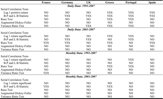
Table 6 summarizes the results of all the tests performed.

TABLE 6

Summary of Test Results: Random Walk Hypothesis Rejected?

France Germany UK Greece Portugal Spain

Daily Data: 1993-2007

Serial Correlation Tests

Lag 1 positive return NO NO NO YES YES YES

B-P and L-B Statistic NO YES YES YES YES YES

Runs Test NO NO NO YES YES NO

Augmented Dickey-Fuller NO NO NO NO NO NO

Variance Ratio Test NO NO YES YES YES NO

Daily Data: 2003-2007

Serial Correlation Tests

Lag 1 return significant NO NO NO YES YES NO

B-P and L-B Statistic NO YES YES NO YES NO

Runs Test YES YES NO YES NO YES

Augmented Dickey-Fuller NO NO NO NO NO NO

Variance Ratio Test NO NO NO NO NO NO

Monthly Data: 1993-2007

Serial Correlation Tests

Lag 1 return significant NO NO NO NO YES NO

B-P and L-B Statistic NO NO NO NO NO NO

Runs Test NO NO NO YES YES NO

Augmented Dickey-Fuller NO NO NO NO NO NO

Variance Ratio Test YES NO NO NO NO NO

Monthly Data: 2003-2007

Serial Correlation Tests

Lag 1 return significant NO NO NO NO NO NO

B-P and L-B Statistic YES NO NO YES NO NO

Runs Test NO NO NO NO NO NO

Apart from the ADF test, which is very clearly favorable to the random walk hypothesis,

all other tests provide mixed evidence. Positive serial correlation has been very strong in daily

returns, in the case of Greece and Portugal, but declining in the last five years. This evidence

of persistency in prices is consistent with the findings of: (i) fewer runs than were expected

and (ii) the variance ratios tend to grow with the time lag.

For France, Germany, UK and Spain, most of the evidence does not allow the rejection

of the null hypothesis, thus favoring the random walk interpretation. In the case of France, the

runs test fails due to an excessive number of runs in daily data and the variance ratio fails in

monthly data. Germany, UK and Spain meet all random walk criteria, in monthly data.

References

Abraham, A., Seyyed, F. and Alsakran, S. “Testing the Random Behavior and Efficiency of the Gulf

Stock Markets” The Financial Review, 37, 3, 2002, pp. 469-480.

Dias, J., Lopes, L., Martins, V. and Benzinho, J.. “Efficiency Tests in the Iberian Stock Markets”,

2002, Available at SSRN: http://ssrn.com/abstract=599926.

Fama, E. “Efficient Capital Markets: A Review of Theory and Empirical Work” Journal of Finance,

25, 2, 1970, pp. 283-417.

Fama, E. and French, K. “Permanent and Temporary Components of Stock Prices” Journal of

Political Economy, 96, 2, 1988, pp. 246-273.

Gama, P. “A Eficiência Fraca do Mercado de Acções Português: Evidência do Teste aos Rácio de

Variância, da Investigação de Regularidades de Calendário e da Simulação de Regras de

Transacção Mecânicas”, Revista de Mercados e Activos Financeiros, 1, 1, pp. 5-28.

Grieb, T. and Reyes, M. “Random Walk Tests for Latin American Equity Indexes and Individual

Groenewold, N. and Ariff, M. “The Effects of De-Regulation on Share Market Efficiency in the

Asia-Pacific”, International Economic Journal, 12, 4, 1999, pp. 23-47.

Huang, B. “Do Asian Stock Markets Follow Random Walks? Evidence from the Variance Ratio Test”,

Applied Financial Economics, 5, 4, pp. 251-256.

Liu, C. and He, J. “A Variance-Ratio Test of Random Walks in Foreign Exchange Rates”, Journal of

Finance, 46, 2, p. 773-785.

Lo, A. and MacKinlay, A. “Stock Market Prices do not Follow Random Walks: Evidence from a

Simple Specification Test”, The Review of Financial Studies, 1, 1, 1988, pp. 41-66.

Ma, S. and Barnes, M. “Are China’s Stock Markets Really Weak-form Efficient?”, Centre for

International Economic Studies, Adelaide University, Discussion Paper 0119, May 2001.

MacKinnon, J. “Approximate Asymptotic Distribution Functions for Unit-Root and Cointegration

Tests”, Journal of Business & Economic Statistics, 12, 2, 1994, pp. 167-176.

Magnusson, M. and Wydick, B. “How Efficient are Africa’s Emerging Stock Markets”, Journal of

Development Studies, 38, 4, 2002, pp. 141-156.

Panas, E. “The Behaviour of Athens Stock Prices”, Applied Economics, 22, 12, 1990, pp. 1715-1727.

Smith, G., Jefferis, K. and Ryoo, H. “African Stock Markets: Multiple Variance Ratio Tests of

Random Walks”, Applied Financial Economics, 12, 4, 2002, pp. 475-484.

Smith, G. and Ryoo, H. “Variance Ratio Tests of the Random Walk Hypothesis for European

Emerging Stock Markets”, The European Journal of Finance, 9, 3, 2003, pp. 290-300.

Urrutia, J. “Tests of Random Walk and Market Efficiency for Latin American Emerging Markets”,

Journal of Financial Research, 18, 3, 1995, pp. 299-309.

Wheeler, F., Neale, B., Kowalski, T. and Letza S. “The Efficiency of the Warsaw Stock Exchange

Stock Exchange: The First Few Years 1991-1996”, The Poznan University of Economics Review,

2, 2, 2002, pp. 37-56.

Worthington, A. and Higgs, H. “Random Walks and Market Efficiency in European Equity Markets”,