1
HOW DOES HOUSEHOLD ENERGY CONSUMPTION CONTRIBUTE TO PM10 EMISSIONS?
CATARINA PACHECO VARELA GUSMÃO | STUDENT N. 435
MASTER IN ECONOMICS | MAJOR IN PUBLIC POLICY ANALYSIS
A project under the supervision of:
PROFESSOR MARIA ANTONIETA CUNHA E SÁ
PROFESSOR SOFIA FRANCO
2
HOW DOES HOUSEHOLD ENERGY CONSUMPTION CONTRIBUTE TO PM10 EMISSIONS?
Abstract: Particle Pollution (PM) is a major problem in urban environments. There is serious health risks associated with exposure to PM. In addition, particulate matter also contributes to greenhouse effects and global warming. PM originates mainly from fuel combustion. In this paper, we attempt to study household energy use contributions to experienced levels of PM concentrations. We find that there is a strong positive association between household gasoline consumption and urban air pollution. Residential natural gas use is also associated with poor air quality.
3 1. INTRODUCTION
Air pollution is a major environmental problem. There are many air pollution sources with different impacts on human health. In particular, exposure to particulate matter (PM) and ozone (O3) entail serious health risks. The effects of PM on health
occur at levels of exposure currently being experienced by most urban and rural populations around the world. Mortality rates in cities with high levels of pollution exceed those observed in relatively cleaner cities by 15-20% (WHO, 2011). Yet, exposure to air pollutants is beyond individuals’ control. Pollution in cities significantly
degrades quality of life and threatens their ability to attract households, firms and visitors.
The largest source of air pollution in most cities is motor vehicles. Other important sources are industries, space cooling and heating and commercial activities.. Although the use of cleaner fuels and technology contributed to the reduction of emissions from individual motor vehicles, increases in the volume of traffic add to environmental stress in cities. «The world is undergoing the largest wave of urban growth in history» (UNFPA, 2007). Given the slow pace of pollution control measures, air quality will continue to deteriorate.
Roughly half of the world’s population lives in cities and this share is rapidly increasing. Moreover, city dwellers consume 80% of all commercial energy produced globally and account for about the same share of GHG emissions (UN-HABITAT, 2011). But cities also offer unique opportunities for energy efficiency improvements that reduce GHG emissions and contribute to climate change mitigation. Therefore, understanding the sources of air pollution in cities is paramount to design policies
4
towards greening urban consumption and production. Local actions have the potential to both improve cities’ environment and alleviate global environmental problems.
In Portugal, about 61% of total population in 2010 lived in cities, and this share is predicted to reach 71.4% by 2030 (UN-HABITAT, 2011). For the same year, the residential sector was responsible for about 16.1% of total energy consumption (BEN, 2010).
This study aims at examining how household’s energy use contributes to Portuguese cities air pollution. In particular, we consider three main sources of particulate matter: private within-city transportation (gasoline consumption); consumption of natural gas (heating and cooking); and consumption of electricity (heating, cooling, lighting and cooking) at the municipality level.
By using a two-stage estimation procedure, we first estimate the household demand of each energy use. We use the results obtained at the first-stage to estimate the contribution of households’ consumption patterns at the Portuguese municipality level on air pollution from PM.
Results of the study here reported show that a 1 unit increase in total annual gasoline consumption (tons of oil equivalent) is associated with 35.2% more air pollution. Likewise, residential natural gas consumption deteriorates air quality. Industrial areas add to air pollution, while green areas help to alleviate this problem.
The rest of this report is organized as follows: in Section 2 we provide a brief overview of literature relevant for this study. A description of data sources and variables is given in section 3. Section 4 presents the methodology used and in section 5 the main results are presented and discussed. Section 6 contains the main conclusions and recommendations.
5 2. LITERATURE REVIEW
Not much research was found analyzing the links between household energy consumption and air pollution. However, there are a few relevant studies that add a lot to our knowledge of the subject.
Kahn (2000) uses household-level information to study some of environmental consequences of suburbanization. Population dispersion leads to increases in household driving, home fuel consumption and land consumption. He documents the extra resource consumption associated with life in the suburbs. Results of this study show that suburbanites drive 31 percent more than their urban counterparts and consume more than twice as much land. The positive differential in resource consumption is not translated in local air quality degradation in sprawling areas, though this fact is not fully addressed in this paper. Still, there is evidence that technological innovation can mitigate some of the environmental consequences of suburbanization. In a subsequent study, Glaeser and Kahn (2010) attempt to quantify the carbon dioxide emissions associated with new construction in 66 major metropolitan areas within the United States. In each of these metropolitan areas they predict emissions from driving, public transit, home heating and household electricity usage for a standardized household. They also perform this comparison between central cities and suburbs. Carbon dioxide emissions differentials within metropolitan areas are smaller than these differences across metropolitan areas. High temperatures imply higher emissions resulting of an extra use of electricity for cooling. In addition, cities generally have significantly lower emissions than suburban areas. In a more recent study, the same procedure is applied in analyzing 74 major Chinese cities (Zheng et al, 2008) and similar results were obtained.
6 3. DATA SOURCES AND DESCRIPTION
The Portuguese territory is divided in several administrative units. The smallest administrative divisions are parishes. Parishes are then clustered in municipalities – which possess some decision-making independence – which are grouped in districts. There are 308 municipalities in Portugal, inhabited by about 10.5 million people (INE, 2011).
Portuguese cities generally include more than one parish. Municipalities can include more than one city. There are two metropolitan areas (MA) in Portugal, Lisbon Metropolitan Area (LMA) and Porto Metropolitan Area (PMA).
Fig. 1 Map of Portuguese mainland showing the 37 municipalities included in our sample. The five statistical regions (NUTS II) designated in the analysis are highlighted in the map. Municipalities where the two main coal power plants are located are also identified.
7
We analyze the contribution of household energy consumption and location-level specific characteristics on air pollution (PM10). The unit of analysis is the
municipality. Our study area is composed by 37 municipalities located in the Portuguese mainland, which are inhabited by approximately 4.2 million people, for the years 2004, 2005, 2006, 2007 and 2009. The map in Fig. 1 represents the region that is studied (mainland Portugal). Particulate matter (PM10) is the primary indicator of environment
air pollution. We consider three main sources of PM10: transport and residential fuel
energy consumption (electricity and natural gas).
3.1. Data Sources
Household Characteristics
Data on the characteristics of the municipalities was retrieved from the online database of the Portuguese statistical office, Instituto Nacional de Estatística (INE, 2011). Data on household consumption data per municipality was collected by the Portuguese delegation for Energy and Geology, Direcção Geral de Energia e Geologia (DGEG), for the years 2004-20091. Demographics of the population and dwelling characteristics were obtained from the Portuguese census (INE, 2001). Income is provided by the Ministry of Social Security, Ministério do Trabalho e Segurança Social (MTSS/GEP) for the years 2004-2009. The data from the Portuguese population census were obtained for the year 2001 and assumed to be constant for the whole period.
Air Pollution (PM10)
Data for PM10 was collected from an online database on air quality (QUALAR)
provided by the Portuguese Environmental Agency, Agência Portuguesa do Ambiente
1
8
(APA). There are 72 active stations all over Portugal, and other 23 stations recently deactivated. Information was collected for the years 2004-2009 from both active and deactivated stations prepared to monitor particulate matter emissions. QUALAR dataset reports annual average PM10 emissions for each monitoring station. Since some of these
stations are located in the same municipality and our unit of analysis is the municipality, we have computed the average of emissions for these stations.
Land Allocation
Information on the different uses of soil was made available by the Portuguese Delegation for Urban Development and Planning, Direcção Geral de Ordenamento do Território e Desenvolvimento Urbano (DGOTDU) and published online by INE (2011). Data is available for the years 2005-2008. It provides information on the total area allocated to industrial activities and green areas for each municipality, defined in mandatory Municipal Development Plans, Plano Municipal de Ordenamento de Território (PMOT). Data on industrial and green areas are published only for the years 2005 to 2008. Hence, we assumed that the values for the year 2004 are the same as in year 2005, and those for year 2009 are the same as year 2008. Data were also collected on the density of roads, defined as total km of roads over total municipality area (Km2), made available by the Portuguese Authority for Roads, Estradas de Portugal (EP, 2007) and retrieved online from INE’s database (2011). Since this information is only available for the year 2007, we assume roads’ density to be constant over that period.
Climate
Climate exposure for each municipality is obtained from the Portuguese Weather Office, Instituto de Meteorologia (IM), and published online from PORDATA database (2011). Collected information is on annual average temperature and annual total
9
precipitation for the years 2004-2009. IM database contains annual average temperature and total annual precipitation measurements for each station in the database. Across the Portuguese mainland, there are six weather stations (Porto, Viana do Castelo, Bragança, Castelo Branco, Lisboa and Faro). Each municipality was then assigned to one of these stations using a proximity criterion.
Descriptive statistics for the sample are shown in Table 1. Our final sample includes 37 municipalities in a 5 year-period.
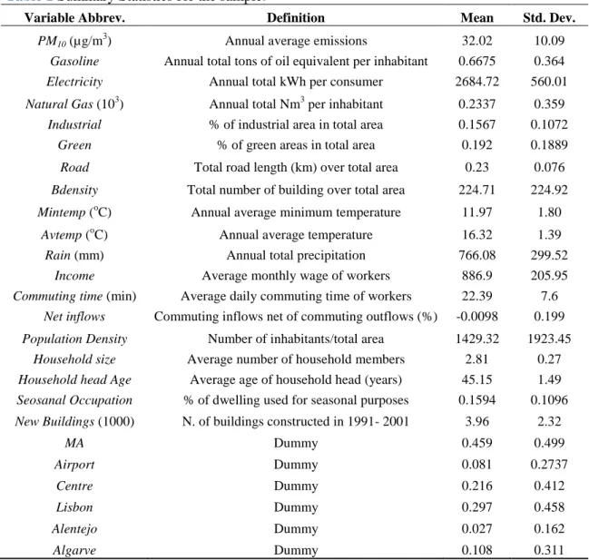
Table 1 Summary Statistics for the sample.
Variable Abbrev. Definition Mean Std. Dev.
PM10 (µg/m3) Annual average emissions 32.02 10.09
Gasoline Annual total tons of oil equivalent per inhabitant 0.6675 0.364
Electricity Annual total kWh per consumer 2684.72 560.01
Natural Gas (103) Annual total Nm3 per inhabitant 0.2337 0.359
Industrial % of industrial area in total area 0.1567 0.1072
Green % of green areas in total area 0.192 0.1889
Road Total road length (km) over total area 0.23 0.076
Bdensity Total number of building over total area 224.71 224.92
Mintemp (oC) Annual average minimum temperature 11.97 1.80
Avtemp (oC) Annual average temperature 16.32 1.39
Rain (mm) Annual total precipitation 766.08 299.52
Income Average monthly wage of workers 886.9 205.95
Commuting time (min) Average daily commuting time of workers 22.39 7.6
Net inflows Commuting inflows net of commuting outflows (%) -0.0098 0.199
Population Density Number of inhabitants/total area 1429.32 1923.45
Household size Average number of household members 2.81 0.27
Household head Age Average age of household head (years) 45.15 1.49
Seosanal Occupation % of dwelling used for seasonal purposes 0.1594 0.1096
New Buildings (1000) N. of buildings constructed in 1991- 2001 3.96 2.32
MA Dummy 0.459 0.499 Airport Dummy 0.081 0.2737 Centre Dummy 0.216 0.412 Lisbon Dummy 0.297 0.458 Alentejo Dummy 0.027 0.162 Algarve Dummy 0.108 0.311
10
Sampled municipalities present an annual 24-hour average particulate matter concentration of 32.2 micrograms per cubic meter of air (µg/m3), which is below the defined safe maximum threshold of 50 µg/m3 (APA, 2011. The representative household earns 886.9€/month and is composed by 2.81 members, which head is 45 years old. Annual average household gasoline consumption is 0.6675 toe. Residential electricity use per household is 2684.72 kWh/year and natural gas consumption is 0.2337 thousand Nm3/year.2
3.2 Variables Description
Household Characteristics and Energy use
Total household energy use is determined by a set of variables. These variables can be grouped in economic variables (household income and energy prices), demographic variables (household size, age of head, rural/urban location) and dwelling attributes (covered area of dwelling, age, construction type).
Gasoline use depends mainly on income and household characteristics, public transit availability and cities development patterns (Glaeser and Kahn, 2008). In Portugal, residential electricity is mainly used for lighting and heating/cooling, and its consumption is determined by both household and dwellings characteristics. In general new homes are associated with higher electricity consumption (Wiesmann et al., 2011).
Natural gas use in residencies is related to heating and cooking activities. Except for lighting purposes, natural gas and electricity can be considered alternative energy sources. Yet, the supply of natural gas in Portugal is not universal and not all municipalities have access to this type of energy. Still, natural gas yields lower levels of
2 Normal cubic meter
11
air pollution when compared to the other fuels used to produce electricity (fuel oil and coal).
Prices of energy were not introduced in the analysis. Both electricity and natural gas prices are regulated in Portugal, namely, for domestic use. Although consumers are already free to choose their provider, prices charged are fairly the same. The same happens with gasoline prices, which are virtually the same across the country.
Air Pollution (PM10)
Particle pollution impact negatively on human health and it’s acknowledged to be the cause of increased prevalence of respiratory diseases (APA, 2011). Particulate matter (PM) is a mixture of extremely small particles and liquid droplets. PM is generally categorized on the basis of the size of the particles, which is directly linked to their potential for causing health problems. Primary particles are emitted directly from sources like paved and unpaved roads, construction, fields and fires. Secondary particles originate from reactions in the atmosphere originated in chemicals emitted by power plants, industries and automobiles (EPA, 2011).
Energy Use and Air Pollution
Transportation is the main source of air pollution in cities (EPA, 2011). Both gasoline consumption and corresponding generated pollution depend on several factors. While electricity is consumed differently across locations, its production takes place in specifically located power plants across the Portuguese territory. Hence, production and consumption points are separated and it is expected that areas where these power plants are located concentrate most of pollution associated with electricity consumption.
12
Generally, power plants are located outside urban areas. The two most pollutant thermoelectric coal power plants are located in Sines municipality ( Central de Sines in Alentejo region) and in Abrantes municipality (Central do Pego in Lisbon region) (REN, 2011). Fig. 1showsthe location of all thermoelectric power plants.
Cities and Air Pollution
Energy use is not the only determinant of air pollution of a city environment. Cities building patterns determine how pollution spreads across space. A very dense construction pattern contributes to wind decelerations and higher temperatures in city centers (microclimate) that aggravate air pollution consequences. Also, different city infrastructure and climate exposure influence life-styles and energy uses. Temperatures, precipitation and wind flows influence both air pollution levels and consumption (cooling/heating). Green areas, in contrast, have pollutant absorptive capacity and contribute to cooling of urban environments.
3.3. Remarks about dataset
Data presents some quality heterogeneity. Information on both gasoline and natural gas consumption doesn’t present the same quality as data on electricity
consumption. A second issue regards the absence of data residential natural gas consumption at a municipality level. Most likely, it also includes natural gas use for industrial purposes. The use natural gas for industrial activities generates higher levels of air pollution than when it is used in residencies. So, the ―true‖ relationship between residential natural gas use and pollution may be overstated.
Another important point to make is that particulate matter measurement stations are located in specific places in each municipality and capture solely emissions concentrated in a given perimeter.
13 4. METHODOLOGY
We use a two-stage least-square estimation procedure to estimate the contribution of household demand for energy consumption on air pollution (PM10). In a first step, we estimate household energy consumption across municipalities. In a second step, the results obtained in the first-step are used to relate household consumption to particle pollution.
4.1 Energy Use
Household energy use per municipality is considered as a derived demand. In standard economic theory, individuals are assumed to choose their optimal consumption by maximizing utility subject to their budgetary constraints. Despite that we are not estimating individual energy demands, we assume that aggregated demand at a municipality level depends on the same arguments as individual demands.
Thus, the derived demand for individual energy use can be represented by equation (1), as follows:
(1)
where gasoline, electricity and natural gas use in municipality , is a vector of household characteristics in municipality ,
reflects the impact of those variables, is an error term. refers to price of energy
, refers to household income, refers to a vector of household characteristics, refers to a vector of dwellings attributes and refers to a vector of geographic location
14
The dependent variable in (1) is presented in levels, except for electricity consumption which is presented in logarithmic form
4.2. Air Pollution (PM10)
The second-stage uses energy demands estimated in (1) as explanatory variables of particulate matter concentrations, as follows:
(2)
where stands for gasoline, electricity and natural gas use in municipality , refers
to the value of local characteristic in municipality , reflects the impact of those variables and is a municipality level error term.
The sample consists of 185 observations. We use ordinary least squares (OLS) to estimate all the models’ coefficients. In (2) the dependent variable is the natural
logarithm of particulate matter with a diameter equal or less than 10 micrometers. However, not all explanatory variables are presented as natural logarithms.
Several functional forms were considered in order to choose each model’s best fit. We only show the results for the best fit models, that is, presenting the highest R-squared. The variance inflation factor (VIF), condition index, tolerance, and the covariance and correlation matrices were used to assess multicollinearity among the independent variables in the model. Since in our model VIF was less than 9 for all variables, multicollinearity between the independent variables is not a problem.
Annual dummies for the 5-year period are introduced in (2). The reference category is the year 2004. These variables are not used in (1) because our purpose in the first-step is to estimate annual demands for each type of energy. In (2) we also included
15
a dummy variable for the level of urbanization and the presence of an airport, as well as dummy variables to account for the different regions. The categories for the dummy variable for the level of urbanization are no metropolitan area (reference category) and metropolitan area. The regions we controlled for were North (reference category), Center, Lisbon, Alentejo and Algarve. The five regions are identified inFig. 1.
5. ESTIMATION RESULTS
5.1. Demand for Energy
The results for the estimation of equation (1) are shown in Table 2, Table 3and
Table 4 for the three types of energy use.
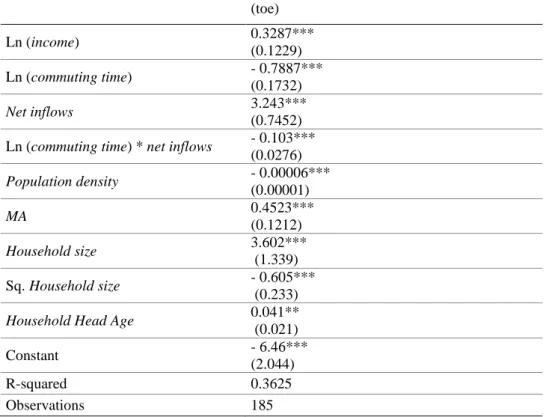
Gasoline Use
Table 2 presents estimates for gasoline consumption per municipality. This variable is regressed on household-level characteristics and local fixed effects. The overall R2 is 36.25%. Family size, household head age, and income strongly increase gasoline consumption, so it is important to control for these characteristics. Remind that all Portuguese households face the about the same price of gasoline and thus, this variable is not introduced in the analysis. The estimated income elasticity for gasoline consumption is 0.49, meaning that one percent increase in income leads to a 0.49% increase in gasoline consumption.
The area-level characteristics have the expected signs. Population density reduces gasoline usage. This variable is an indicator of how suburban is the area where the household lives. The higher the population density, then, all else equal, household driving should be lower. On average, a 1000 unit increase in population density is
16
associated with a 0.06 toe reduction in total annual gasoline consumption (-.12 the corresponding elasticity). Metropolitan areas residents consume, on average, 0.4523 more toe in gasoline per year when compared with people living outside MAs. The coefficients on the variables related to commuting patterns are highly statistically significant. The positive coefficient on net commuting inflows suggests the impact of car dependency for commuting purposes. In contrast, commuting time presents a negative coefficient.
Table 2 Tons of oil equivalent consumed per year
Per capita total annual gasoline consumption (toe) Ln (income) 0.3287*** (0.1229) Ln (commuting time) - 0.7887*** (0.1732) Net inflows 3.243*** (0.7452) Ln (commuting time) * net inflows - 0.103***
(0.0276) Population density - 0.00006*** (0.00001) MA 0.4523*** (0.1212) Household size 3.602*** (1.339) Sq. Household size - 0.605*** (0.233)
Household Head Age 0.041**
(0.021)
Constant - 6.46***
(2.044)
R-squared 0.3625
Observations 185
***, ** and * indicates statistical significance at the 1%, 5% and 10% level, respectively. Robust standard errors in parentheses
17
Electricity Consumption
Table 3 presents the estimates for municipality’s log of annual per-consumer electricity
consumption explained by household characteristics and both local and regional fixed effects.
Table 3 kWh of electricity consumed per year.
Natural logarithm of total annual electricity consumption per consumer (kWh)
Ln (income) 0.205*** (0.051) Household size 2.454*** (0.661) Sq. Household size -0.459*** (0.113)
Household Head Age -0.053***
(0.014) Centre -0.189*** (0.027) Lisbon -0.376*** (0.037) Alentejo -0.160** (0.069) Algarve -0.2592*** (0.053) Ln (seasonal occupation) -0.118*** (0.019) Mintemp 0.017** (0.008) Ln (new building) 0.045* (0.027) Constant 5.32*** (1.49) R-quared 0.7651 Observations 185
***, ** and * indicates statistical significance at the 1%, 5% and 10% level, respectively. Robust standard errors in parentheses
This model has a good fit, presenting an overall R2 of 76.51%. Electricity consumption is an increasing function of income – income elasticity is 0.205 – and household size. Families with more members consume less electricity per member. One year increase in the age of the household head leads to a 5% decrease in electricity consumption, on average. Seasonal use of dwelling, as expected, decreases total annual
18
electricity consumption. The number of houses built between the years 1991-2001 increases electricity consumption, in accordance with we have discussed before. In addition, electricity use increases 1.7% for one Celsius degree increase in annual average temperature, other things equal.
Natural Gas Consumption
Table 4 presents the results for natural gas consumption. The number of observations used is limited to the municipalities where natural gas is supplied. Natural gas use is also positively related to income and household size. Yet, income elasticity for natural gas is 3.32. Natural gas can be considered a superior good associated to high levels of income.
Table 4 Nm3 of natural gas consumed per year.
Per capita total annual natural gas consumption (Nm3 millions)
ln (income) 0.7759***
(0.192) ln (household size) 6.711***
(0.860)
Household Head Age 0.271***
(0.040) Centre 0.767*** (0.108) Lisbon 0.030 (0.072) Algarve 0.519*** (0.116) ln (new building) 0.127*** (0.039) Seasonal use -1.121*** (0.287) Mintemp 0.150*** (0.025) Constant -26.147*** (3.66) R-quared 0.6380 Observations 146
***, ** and * indicates statistical significance at the 1%, 5% and 10% level, respectively. Robust standard errors in parentheses
19
New housing has a positive impact on natural gas consumption. Again, this is related to the fact that, in general, new buildings demand more space and dwellings are bigger. Also, new housing infrastructures are more likely to be prepared to support natural gas supply, while older buildings don’t. The coefficient of minimum
temperature is significant at a 1% significance level, which was not expected if we assume that natural gas is also used for residential heating. The ICESD survey (2010) relates natural gas consumption to be only 9.3% of total energy consumption, while electricity accounts for about 43% of total consumption. Moreover, natural gas use in residencies is reported to be mainly for hot water (61.8%) and cooking (35.1%), while its use for heating is minimal (3.1%).
5.2. Particulate matter emissions
Table 5 presents six regression estimates for the particulate matter equation presented in equation (2).
Specification #6 includes all relevant variables that we have discussed in previous sections. It presents the highest overall R2, of about 65%. Across the three types of energy use, only gasoline and natural gas are statistically significant. These results are as expected since gasoline consumption is considered to be one of the main sources of PM10. Regarding natural gas, these results may be related to industrial uses.
The fact that electricity consumption is not significant reflects that the contribution of electricity use to PM10 concentrations is related to production, but we did not control for
the local existence of power plants.
A 1 unit increase in total annual toe of gasoline consumed is now associated with an increase of 35.2% in air pollution, ceteris paribus. For natural gas
20
consumption, total annual Nm3 unitary changes lead to an increase of 26.9% in pollution levels. For small green areas the impact on pollution is negative, and statistically significant. Yet, as these areas get bigger, the overall contribution to pollution becomes positive. Thus, both the specific location and the dimension of green areas influence the way they contribute to pollution absorption in a city environment. All coefficients on regional dummies are statistically significant and these are positive for all regions, except for the center region. When compared to the North, Southern regions are associated with larger pollution levels on average. Climate effects are probably causing this relationship, as southern locations are exposed to hot summers, which we have shown contribute to an increase in electricity usage.
Total precipitation was higher in the years 2007 and 2009, determining the use of clean energies to produce electricity and explaining the statistical significance of these years in the regression. Moreover, total precipitation contributes to a decrease of PM10 concentrations in the air. The coefficient on Lisbon Metropolitan Area (LMA) is
negative and statistically significant. Metropolitan areas have more driving, but they are also more likely to have extensive public transit systems that alleviate pollution problems (Glaeser and Kahn, 2008).
When analyzing the different specifications, one can have a better idea on how these variables interact in explaining particulate matter pollution. Specification #1 includes only municipalities’ fixed effects and household energy consumptions. Energy
use variations alone explain about 20% of all the variations in particulate matter emissions. Yet, only the coefficient on electricity consumption is statistically significant. In specification #2, variables on specific uses of land, economic activities and building patterns are introduced in the regression, increasing the quality of the
21
model. Industrial areas reveal a highly significant negative impact on air pollution. This relationship is almost for sure spurious and might be related to specific location choices of industries outside urban areas, where emissions monitoring stations are scarcer. In what concerns cities development patterns, denser cities are, on average, associated with more air pollution, with an elasticity of 0.112.
Specification #3 includes a dummy variable for the existence of an airport as explanatory variable. The introduction of such a variable lowers the overall quality of the model. Therefore, the following specifications will not include it. It might be surprising that this variable doesn’t add to explain PM10 concentrations. Yet, pollution
originating from airports might either not be related with particulate matter concentrations or the result may be related with the location of the monitoring stations.
When we run an additional regression with local weather exposure variables, in specification #4, it is observed that total precipitation impacts negatively on air pollution. A 1% variation on total annual precipitation is associated with a 0.22% decrease in air pollution levels. When regional dummies are introduced in the regression, these coefficients are no longer statistically significant.
Introducing region fixed effects and annual dummies changes dramatically the results and improves the fit of the model. In specification #5 only regional and MA dummies are introduced in the regression. The coefficient on electricity consumption is no longer statistically significant and instead, both gasoline and natural gas consumption increase total emissions significantly. Both Centre and Alentejo regions effects are significantly related to air pollution.
22 Table 5 Average Annual PM10 Emissions
Ln (PM10) Specification 1 2 3 4 5 6 0.090 (0.093) 0.100 (0.109) 0.112 (0.111) 0.038 (0.110) 0.283** (0.129) 0.352*** (0.109) 0.748*** (0.117) 0.412** (0.169) 0.428** (0.171) 0.733*** (0.198) -0.033 (0.261) -0.116 (0.236) 0.030 (0.079) 0.033 (0.083) 0.024 (0.088) 0.163* (0.088) 0.268*** (0.089) 0.269*** (0.075) Green 0.541 (0.435) 0.656 (0.462) 0.549 (0.426) -0.664 (0.415) -0.891** (0.352) Sq. Green -0.477 (0.629) -0.599 (0.649) -0.689 (0.590) 0.635 (0.556) 0.899* (0.459) Industrial 2.633*** (0.766) 2.569*** (0.775) 1.497** (0.734) 2.976*** (0.900) 3.064*** (0.776) Sq. Industrial -5.799*** (1.479) -5.716*** (1.490) -3.544** (1.439) -4.926*** (1.727) -4.920*** (1.420) Ln (Road) -0.117 (0.093) -0.111 (0.093) -0.050 (0.093) -0.149 (0.126) -0.135 (0.118) Ln (Bdensity) 0.112*** (0.029) 0.108*** (0.093) 0.099*** (0.028) 0.306*** (0.054) 0.323*** (0.050) Airport -0.071 (0.077) Ln (Avtemp) 0.504 (0.316) -0.094 (0.504) -0.142 (0.491) Ln (rain) -0.220*** (0.062) -0.208*** (0.062) 0.061 (0.142) MA* Lisbon -0.649*** (0.206) -0.701*** (0.189) MA* Porto -0.139* (0.083) -0.120 (0.073) Centre -0.328*** (0.125) -0.243* (0.125) Lisbon 0.354 (0.229) 0.506** (0.220) Alentejo 0.391** (0.194) 0.534*** (0.189) Algarve 0.165 (0.234) 0.430* (0.235) Year 2005 0.017 (0.062) Year 2006 -0.136 (0.089) Year 2007 -0.141** (0.054) Year 2009 -0.353*** (0.081) Constant -2.549*** (0.914) -0.910 (1.320) -1.014 (1.339) -3.110 (2.060) 3.270 (2.052) 2.220 (2.191) R squared 0.2042 0.4089 0.4113 0.4518 0.5585 0.6499 Root MSE 0.31123 0.2728 0.27302 0.26423 0.24135 0.21752 Observations 185 185 185 185 185 185
***, ** and * indicates statistical significance at the 1%, 5% and 10% level, respectively. Robust standard errors in parentheses
23 6. CONCLUSION
This study has documented that, controlling for local-specific characteristics, private gasoline consumption and residential natural gas consumption contribute to local air pollution, namely particle pollution, in Portuguese municipalities. We also find significant evidence that specific urban features also determine particle pollution. Building density, green areas and industries affect consumption patterns and local air quality.
Based on these results, urban policies should be designed towards both the reduction of car dependency and technological improvements in the existing vehicle fleet. Vehicle emissions control measures reduce the impact of individual cars, if they can compensate for increasing traffic levels. Reduction of car usage in cities depends greatly on alternative transportation options. Redesigning and reinforcing current models of public transport are possible solutions. Another and complementary option is to set independent cycle tracks that induce the use of environmental-friendly transportation modes.
Here, we also verify that green areas have positive impacts on air quality. Thus, current land development plans, from which we collect information on green areas, are already ―enjoying‖ the benefits of their absorptive capacity. Still, there is a great
potential to be exploited. Allocating green areas to urban settings should be a major concern when trying to manage growing urbanization and air pollution levels. Moreover, construction patterns that comply with local climates and alleviate pollutants concentration in urban atmospheres should be preserved and/or promoted.
This paper has some limitations. The main problem is related with data availability and heterogeneity. The sample in use may not be representative of the
24
Portuguese population. Thus, we base our conclusions on regressions that can provide only an imperfect estimate of particle pollution. Future research should attempt to use a smaller unit of analysis – a parish, for example – covering a wider area of the country, and expand the analysis to other household polluting sources.
REFERENCES
[1]Auffhammer, M., Bento, A., and Lowe S. E.,2009. Measuring the effects of the Clean Air Act Amendments on ambient PM10 concentrations: The critical importance of a spatially disaggregated analysis. Journal of Environmental Economics and Management, vol. 58 (1), 15–26.
[2]Dergiades, T. & Tsoulfidis, L. (2008), Estimating Residential Demand for Electricity in the United States, 1965-2006, Energy Policy, Vol. 30, 2722-2730.
[3]DGEG, 2011. Estatísticas e Preços – Balanços e Indicadores Energéticos, Balanço Energético Nacional 2010 (provisório), Direcção Geral de Energia e Geologia. Retrieved from http://www.dgge.pt/.
[4]DGEG, 2011. Estatísticas e Preços – Balanços e Indicadores Energéticos, ICESD – Inquérito ao Consumo de Energia no Sector Doméstico (relatório final), Direcção Geral de Energia e Geologia. Retrieved from http://www.dgge.pt/
[5] EPA, 2011. Air & Radiation – Particulate Matter. U.S. Environmental Protection Agency. Retrieved from http://www.epa.gov/air/particlepollution/.
[6] Glaeser, Edward L. & Kahn, Matthew E., 2010. "The greenness of cities: Carbon dioxide emissions and urban development," Journal of Urban Economics, Elsevier, vol. 67(3), 404-418.
[7]INE, 2003. Censos—Antecedentes, metodologias e conceitos—2001. Instituto Nacional de Estatística, Portugal. Retrieved from http://www.ine.pt.
[8] Kahn, M. E., 2000. The environmental impact of suburbanization. Journal of Policy Analysis and Management, 19: 569–586.
25
[9] Zheng, S., Wang, R., Kahn, M.E., Glaeser, E.L., 2008. The Greenness of China: Household Carbon Dioxide Emissions and Urban Development. Journal of Economic Geography, vol. 11(5), 761-792(32).
[10] UNFPA, 2007. State of World Population 2007: Unleashing the Potential of Urban Growth. Retrieved from http://www.unfpa.org/swp/swpmain.htm
[11] UN-HABITAT, 2011. E-Resources – Urban Indicators. The United Nations Human Settlements Programme. Retrieved from
http://www.unhabitat.org/stats/Default.aspx.
[12] Wiesmann, D., Azevedo, I.L., Ferrão, P., Fernández, J., 2011. Residential electricity consumption in Portugal: Findings from top-down and bottom-up models. Energy Policy, 39, 2772-2779.
[13]Wu, Z., Hu, M., Lin, P., Liu, S., Wehner, B., and Wiedensohler, A., 2008. Particle number size distribution in the urban atmosphere of Beijing, China, Atmospheric Environonment, 42, 34, 7967–7980.