BioTextRetriever: a tool to Retrieve Relevant
Papers
Célia Talma Gonçalves
LIACC & Faculdade de Engenharia da Universidade do Porto &
Instituto Superior de Contabilidade e Administração do Porto & CEISE-STI, Portugal
Rui Camacho
LIAAD & DEI & Faculdade de Engenharia da Universidade do Porto, Portugal
Eugénio Oliveira
LIACC & DEI & Faculdade de Engenharia da Universidade do Porto, Portugal
ABSTRACT
Whenever new sequences of DNA or proteins have been decoded it is almost compulsory to look at similar sequences and papers describing those sequences in order to both collect relevant information concerning the function and activity of the new sequences and/or know what is known already about similar sequences that might be useful in the explanation of the function or activity of the newly discovered ones.
In current web sites and data bases of sequences there are, usually, a set of curated paper references linked to each sequence. Those links are very useful since the papers describe useful information concerning the sequences. They are, therefore, a good starting point to look for relevant information related to a set of sequences. One way is to implement such approach is to do a blast with the new decoded sequences, and collect similar sequences. Then one looks at the papers linked with the similar sequences. Most often the number of retrieved papers is small and one has to search large data bases for relevant papers.
In this paper we propose a process of generating a classifier based on the initially set of relevant papers. First we collect similar sequences using an alignment algorithm like Blast. We then use the enlarges set of papers to construct a classifier. Finally we use that classifier to automatically enlarge the set of relevant papers by searching the MEDLINE using the automatically constructed classifier. We have empirically evaluated our proposal and report very promising results.
Keywords: MEDLINE, Classification, Information Retrieval System, Machine Learning,
Ensemble Algorithms, Bioinformatics INTRODUCTION
Molecular Biology and Biomedicine scientific publications are available (at least the abstracts) in Medical Literature Analysis and Retrieval System On-line (MEDLINE). MEDLINE is the U.S. National Library of Medicine (NLM), premier bibliographic database: contains over 16 million
references to journal articles in life sciences with a concentration on Biomedicine. A distinctive feature of MEDLINE is that the records are indexed with NLM’s Medical Subject Headings (MeSH terms). MEDLINE is the major component of PubMed (Wheeler et al., 2006), a database of citations of the NLM. PubMed comprises more than 19 million citations for biomedical articles from MEDLINE and life science journals. The PubMed database maintained by the National Center for Biotechnology Information (NCBI) is a key resource for biomedical science, and is our first base of work. The NCBIs PubMed system is a widely used method for accessing MEDLINE.
The result of a MEDLINE/PubMed search is a list of citations (including authors, title, journal name, paper abstract, keywords and MeSH terms) to journal articles. The result of such search is, quite often, a huge amount of documents, making it very hard for researchers to efficiently reach the most relevant documents. As this is a very relevant and actual topic of investigation we assess the use of Machine Learning-based text classification techniques to help in the identification of a reasonable amount of relevant documents in MEDLINE. The core of the reported work is to study the best way to construct the data sets and the classifiers from the starting set of sequences.
These experiences were done using a set of positive examples associated to the sequences/keywords given by the user and a set of negative examples which is the focuses of this paper. The negative examples were generated in three different ways and we intend to show which is the best approach for our classification purpose. In our experiments we have used several classification algorithms available in the WEKA (Hall et al., 2009) tool including ensemble algorithms. We have also made some sensitivity tests to the pruning of attributes for attribute reduction.
The rest of the paper is structured as follows. The section “An Architecture for an Information Retrieval System” presents the architecture for our information retrieval system and the following Section “The Local Data base” describes the local data base construction process and the pre-processing techniques used. Follows the related work and a section dedicated to the “Automatic Construction of data sets” that describes the different alternatives proposed to data set construction and the experiences we have done with different classifiers. We also include a section dedicated to classifier ensemble where we present our experiments using classifier ensemble methods and finally we conclude the paper.
AN ARCHITECTURE FOR AN INFORMATION RETRIEVAL SYSTEM
The overall goal of our work is to implement a web based search tool that receives a set of genomic or proteomic sequences and returns an ordered set of papers relevant to the study of such sequences. The initial set of sequences is supplied by a biologist together with a set of relevant keywords and an e-value1. These three items are the input for BioTextRetriever
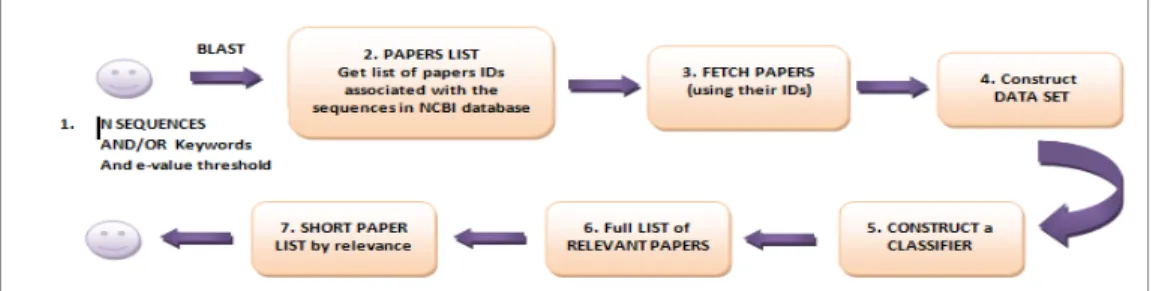
(Gonçalves & Camacho and Oliveira, 2011) as can be seen in Figure 1. Figure 1 presents a summary of our approach that we will now describe in detail. In the following description we use NCBI as the sequence Data Base.
Figure 1. Sequence of steps executed by BioTextRetriever when the user provides a set of initial DNA/protein sequences.
In Step 1, the user (a biologist researcher) provides an initial of sequences, optionally a list of keywords, and an e-value. With these three items (sequences, keywords and e-value) and using the NCBI BLAST tool we collect a set of similar sequences together with the paper references associated to them. We could also use Ensembl with the same inputs because Ensembl may return a different set of papers references. However for the proposed work we have only used the NCBI database.
With this list of paper citations we search for their abstracts in a local copy of MEDLINE (LDB – Local Database) (Step 3). For this we have previously preprocessed MEDLINE. Step 3 searches and collects the following information in the pre-processed local copy of MEDLINE: pmid, journal title, journal ISSN, article title, abstract, list of authors, list of keywords, list of MeSH terms and publication date.
For the scope of this paper we are considering only the paper citations that have the abstract available in MEDLINE. After Step 3 we have a data set of papers related to the sequences. We will take this set of papers as the positive examples for the full construction of the data set (Step 4) but we need to get some negative examples. To obtain the negative examples we have three possible approaches.
Thus this step is explained in detail in Section III.
The following step, Step 5, is one of the most important steps of our work which is to Construct a Classifier using Machine Learning techniques that is explained in the next section. As a result of this step we have a full list of articles considered relevant by our classifier (Step 6). However, we need to present them to the biologist in an ordered fashion way. So Step 7 presents an ordered list of relevant articles to
the biologist. Here we will develop and implement a ranking algorithm based on features such as the number of citations of the paper and the impact factor of the journal/conference where it was published. This paper focuses on the construction of the data sets highlighting the research from the different approaches to obtain the negative examples. According to the figure and for the purpose of this paper we focus on Step 4, although we have made a set of experiences with some classifiers to conclude what was the best approach.
THE LOCAL DATA BASE
We have downloaded 80GB (617 XML files) of MEDLINE 2010 from the NCBI website. Each XML file has information characterizing one citation. Among these characteristics we have considered the following ones: PMID - the PubMed Identifier; the PubMed Date; the Journal Title; the Journal ISSN that corresponds to the ISI Web of Knowledge ISSN; the Title; the
Abstract of the article if available; the list of the Authors; the MeSH Headings list and the Keywords list. After download the files were preprocessed as follows.
Pre-Processing MEDLINE XML files
An independent step of our tool is to maintain a local copy of MEDLINE, that we will call Local Data Base (LDB). The LDB will enable efficient search of the paper and will have that relevant information of each paper in format adequate, the algorithm that construct a chain as describe further in this paper.
The first step is to read the XML files and extract the relevant information to store in the LDB. Article’s title and abstract are preprocessed with “traditional” text pre-processing techniques. Next section presents the preprocessing techniques applied.
Pre-Processing Techniques
We have empirically (Gonçalves & Gonçalves & Camacho & Oliveira, 2010) evaluate which are the best combination of pre-processing techniques to achieve a better accuracy. Based on this previous study and with some more research in the meanwhile we have used the following preprocessing techniques.
Document Representation
For each paper with the information referred in the beginning of this section However the text facts of a document (title and abstract) are filtered using text processing techniques and represented using the vector space model from Information Retrieval where the value of a term in a document is given by the standard term-frequency inverse document frequency
(TFIDF=TF*IDF) function (Zhou & Smalheiser & Yu, 2006), to assign weights to each term in the document.
TF is the frequency of term in document and 1 sin log + = hterm cumentswit numberofdo collection cument numberofdo IDF
Named Entity Recognition (NER)
NER is the task of identifying terms that mention a known entity. We have used ABNER (Settles, 2005), which stands for A Biomedical Named Entity Recognition, that is a software tool for molecular biology that identifies entities in the biology domain: proteins, RNA, DNA, cell type and cell line. Although we have implemented this technique we have concluded that the identification of NER terms augments significantly the number of attributes instead of reducing them. We concluded that the use of NER increases strongly the number of terms which is a problem for the classifiers. Thus we did not use NER in the pre-processing phase.
Handling Synonyms
We handle synonyms using the WordNet (Fellbaum, 1998) to search for similar terms, in the case of regular terms, and used Gene Ontology (Ashburner, 2000) to find biological synonyms. If two words mean the same then they are synonyms, so they could be replaced by one of them in
the entire MEDLINE (title and abstract fields) without changing the semantic meaning of the term thus reducing the number of attributes. In this step we have replaced all the synonyms found by one synonym term thus reducing the number of terms.
Dictionary Validation
A term is considered a valid term if it appears in available dictionaries. We have gathered several dictionaries for the common English terms ( such as Ispell and WordNet) and for the medical and biological terms (BioLexicon (Rebholz-Schuhmann et al., 2008), The Hosford Medical Terms Dictionary (Hosford, 2004) and Gene Ontology (Ashburner, 2000). The Hosford Medical Terms Dictionary consists of a file that contains a long list of medical terms. BioLexicon is a large-scale terminological resource developed to address text mining requirements in the biomedical domain. The BioLexicon is publicly available both as an XML-formatted term repository and as a relational database (MySQL) and it adheres to the LMF ISO standards for lexical resources. We have also used the Gene Ontology available files that are related to genes, enzymes, chemical resources, species and proteins. We have processed each of these resource files in order to have a simple text file with one term per line.
Our approach is in the sense that if a term appears in one of these dictionaries it is a valid term, otherwise, it is not a valid term, so we remove it from the collection of terms.
The application of these technique is fundamental in attribute reduction once a lot of terms that have no biology, medical and normal significance are discarded.
Stop Words Removal
Stop Words Removal removes words that are meaningless such as articles, conjunction and prepositions (e.g., a, the, at, etc.). These words are meaningless for the evaluation of the document content. We have used a set of 659 stop words file.
Tokenization
Tokenization is the process of breaking a text into tokens. A token is a non empty sequence of characters, excluding spaces and punctuation.
Special Characters Removal
Special character removal removes all the special characters (+, -, !, ?, ., ,, ;, :, f, g, =, &, #, %, $, [, ], /, <, >, n, “, ”, j) and digits.
Stemming
Stemming is the process of removing inflectional affixes of words reducing the words to their stem (the words computer, computing and computation are all transformed into comput, which means that three different terms are transformed into only one term thus reducing the number of attributes. We implemented the Porter’s Stemmer Algorithm (Porter, 1997).
Pruning
Using pruning we discard in the documents collection terms that either appear too rarely or too frequently.
RELATED WORK
There are some work being done on biological and biomedical document classification. Some of them applied to MEDLINE document classification and other databases.
The work of (Sehgal, 2011) tries to automate the process of adding new information to TCDB database (Transport Classification Database) that is a web free access database (http://www.tcdb.org) about comprehensive information on transport proteins. The authors restricted themselves to the
documents in MEDLINE. The main goal is to highlight the use of Machine Learning techniques outperforms rules created by hand by a human expert. To train the classifier they have used a set of MEDLINE documents referred TCDB as positive examples and have selected randomly also from MEDLINE a set of negative examples.
The authors in (Imambi & Sudha, 2011) describe a new model for text classification using estimating term weights which improves accuracy classification according to the authors experiences. Documents are represented as vectors of terms with their normalized global frequency. Global weights are functions that count how many times a term appears in the entire collection and the normalization process compensates the discrepancies in the lengths of the documents. They have
used 1000 documents from PubMed; 600 documents for the training data set and 400 for the test data set. All these documents belong to four categories with MeSH terms related to Diabetes melitus. The authors compare the different weighting methods: local-binary, local-log, local df and global relevant. They concluded in this study that global relevant weighting method achieves a higher precision. In our own work we have also used all normalized global frequency.
BioQSpace (Divoli et al., 2005) is a GUI where users can query abstracts from PubMed using an embedded search facility. BioQSpace performs pairwise similarity calculations between all the abstracts based on a set of individual attributes namely: structure, function, disease and therapeutic compounds word list obtained from MeSH terms, word usage, PubMed related articles, publication date among others. These attributes are given more or less importance according to the weight attributed by users. A clustering algorithm is used to group abstracts that are very similar.
(Frunza & Inkpen & Tran, 2011) describe a methodology to build an application capable of identifying and disseminating health care information using a Machine Learning approach. The main objective of their work is to study the best information representation model and what classification algorithms are suitable for classifying relevant medical information in short texts. They have used 6 different Machine Learning algorithms. The authors concluded that naive Bayes performed very well on short texts in the medical domain and that adaboost had the worst result.
In (Dollah & Seddiqui & Aono, 2010) the authors present an approach for classifying a collection of biomedical abstracts downloaded from MEDLINE database with the help of ontology alignment. Although this work classifies MEDLINE documents it is based on ontology alignment which is out of our scope.
LigerCat (Sarkar et al., 2009) stands for Literature and Genomic Electronic Resource Catalogue, and it is a system for exploring biomedical literature through the selection of terms within a MeSH cloud that is generated based on an initial query using journal, article, or gene data. The central idea of LigerCat is to create a tag cloud showing an overview of important concepts and trends associated to the MeSH descriptors. LigerCat aggregates multiple articles in PubMed, combining
the associated MeSH descriptors into a cloud, weighted by frequency. LigerCat does not apply any Machine Learning techniques for paper classification as we present in our study.
AUTOMATIC CONSTRUCTION OF DATA SETS Constructing the Data Sets
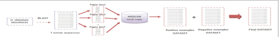
In order to solve our problem that is given a set of genomic or proteomic sequences return a set of related sequences and papers with relevant information for the study of such sequences, we need to obtain first of all the articles associated with the given set of sequences and construct the data set to give to the classifier. Figure 2 illustrates sequence of steps included in BioTextRetriver. The empirical work repeated in the paper concerns the construction of a data set (Step 4).
Figure 2. Data Set Construction
The input of our work is a set of sequences given in the FASTA format. We use the netblast-2.2.22 tool that perform a remote blast search at the NCBI site. We have embedded this application into our code and automatically have access to both, the original sequences and the set of similar sequences retrieved by BLAST.
These results show us the similar sequences and the evalue associated with each of the retrieved sequence. The e-value is a statistic to estimate the significance of a match between two sequences. The e-value is an input that is given us by the biologist. We relax this threshold value in order to obtain the negative examples based on the e-value as we can see in Figure 3. The positive examples are the one’s that are lower than the e-value previously specified by the biologist. We establish a “no man’s land“ zone and after that zone we collect the negative examples.
Figure 3. How positive and near-miss (negative) examples are obtained. ev is the e-value threshold to obtain the positive examples. α and β are parameters for the cut off of the negative examples. The positive examples are the set of papers associated with the set of sequences with e-value below the respective threshold. In this study we have empirically evaluated three different ways of obtaining the negatives examples. We now explain the alternatives.
Near-Miss Values (NMV)
To obtain the Near-Miss Values (NMV) we collect the papers associated with the similar sequences that have evalue above the threshold but close to that. In Figure 3 there is a strip gray to better discriminate what are positive examples and negative examples. The examples in the right most box contains near-miss negative examples because they are not positives but have a certain degree of similarity with the sequences. This works on the examples that have a minimum number of negative examples. If we do not have any negative examples with this approach, or if the negative examples are few, we can follow one of the following approaches: to use MeSH Random Values or to use Random Values. In our experiments we have considered e-value = 0.001 and we have relaxed it to 1, 2 and 5 as we can see in sequences distribution tables in the next Section. We have relaxed to these different values to obtain more negative examples. The articles associated to the similar sequences with e-value less then 0.001 are considered positive; the articles associated to the similar sequences that have e-values greater then 0.001 and e-values less then 0.001 plus 10% (_ = 10%) are considered in the gray strip so they are not considered positive or negative; the articles associated with to the similar sequences with e-values greater then 0.001 plus 10% are considered negative examples (near-miss values). MeSH Random Values (MRV)
This alternative to generate negatives is adopted when we do not have sufficient number of negative examples for the classifier to learn. The negative examples are obtained combining the near miss values, if they exist, with some random examples generated from the LDB. But, these MRV examples must have the maximum number of MeSH terms from the positive examples. At the end the number of negative examples is equal to the number of positive examples.
Random Values (RV)
The last approach is to generate just randomly the negative examples from our LDB in a number equal to the number of positive examples. We guarantee that in this set there is no positive example.
COMPARING THE ALTERNATIVES TO DATA SET CONSTRUCTION Data Set Characterization
For, this study we have generated several data sets based on sequences that belong to six different classes, with the following distribution:
• RNASES: 2 sequences • Escherichia Coli: 5 sequences • Cholesterol: 5 sequences • Hemoglobin: 5 sequences • Blood Pressure: 5 sequences • Alzheimer: 5 sequences
We have also used three different relaxation values for the e-value (1, 2 and 5). If the user enters an e-value of 0.001, then the positive examples are the ones that have e-value less or equal to 0.001. And the negative examples are the one’s greater then 0.001. But as we can see in Figure 3 we leave a gray strip to better separate the positive from the negative examples. This strip is also defined by the user. For these examples we have defined a strip of 10% of the number of not similar sequences. So the negative near-miss examples are the one’s that are greater then 0.001 plus 10% of the of the number of not similar sequences and lower than e-value relaxation value (1, 2 or 5 in our examples).
The main idea of this study is to study the best way to construct the negative examples based on our experiences. The distributions of positive and negative examples are show in the Appendix. Experimental Results
In our experiences we have used a set of algorithms available in the WEKA (Hall et al., 2009) tools and that are listed Table 1.
Acronym Algorithm Type
ZeroR Majority predictor Rule learner
smo Sequential Minimal Optimization Support Vector Machines
rf Random Forest Ensemble
ibk K-nearest neighbors Instance-based learner
BayesNet Bayesan Network Bayes learner
j48 Decision tree (C4.5) Decision tree learner
dtnb Decision table / naïve bayes hybrid Rule learner
AdaBoost Boosting algorithm Ensemble learner
Bagging Bagging algorithm Ensemble learner
Ensemble Selection Combines several algorithms Ensemble learner Table 1. Machine Learning Algorithms used in the study.
The data sets used are characterized in Tables 2 and 3. Table 2 characterizes data sets for which the negative examples are made only of near miss examples. Table 3 characterizes the data sets for which there were not enough negative examples and therefore we have used the MRV and RV strategies.
Tables 4, 5 and 6 show the accuracy results obtained using the classifiers of Table 1. Accuracy results were obtained performing a 10-fold Cross Validation.
The results tables show very promising results. Almost all values are weighing above the naive classifier of predicting the majority class. We can also say that the use of near miss values outperforms in most of the common data sets the other two strategies for generating negative examples. This finding is in the line of the use of near miss examples in Machine Learning.
Data Sets NA Positive E. Negative E. Total E.
T11 539 18 11 29 EC15 276 22 22 44 EC45 321 72 48 81 BP12 470 70 28 98 BP25 441 63 31 94 C35 246 20 14 34
Table 2. Characterization of data sets with enough near miss examples for learning.
Data Sets NA Positive E. Negative E. Total E.
S12 1602 128 128 256 ALZ11 544 24 24 48 C15 423 12 12 24 C21 354 8 8 16 C45 583 20 20 40 C55 583 20 20 40 H11 1461 120 120 240 H21 396 13 13 26
Table 3. Characterization of data sets for which there were no, or not enough, near miss examples. Negative examples where randomly selected (see text). The size of the negative sample is equal to the
number of positive examples.
Data Set ZeroR smo rf ibk BayesNet j48 dtnb
T11NMV 53.84 98.035 (5.3) 96.51 (8.49) 97.39 (6.65) 75.35 (11.7) 86.71 (13.3) 73.75 (12.35) EC15NMV 46.72 95.63 (7.60) 95.00 (7.81) 96.60 (6.57) 77.10 (10.83) 80.87 (11.58) 82.31(10.76) EC45NMV 56.99 64.4 (9.47) 62.76 (9.57) 61.99 (9.63) 64.96 (7.91) 62.76 (9.25) 65.50 (7.08) BP12NMV 66.93 95.34 (4.65) 95.14 (4.33) 94.32 (4.73) 84.33 (6.81) 88.30 (6.55) 86.47 (6.82) BP25NMV 64.93 91.76 (5.46) 92.67 (4.96) 91.42 (6.10) 80.30 (8.84) 85.75 (6.62) 83.38 (6.95) C35NMV 57.60 92.05 (9.83) 92.55 (9.55) 93.22 (8.48) 80.17 (11.70) 83.27 (10.62) 81.28 (11.72)
Table 4. Accuracy results in datasets using near misses as negative examples (NMV).
Data Set smo rf ibk BayesNet j48 dtnb
T11MRV 70.00 (24.28) 78.33 (16.76) 70.00 (24.28) 73.33 (23.83) 65.00 (25.40) 70.83 (21.96) S12MRV 88.37 (8.70) 91.82 (3.83) 54.78 (11.73) 98.05 (2.79) 98.05 (2.06) 97.29 (2.60) Alz11MRV 60.50 (23.86) 80.00 (23.09) 52.50 (30.84) 83.50 (20.82) 94.00 (9.66) 93.50 (14.15) C15MRV 43.33 (34.43) 58.33 (29.66) 50.00 (26.06) 33.33 (19.25) 76.67 (26.29) 61.67 (15.81) C21MRV 65.00 (41.16) 50.00 (40.82) 55.00 (36.89) 85.00 (33.75) 75.00 (42.49) 85.00 (33.75) C55MRV 52.50 (18.45) 65.00 (24.15) 52.50 (27.51) 80.00 (19.72) 82.50 (16.87) 75.00 (20.41) H11MRV 89.17 (6.17) 95.83 (5.20) 64.58 (17.60) 96.25 (4.14) 94.58 (5.22) 98.75 (2.01) H21MRV 38.33 (28.38) 66.67 (24.85) 50.00 (38.49) 81.67 (24.15) 78.33 (23.64) 81.67 (24.15)
Table 5. Accuracy results in data sets using negatives randomly selected from MEDLINE with MeSH terms common to positive examples (MRV).
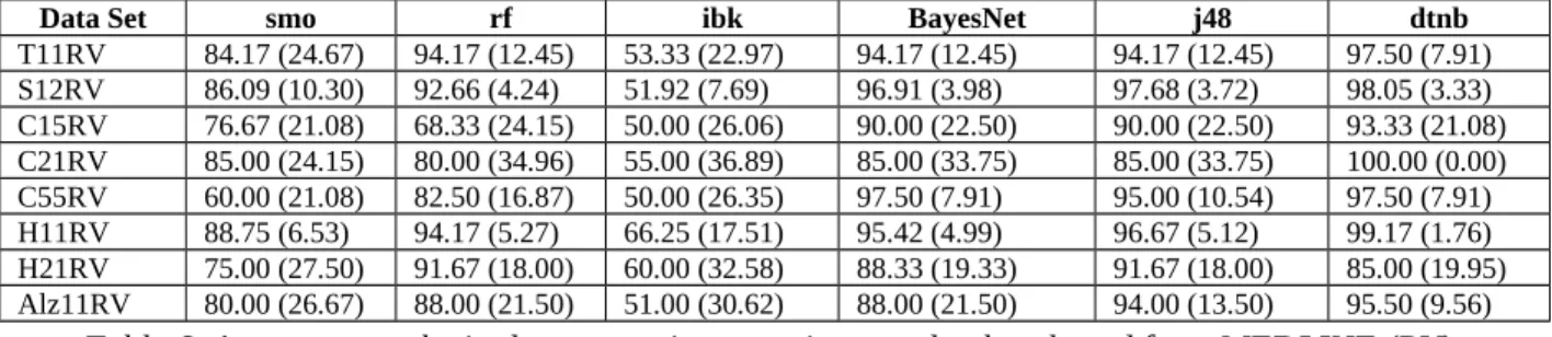
Data Set smo rf ibk BayesNet j48 dtnb T11RV 84.17 (24.67) 94.17 (12.45) 53.33 (22.97) 94.17 (12.45) 94.17 (12.45) 97.50 (7.91) S12RV 86.09 (10.30) 92.66 (4.24) 51.92 (7.69) 96.91 (3.98) 97.68 (3.72) 98.05 (3.33) C15RV 76.67 (21.08) 68.33 (24.15) 50.00 (26.06) 90.00 (22.50) 90.00 (22.50) 93.33 (21.08) C21RV 85.00 (24.15) 80.00 (34.96) 55.00 (36.89) 85.00 (33.75) 85.00 (33.75) 100.00 (0.00) C55RV 60.00 (21.08) 82.50 (16.87) 50.00 (26.35) 97.50 (7.91) 95.00 (10.54) 97.50 (7.91) H11RV 88.75 (6.53) 94.17 (5.27) 66.25 (17.51) 95.42 (4.99) 96.67 (5.12) 99.17 (1.76) H21RV 75.00 (27.50) 91.67 (18.00) 60.00 (32.58) 88.33 (19.33) 91.67 (18.00) 85.00 (19.95) Alz11RV 80.00 (26.67) 88.00 (21.50) 51.00 (30.62) 88.00 (21.50) 94.00 (13.50) 95.50 (9.56)
Table 6. Accuracy results in data sets using negatives randomly selected from MEDLINE (RV).
Ensemble Classifiers
An ensemble is a collection of models whose predictions are combined by weighted averaging or voting. According to (Dietterich, 2000) a necessary and sufficient condition for an ensemble of classifiers to be more accurate than any of its individual members is if the classifiers are accurate and diverse.
An ensemble of classifiers is a set of classifiers whose individual decisions are combined in some way (majority or voting) to classify new examples.
The main objective of ensemble classifiers is to achieve a better performance than the constituents classifiers. The literature (Opitz & Maclin, 1999), (Dzeroski & Zenko, 2004), (Homayouni & Hashemi & Hamzeh, 2010) refers that:
• Combining predictions of an ensemble is often more accurate than the individual classifiers that make them up
• The classifiers should be accurate and diverse
• An accurate classifier is one that has an error rate of better than random guessing (known as weak learners)
• Two classifiers are diverse if they make different errors on new data points
We have used the most common Ensembles available in the WEKA tool: Bagging, AdaBoost and Ensemble Selection for performing the experiments.
(Kotsiantis and Pintelas, 2004) states that bagging and boosting are among the most popular resampling ensemble methods that generate and combine a diversity of classifiers using the same learning algorithm for the base-classifiers.
Bagging
Bagging (Bootstrap aggregating) was proposed by (Breiman, 1996) and its basic idea is to generate several classifiers from a training set. These classifiers are generated independently. Bagging generates several samples from the original training data set using bootstrap sampling (Efron, 1996) and then trains a base classifier from each sample whose predictions are combined by a majority vote among the classifiers.
AdaBoost
In AdaBoost (Freund and Schapire, 1997) the performance of simple (weak) classifiers is boosted by combining them iteratively.
Boosting methods re-weight in an adaptively way the training based on the values of the previous base classifier.
Boosting is also a method based on combining several different classifiers. The main differences between Bagging and Boosting are: the way instance samples are generated, and the way final classification is performed.
In Bagging, the classifiers are generated independently from each other. The Boosting method uses a more refined way to sample the original training set, where the samples are chosen according to the accuracy of the previously generated classifiers. Each classifier generation takes into account the accuracy of the classifiers generated in the previous steps.
According to (Kotsiantis and Pintelas, 2004) boosting algorithms are considered stronger than bagging on noise free data. However, there are strong empirical indications that bagging is much more robust than boosting in noisy settings.
Ensemble Selection
Recently, ensemble selection (Caruana, 2004) was proposed as a technique for building ensembles from large collections of diverse classifiers. Ensemble selection uses more classifiers, allows optimizing to arbitrary performance metrics, and includes refinements to prevent overfitting to the ensemble training data a larger problem when selecting from more classifiers. Experimental Results with Ensemble Classifiers
For the Bagging and AdaBoost classifiers we need to specify a base learner. We have used the experimental work with the base classifiers described previously. For each base classifier and data set we use the parameter combination that achieved best results. Each base classifier used in the ensembles use the best combination of parameters. We have also developed a wrapper for the ensembles that automatically tunes ensemble-level parameters.
The Ensemble Selection algorithm allows us to specify the set of base learners as well as the best options for each individual learner.
The following tables show the results obtained with WEKA’a ensemble classifiers: Bagging, AdaBoost and Ensemble Selection over the same data sets used in Tables 2 and 3.
Data Set AdaBoost Bagging EnsembleSelection
T11NMV 51.67 (27.72) 65.00 (22.84) 46.67 (26.99) EC15NMV 98.00 (4.22) 95.27 (6.58) 97.09 (4.69) EC45NMV 81.29 (7.90) 68.36 (12.76) 65.36 (12.14) BP12NMV 97.15 (3.81) 96.33 (3.51) 93.52 (3.85) BP25NMV 95.69 (3.50) 93.06 (5.11) 90.47 (4.50) C35NMV 94.56 (7.78) 92.33 (9.11) 90.11 (11.04)
Data Set AdaBoost Bagging EnsembleSelection T11MRV 73.33 (23.83) 75.00 (15.21) 75.83 (19.02) S12MRV 98.85 (1.86) 98.43 (2.777) 98.05 (2.79) Alz11MRV 94.00 (9.66) 91.50 (11.07) 87.50 (21.76) C15MRV 76.67 (26.29) 73.33 (25.09) 48.33 (30.88) C21MRV 85.00 (33.75) 85.00 (24.15) 85.00 (33.75) C55MRV 82.50 (16.87) 82.50 (16.87) 80.00 (19.72) H11MRV 98.75 (2.01) 99.58 (1.32) 96.67 (4.30) H21MRV 81.67 (24.15) 73.33 (23.83) 81.67 (24.15)
Table 8 - Ensemble's Accuracy results in data sets using randomly selected examples sharing MeSH terms with the positive examples (MRV).
Data Set AdaBoost Bagging Ensemble
Selection T11RV 100.00 (0.00) 94.17 (12.45) 94.17 (12.45) S12RV 99.22 (1.65) 98.05 (3.33) 97.29 (3.65) C15RV 93.33 (21.08) 90.00 (22.50) 90.00 (22.50) C21RV 100.00 (0.00) 90.00 (21.08) 85.00 (33.75) C55RV 97.50 (7.91) 100.00 (0.00) 97.50 (7.91) H11RV 99.17 (1.76) 99.17 (1.76) 96.25 (4.99) H21RV 91.67 (18.00) 86.67 (21.94) 88.33 (19.33) Alz11RV 95.50 (9.56) 95.50 (9.56) 90.00 (19.44)
Table 9 - Ensemble's Accuracy results in data sets using randomly selected examples (RV).
A summary of the Accuracy results with all data sets and all algorithms, base algorithms and ensembles, can be found in Table 10. In Table 10 each cell is the average of the accuracies of each algorithm in all data set in the three “types” of data sets; using near misses (NMV); using randomly selected negatives sharing MeSH terms with the positive examples (MRV) and; using randomly selected negative examples (RV).
Algorithms NMV MRV RV smo 89,54 63,40 79,81 rf 89,11 73,25 86,54 ibk 89,16 56,17 56,54 BayesNet 77,04 78,89 92,37 J48 81,28 83,02 93,00 dtnb 78,78 82,96 96,23 AdaBoost 86,39 86,35 97,05 Bagging 85,06 84,83 94,20 Ensemble Selection 80,54 81,63 92,32
Table 10 - Algorithms accuracy average for NMVs, RMVs and RVs
As a global result we can see that all algorithms have in general very good performance well above the majority class predictor (except for ibk in MRV and RV data sets). The results also suggest that generating randomly the negative examples produces better results. As expected ensemble learners have a more higher and uniform performance than base learners.
Sensitivity Tests
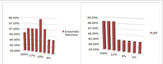
In some of the data sets the number of attributes is greater than the number of examples, which may cause the so called overfitting problem. As said previously the Ensemble Selection algorithm is known to perform well on avoiding overfitting. Apart from the use of such algorithm we investigate how performance (Accuracy) varies when reducing the number of attributes in the data sets. In fact we have pruned the attributes based on the number of positive documents they occur. For each original data set we have produced several version of it with increasing severity of pruning and apply the learning algorithms to those data sets.
Figure 4 shows the effect of attribute reduction on accuracy for Ensemble Selection algorithm (left side of the picture) and for J48 (right side of the picture). In general our experiments show that the variation on ensemble algorithms seems to be smaller than on base algorithms.
Figure 4 - Effect of attribute reduction. On the left side is Ensemble Selection algorithm and on the right side is J48.
CONCLUSIONS
This paper focuses on data set construction for posteriori classification of MEDLINE documents. Our study highlights the impact of three different ways to construct the data sets for posteriori classification. These three different ways are applied only to construct the negative examples. The first one is based on the concept of near miss values (NMV), which are examples that although negative are relatively close to the positive examples. The second approach is to use MeSH Random values (MRV) that is applied when we do not have enough negative near-miss examples (when negative examples are less than the number of positive examples) and add to this few or none examples some random negative examples from our LDB. However these examples are not just randomly selected, they must have some MeSH terms in common with the positive examples's MeSH terms that were previously processed. The last approach is to randomly select the negative examples from our LDB in equal number to the number of positive
examples. However in the second and third approach we guarantee that in these random negative examples there aren’t any positive examples.
We have generated several data sets with these different techniques. We have presented comparison tables, for these three techniques under study for six different categories: RNASES, Escherichia Coli, Blood Pressure, Alzheimer, Hemoglobin and Cholesterol. The categories were chosen by a biologist expert. These tables present the accuracy obtained performing a 10-fold cross validation and using different classification algorithms and the three different approaches (NMV, MRV and RV).
We have applied a collection of base learners and also ensemble learners. From the results presented in the accuracy tables, we can say that the use of randomly selected examples (RV) achieves, overall, better accuracy. We can also remark that ensembles learners performed better, as expected, than base learners.
REFERENCES
Ashburner M.. Gene ontology: Tool for the unification of biology. Nature Genetics, 25:25–29, 2000.
Breiman L.. Bagging Predictors. Machine Learning 24(2): 123-140, 1996.
Caruana R., Niculescu-Mizil A., Crew G., and Ksikes A.. Ensemble selection from libraries of models. In ICML, 2004.
Dietterich, T. G.. Ensemble methods in machine learning. First International Workshop on Multiple Classifier Systems, 2000.
Divoli A., Winter R., Pettifer S. and Attwood T.. 20. bioqspace: An interactive visualisation tool for clustering medline abstracts., 2005.
Dollah R., Seddiqui Md. H. and Aono M.. The effect of using hierarchical structure for classifying biomedical text abstracts. 2010.
Dzeroski S., and Zenko B.,. Is Combining Classifiers with Stacking Better than Selecting the Best One? Machine Learning, 54(3), 255–273, 2004.
Efron B., Tibshirani R.: An Introduction to the Bootstrap. New York: Chapman & Hall, 1993. Fellbaum C.. WordNet: An Electronical Lexical Database. The MIT Press, Cambridge, MA, 1998.
Freund Y. and Schapire R.E., A decision-theoretic generalization of on-line learning and an application to boosting. Journal of Computer and System Sciences, 55(1):119–139, August 1997. Frunza O., Inkpen D. And Tran T.. A machine learning approach for identifying disease-treatment relations in short texts. IEEE Trans. Knowl. Data Eng., 23(6):801–814, 2011. Gonçalves C.A., Gonçalves C.T., Camacho R. and Oliveira E. C.. The impact of preprocessing on the classification of medline documents. In Ana L. N. Fred, editor, Pattern Recognition in Information Systems, Proceedings of the 10th International Workshop on Pattern Recognition in Information Systems, PRIS 2010, In conjunction with ICEIS 2010, Funchal, Madeira, Portugal, June 2010, pages 53–61, 2010.
Gonçalves C. T., Camacho R. , Oliveira R., "From Sequences to Papers: An Information Retrieval Exercices", in Proc. of 2nd Workshop on Biological Data Mining and its Applications in Healthcare (BioDM 2011), colocated with 10th IEEE International Conference on Data Mining (ICDM 2011), Vancouver, Canada (to be presented), 2011.
Hall Mark, Frank Eibe, Holmes Geoffrey, Pfahringer Bernhard, Reutemann Peter, and Witten Ian H.. The weka data mining software: an update. SIGKDD Explor. Newsl., 11(1):10–18, 2009.
Homayouni H. Hashemi S. Hamzeh A., A Lazy Ensemble Learning Method to Classification, IJCSI International Journal of Computer Science Issues, Vol. 7, Issue 5, September 2010.
Hosford medical terms dictionary v3.0, 2004.
Indra N., Sarkar N., Schenk R., Miller H. and Norton C.. LigerCat: using ”MeSH Clouds” from journal, article, or gene citations to facilitate the identification of relevant biomedical literature. AMIA - Annual Symposium proceedings / AMIA Symposium. AMIA Symposium, 2009:563–567, 2009.
Imambi S. and Sudha T.. Classification of medline documents using global relevant weighing schema. International Journal of Computer Applications, 16(3):45–48, February 2011. Published by Foundation of Computer Science.
Kotsiantis S. and Pintelas P., Combining Bagging and Boosting, International Journal of Computational Intelligence, Vol. 1, No. 4 (324-333), 2004.
Opitz D. and Maclin R., Popular Ensemble Methods: An Empirical Study, Journal of Artificial Intelligence Research, vol.11, pp. 169-198, 1999.
Porter M. F.. An algorithm for suffix stripping. pages 313–316, 1997.
Rebholz-Schuhmann D., Pezik P., Lee V., Kim J-J, Del Gratta R., Sasaki Y., McNaught J., Montemagni S., MonachiniM., Calzolari N. and Ananiadou S. . Biolexicon: Towards a reference terminological resource in the biomedical domain. In Proceedings of the of the 16th Annual International Conference on Intelligent Systems for Molecular Biology (ISMB- 2008), 2008. Sehgal A. K., Sanmay D., Noto K., Milton H., Saier Jr. and Elkan C.. Identifying relevant data for a biological database: Handcrafted rules versus machine learning. IEEE/ACM Trans. Comput. Biology Bioinform., 8(3):851–857, 2011.
Settles B.. Abner: an open source tool for automatically tagging genes, proteins and other entity names in text. Bioinformatics, 21(14):3191–3192, 2005.
Wheeler D. L., Barrett T., Benson D. A, Bryant S. H., Canese K., Chetvernin V., Church D. M., Dicuccio M., Edgar R., Federhen S., Geer L. Y., Helmberg W., Kapustin Y., Kenton D. L., Khovayko O., Lipman D. J., Madden T. L., Maglott D. R., Ostell j., Pruitt K. D., Schuler G. D., Schriml L. M., Sequeira E., Sherry S. T., Sirotkin K., Souvorov A., Starchenko G., Suzek T. O., Tatusov R., Tatusova T. A., Wagner L., and Yaschenko E.. Database resources of the national center for biotechnology information. Nucleic Acids Res, 34(Database issue), January 2006. Zhou W., Smalheiser N. R. and Yu C.. A tutorial on information retrieval: basic terms and concepts. Journal of Biomedical Discovery and Collaboration, 1:2, March 2006.