Cointegration and Structural Breaks in the
PIIGS Economies
Nuno Ferreira#1, Rui Menezes#2, Sónia Bentes*3
#Department of Quantitative Methods, IBS-ISCTE Business School, ISCTE Avenida das Forças Armadas, Lisboa, Portugal
1
2
[email protected] *ISCAL
Avenida Miguel Bombarda, 20, Lisboa, Portugal
3
Abstract - Due to the economic recession which started in 2008, several members of the European Union became historically known as PIIGS. These states include Portugal, Italy, Ireland, Greece and Spain and if ombined together, they form the acronym PIIGS. The reason why these countries were grouped together is the substantial instability of their economies, which was an evident problem in 2009.
The reason why the five countries gained popularity is a serious concern within the EU, with regard to their national debts, especially for Greece. The latter country was involved in a controversial affair after allegedly falsifying its public financial data. In the year 2010, it was evident that the five states were in need of corrective action in order to regain their former financial stability.
Because of the dirty farm animal associated with the acronym, several country leaders from the financially troubled countries have voiced out disagreement with the use of the term. However, there are quite a number of reporters and columnists who still refer to it when talking about the widespread economic crisis within the European Union. Although some prominent politicians have criticized the practice, the use of the word is very hard to shake off.
Keywords ‐ Stock Markets Indices; Interest Rates; Structural Breaks; Cointegration; EU Sovereign Debt Crisis; PIIGS
1.
Introduction
As a result of the financial crisis, modeling the dynamics of financial markets is gaining more popularity than ever among researchers for both academic and technical reasons. Private and public economic agents take a close interest in the movements of stock market indexes, interest rates, and exchange rates in order to make investment and economic policy decisions. The most broadly
used unit root test used to identify stationarity of the time series studied in the applied econometric literature is the Augmented Dickey Fuller test (henceforth ADF).
However, several authors have stated that numerous price time series exhibit a structural change from their usual trend mostly due to significant policy changes. These economic events are caused by economic crises (e.g. changes in institutional arrangements, wars, financial crises, etc.) and have a marked impact on forecasting or analyzing the effect of policy changes in models with constant coefficients. As a result, there was strong evidence that the ADF test is biased towards null of random walk where there is a structural break in a time series. Such finding triggered the publication of numerous papers attempting to estimate structural breaks motivated by the fact that any random shock has a permanent effect on the system.
In the current context of crisis, this study analyzes structural break unit root tests in a 13 year time-window (1999-2012) for the five European markets under stress also known as PIIGS (Portugal (PT), Italy (IT), Ireland (IR), Greece (GR) and Spain(SP)), using the United States of America (US) as benchmark. The PIIGS countries gained popularity due to their national debts, especially for Greece. Despite several country leaders have voiced out disagreement with the use of the acronym associated with the dirty farm animal, the use of the word is very hard to shake off by a quite number of reporters and columnists.
Considering the problems generated by structural breaks, the unit root test Zivot and Andrews, 1992 (henceforth ZA) was employed to allow for shifts in the relationship between unconditional mean of the stock markets and interest
____________________________________________________________________________________ International Journal of Latest Trends in Finance & Economic Sciences IJLTFES, E‐ISSN: 2047‐0916
rate. The ZA unit root test captures only the most significant structural break in each variable. To confirm the presence of structural breaks detected by ZA test, this paper also employs the method developed by Bai and Perron (1998, 2001, 2003a and 2003b) (henceforth BP). This third test consistently estimates multiple structural changes in time series, their magnitude and the time of the breaks. However, it must be stressed that the consistency of the test depends on the assumption that time series are regime-wise stationary. This implies that breaks and break dates accurate with BP are only statistically reliable when the time series is stationary around a constant or a shifting level. If the time series is nonstationary, BP tests may detect that the time series has structural breaks.
A limitation of the ADF-type endogenous break unit root tests, e.g. ZA test, is that critical values are derived while assuming no break(s) under the null. Nunes et al. (1997) and Lee and Strazicich (2003) showed that this assumption leads to size distortions in the presence of a unit root with one or two breaks. As a result, one might conclude when using the ZA test that a time series is trend stationary, when, in fact, it is nonstationary with break(s), i.e. spurious rejections might occur.
To address this issue, Lee and Strazicich (2004) proposed a one-break Lagrange Multiplier (henceforth LM) unit root test as an alternative to the ZA test. In contrast to the ADF test, the LM unit root test has the advantage that it is unaffected by breaks under the null. These authors proposed an endogenous LM type unit root test which accounts for a change in both the intercept and also in the intercept and slope. The break date is determined by obtaining the minimum LM t-statistic across all possible regressions. More recently, several studies started to apply the LM unit root test with one and two structural breaks to analyze the time series properties of macroeconomic variables (e.g. Narayan, 2006; Chou, 2007; Lean and Smyth, 2007a, 2007b).
Based on the studies cited above, we concluded the first part of the analysis assuming that the break date is unknown and data-dependent. The distinct tests applied aimed to detect the most important structural breaks in the stock market and the interest rate relationship of all markets under analysis.
Having linked the source of the breaks found with some economic events during the time window under study, it was possible to advance with the second part of the analysis in which the main goal
was to explore a possible cointegration relationship between interest rates and stock market prices. Therefore, the Gregory and Hansen (1996) regime shift model (henceforth G-H) was used to find evidence of structural regime shifts that could explain the contamination of the severe EU debt crisis. The results identified the most significant structural breaks at the end of 2010 and consistently rejected the null hypothesis of no cointegration. Moreover, they showed that both the regional credit market and stock market have reached a nearly full integration in both pre and post crisis periods.
2.
Methodology
2.1 Zivot and Andrews test
The ZA is the most widely adopted endogenous one-break test. Building on Perron's (1989) exogenous break test, it only considers a break under the alternative but not under the null when carrying out unit root testing. Of the three types of ADF test proposed by Perron, the authors applied the one in which the Ha is a break in the intercept and in the slope coefficient on the trend at an unknown breakpoint. Estimating by OLS:
∆
Δ 1
Thus many sequential regressions are computed
where D1t (λ) and D2t (λ) change each time. The t-test
statistic (concerning γ=0) is also computed in each regression. Zivot and Andrews (1992) re-examined the Nelson-Plosser dataset and found a number of problems with the unit-root tests employed; thereafter, the literature documented an exhaustive list of empirical studies which employed this test (e.g. Ibrahim, 2009; Karunaratne, 2010; Ranganathan and Ananthakumar. 2010; Ramirez, 2013).
2.2 Bai and Perron test
In The Bai and Perron (1998, 2001, 2003a, 2003b) methodology to estimate and infer multiple mean breaks models was based on dynamic linear regression models. They estimate the unknown break points given T observations by the least squares principle, and provide general consistency and asymptotic distribution results under fairly weak conditions, allowing for serial correlation and heteroskedasticity. In Bai and Perron (1998) the authors developed a sequential procedure to test the null hypothesis of one structural change versus the alternative of one plus one break in a single
regression model. Thus, the pure structural change model is considered in several studies and is defined
as j = 1,…, m + 1, t0=0 and tm+1 = T. The dependent
variable is subject to m breaks and cj is the mean of
the series, rt for each regime j. The model allows for
general serial correlation and heterogeneity of the residuals across segments. The pure structural change model can be estimated as follows. For each
m-partition, the least squares estimate of cj is obtained
by minimizing the sum of squared residuals, where minimization occurs over all possible m-partitions.
Several authors have recently implemented the BP test for multiple break dates (e.g. McMillan and Ruiz, 2009; Yu and Zivot, 2011; Loscos et al., 2011; Zhou and Cao, 2011; Dey and Wang, 2012).
2.3 Lee and Strazicich test
The first part of this empirical analysis ends with the LS test also known as LM test due to Langrage multipliers. The main advantage over previous tests is that they are not affected by structural breaks under the null hypothesis because the critical values of the ADF-type endogenous break unit root tests (such as ZA and LP) were derived while assuming no break(s) under the null. The test employed in this paper (model A, known as the “crash model”) could be
briefly described considering: 1, , ,
where for 1, 1,2 and 0
otherwise. Consequently, it could be evidenced that DGP incorporated breaks under the null (β=1) and alternative hypothesis (β>1) as already noted. Making the value of β uncertain, we could rewrite the both hypotheses as
: ,
: . (2)
Where and are stationary error terms with for and 0 otherwise. The LM unit root test statistic is obtained from the following regression Arghyrou (2007) designed this component as the LM score principle. The LM test statistic is determined by testing the unit root null hypothesis that The LM unit root test determines the time location of the two endogenous breaks, whereas represent each combination of break points] using a grid search as follows: The break time should minimize this statistic.
Critical values for a single break and two-break cases are tabulated from Lee and Strazicich (2003, 2004) respectively. Another approach to searching for unit roots with breaks by allowing nonstationarity
in the alternative hypothesis is adopted in several studies following the Lee and Strazicich (2003, 2004) procedure testing.
2.4 Gregory and Hansen test
Gregory and Hansen (1996) used a residual-based test for cointegration in a multivariate time series with regime shifts; they proposed the ADF tests, which are intended to test the null hypothesis of no cointegration against the alternative of cointegration in the presence of a possible regime shift. This test examines whether there has been a one-time shift in the cointegration relationship by detecting any cointegration in the possible presence of such breaks and presents four different approaches. A single-equation regression with structural change starting with the standard model of cointegration (model 1):
, 1, … , (3)
In this case, if there is stated a long-run relationship, µ and α are necessarily defined as time-invariant. The G-H approach consider that this long-run relationship could shift to a new long long-run relationship by introducing an unknown shifting point that is reflected in changes in the intercept µ and/or changes to the slope α defining Model 2 and 3 in the following form (model 2 - level shift (C)):
, 1, … , (4)
This model represents a level shift in the cointegration relationship, and is modeled as a
change in the intercept µ variable. µ1.and µ2 represent
the intercept before and at the time of the shift. In order to account for the structural change, the authors introduced the dummy variable definition:
0 ,
1 . (5)
where the unknown parameter ∈ 0,1
represents the relative timing of the change point and [.] denotes integer part. Model 3: Level Shift with Trend (C/T):
, 1, … ,
In this model, the authors extended the
possibilities by introducing a time trend βt into the
level shift model. And finally, the model 4 - Regime Shift (C/S):
, 1, … , (7)
The last model integrates a shift in the slope vector, which permits the equilibrium relation to
rotate and a parallel shift. For this case, α1 is the
cointegrating slope coefficient before the regime
shift, and α2 is the change in the slope coefficients,
whereas is the cointegrating slope
coefficient after the regime shift.
Concerning the software, all routines applied were run with WinRATS Pro 8.0 and are available in Estima website.
2.5 Dataset
The variables under study cover daily data from April 1999 to December 2012 and are expressed in levels after a logarithmization procedure. For instance, the stock market price (Pi), the (Y1) and (Y10) are the government bond yield and the interest rates at 1 year and 10 years, respectively. All the three variables have been collected for each selected market (Portugal (PT), Spain (SP), France (FR), Ireland (IR), Italy (IT) and Greece (GR)) from the European countries under most stress in the recent years. We also included the US market as a benchmark. All data have been collected and are available online from Datastream database.
3.
Results and discussion
The results of the unit root testing procedures are presented in the tables below, starting with the price index (Pi variable) (Table 1) which was implemented using both the intercept and trend options (ZA test).
Table 1. Unit-root tests (variable Pi). (**) indicates critical values at 1%. The optimal lag length
was determined by SBC.
The corresponding time of the structural break (TB1 and TB2) for each variable is also shown in each test. For the Pi variable in the established crisis period, the ZA test fails to reject the null hypothesis of a unit-root at the 1 percent significance level in all countries except Greece. This means that the price index series of the remaining countries are
non-stationary. For the 1 year interest rate (variable Y1)
series (Table 2), the ZA test fails to reject the null hypothesis of a unit-root at 1 percent significance level US.
Table 2. Unit-root tests (variable Y1). (**) indicates critical values at 1%. The optimal lag length was
determined by SBC.
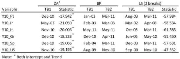
The analyses of the 10 year interest rate (variable Y10) series reveal that all countries are stationary meaning that this is not a good indicator to cointegrate (Table 3).
Table 3. Unit-root tests (variable Y10). (**) indicates critical values at 1%. The optimal lag length
was determined by SBC.
In light of these results, the cointegration hypothesis was tested with the Pi variable of all European countries (except GR) against the Y1 variable of US (Table 4). The structural break points defined through the different tests consistently coincide with important dates through the time-window analyzed, with special emphasis on the US.
According to Lee et al. (2006) and citing Ghoshray and Johnson (2010), by allowing for the possibility of a break in the null, the LM test can be considered genuine evidence of stationarity; this means that we can rely more on the break points calculated by the minimum LM test than those estimated by the remaining tests. This could lead to size distortion which increases with the magnitude of
Variable TB1 Statistic TB1 TB2 TB1 TB2 Statistic
Pi_Pt Aug‐03 ‐2.631 May‐01 Aug‐11 Feb‐06 Jul‐11 ‐1.384 Pi_Ir Aug‐04 ‐3.153 Jul‐05 Sep‐08 Oct‐08 May‐10 ‐1.664 Pi_It May‐08 ‐4.233 Nov‐04 Jul‐08 Mar‐07 Sep‐08 ‐1.519 Pi_Gr Nov‐05 ‐11.216**
Feb‐00 Nov‐05 Sep‐00 Nov‐05 ‐33.674 Pi_Sp Aug‐04 ‐3.012 Dec‐05 Oct‐08 Sep‐04 Aug‐11 ‐1.907 Pi_US May‐03 ‐3.217 May‐02 Jul‐05 Sep‐01 Jan‐03 ‐2.043 Note: a
Both Intercept and Trend
LS (2 breaks) ZAa
BP
Variable TB1 Statistic TB1 TB2 TB1 TB2 Statistic
Y1_Pt Sep‐07 ‐13.643**
Sep‐07 Jun‐12 Sep‐07 Aug‐11 ‐34.279 Y1_Ir Sep‐07 ‐16.770**
Sep‐07 Jun‐12 Dec‐04 Sep‐07 ‐45.173 Y1_It Dec‐10 ‐13.682**
May‐09 Jul‐12 Mar‐06 Aug‐11 ‐34.730 Y1_Gr Dec‐10 ‐9.454**
Jan‐01 Apr‐12 Aug‐01 Aug‐11 ‐29.893 Y1_Sp Sep‐07 ‐16.308**
Sep‐07 Jun‐12 Sep‐07 Aug‐11 ‐40.278 Y1_US Feb‐06 ‐2.048 Sep‐03 Apr‐08 Jul‐01 Nov‐02 ‐4.553 Note: a
Both Intercept and Trend
LS (2 breaks) ZAa
BP
Variable TB1 Statistic TB1 TB2 TB1 TB2 Statistic
Y10_Pt Dec‐10 ‐17.942**
Jan‐03 Mar‐11 Aug‐03 Mar‐11 ‐57.984 Y10_Ir May‐03 ‐21.050**
Feb‐03 Mar‐03 Mar‐02 Apr‐08 ‐58.534 Y10_It Nov‐10 ‐20.006** May‐11 May‐11 Oct‐03 Mar‐11 ‐61.385 Y10_Gr Dec‐10 ‐18.223**
Dec‐10 Apr‐11 Jun‐05 May‐10 ‐55.450 Y10_Sp Dec‐10 ‐19.066**
Feb‐04 Mar‐11 Dec‐03 Mar‐11 ‐57.631 Y10_US Nov‐10 ‐19.195**
Aug‐09 Nov‐10 Sep‐00 Nov‐10 ‐47.352 Note: a
Both Intercept and Trend
LS (2 breaks) ZAa
the break; this does not occur with the LM test as a different detrending method is used.
Following these assumptions and focusing on the structural break points identified by the LM test (two breaks), all dates related to 2001-2003 reveal the economic impact of the September 11 attacks on the US, namely in New York City and Washington D.C. in 2001 and the repercussions in the following years with the concerted military action against Iraq.
Further, a mild recession in 2001, caused partly by the bursting of the dot-com bubble, prompted the Fed (led by Chairman Alan Greenspan) to lower the target federal funds rate from 6% to 1.75% in an effort to stimulate employment. The Fed kept interest rates low for the next two years; it dropped to just 1% - the lowest rate in 50 years - in summer 2003, and only rose again one year later. By late 2003, the US was in the midst of the most serious world economic setback, originated by the credit boom (interest rates were at a 50-year-low and mortgage credit stood at an all-time high) and the housing bubble (prices had exceeded all previous levels).
The first half of 2004 was characterized by a trend towards gradual economic recovery. However, there were still some obstacles hindering the growth of the world economy; for example, a rise in the price of oil per barrel to record high contributed to raise expectations in the major economic areas.
The marked depreciation of the euro against the dollar from May 2005 could have also played a role. In the run-up to this decision, the ECB had considerably stepped up its use of moral suasion to signal its readiness to raise interest rates “at any time”.
Meanwhile, when the downturn in housing prices finally began in 2006, everyone had difficult in repaying their mortgages as home equity loans shrank. Subprime borrowers were, by definition, more prone to default on their mortgages than the average person. The resulting wave of subprime foreclosures fueled the aforementioned downward spiral of prices, as it prompted a glut in housing supply and a contraction of housing demand.
By 2007, more than just a few farsighted economists were noting that the unprecedented rise in housing prices might be an unsustainable bubble (though most still underestimated the bubble’s economic significance).
In 2008, developments took a turn for the worse, and the growth slowdown became acuter. In early 2009, the conclusion was that this would be a deeper recession than the average of “Big Five” (those in Spain, 1977; Norway, 1987; Finland, 1991; Sweden, 1991 and Japan, 1992). The conjuncture of elements is illustrative of the two channels of contagion: cross-linkages and common shocks.
There can be no doubt that the US financial crisis of 2007 spilled over into other markets through direct linkages. The governments of emerging markets had experienced stress, although of mid-2009 sovereign credit spreads had narrowed substantially in the wake of massive support from rich countries for the IMF fund. European banks began to face liquidity problems after August 2007, and German banks continued to lend heavily to peripheral borrowers in the mistaken belief that peripheral countries were a safe outlet. Net exposure rose substantially in 2008. Speculators focused on Greek public debt on account of the country’s large and entrenched current account deficit as well as because of the small size of the market in Greek public bonds. Greece was potentially the start of speculative attacks on other peripheral countries – and even on countries beyond the Eurozone, such as the UK – that faced expanding public debt.
Greece thus found itself in a very difficult position in early 2010 and imposed cuts and raised taxes in order to pay high interest rates to buyers of its public debt. The country was able to access markets in January and March 2010, but the rate of interest was high on both occasions - well in excess of 6 percent. On 2 May 2010, the EU announced a support package for Greece, put together in conjunction with the IMF fund. Lapavitsas et al. (2012) documented that the sovereign debt crisis that broke out in Greece at the end of 2009 was fundamentally due to the precarious integration of peripheral countries in the Eurozone. Its immediate causes, however, lie with the crisis of 2007-9.
The result in the Eurozone was a sovereign debt crisis, exacerbated by the structural weaknesses of monetary union. Meanwhile, with the global economy likely to perform indifferently in 2010-11 and given the high regional integration of European economies, exports were unlikely to prove the engine of growth for Europe as a whole. The austerity policy ran the risk of resulting in a major recession.
These are but a few insights into the dates of structural breaks given in Tables 1 to 3. The crisis in the different financial markets (e.g. credit, debt, derivatives, property and equity) are just the tip of the iceberg of a severe financial crisis of huge proportions worldwide. In Europe, the sovereign debt crisis should be considered as spreading across a broad front the instability of each country, leading to an employment crisis and in turn a social crisis, and eventually turning into a political crisis.
The Greek case is not discussed further in this study due to the deep crisis in which the country is submerged. This trend can be observed in both the Pi and the Y1 variables (Tables 1 and 2).
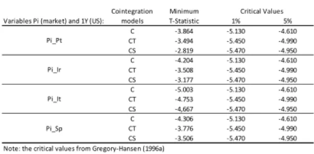
Table 4. Cointegration results
The cointegration hypothesis was tested by performing the relationship between the stock market prices and interest rates (Table 4). Bivariate cointegration was considered for this purpose, allowing for structural break tests between the price indexes of each stock market and the interest rate at 1 year of US market benchmark.
This test detects regime-shift as well as stable cointegration relationships. Thus, the rejection of the null hypothesis does not entangle the instability of the cointegration relationship. The differentiation of these situations is made using stationarity tests and with the structural breaks previously presented. It is possible to infer the US influence on the European equity markets through the timing of structural breaks (Tables 1 to 3) and because both variables show prolonged upward and downward movements (resumed in Table 4).
The corresponding time of the structural break (TB1 and TB2) for each variable is also shown in each test. For the Pi variable in the established crisis period, the ZA test fails to reject the null hypothesis of a unit-root at the 1 percent significance level in all countries except Greece. This means that the price
index series of the remaining countries are non-stationary.
4.
Conclusion
This paper explored possible structural changes in the stock market and interest rate variables (in PIIGS states) as well as the relationship between them. With this purpose, first the ZA and the LS (2 breaks) were employed to test for the presence of structural breaks with unknown timing in the individual series; multiple structural breaks was then detected with BP test. Secondly, the G-H test was used for cointegration between stock market prices and the interest rates for the European markets under stress and infected by the vast sovereign debt crisis since 2003. The results effectively revealed that there was a relationship between the two variables in all analyzed countries which implies important economic repercussions. Conducting monetary policy by targeting a monetary aggregate requires reliable quantitative estimates of the demand for money determined by the interest rate behavior.
An examination of the crisis reveals that economies are already quite integrated, and this resulted in its spread from the US to the rest of the world.
References
[1] Arghyrou, M.G., 2007. The price effects of joining the Euro: Modeling the Greek experience using non-linear price-adjustment models. Applied Economics, 39(4), 493-503. [2] Bai, J., Perron, P., 2003b. Critical values for multiple structural change tests. Econometrics
Journal, 6, 72-78.
[3] Bai, J., Perron, P., 2003a. Computation and analysis of multiple structural change models.
Journal of Applied Econometrics, 18, 1-22.
[4] Bai, J., Perron, P., 2001. Multiple structural
change models: A simulation analysis.
Manuscript, Boston University.
[5] Bai, J., Perron, P., 1998. Estimating and testing linear models with multiple structural changes.
Econometrica, 66, 47-78.
[6] Chou, W.L., 2007. Performance of LM-type unit root tests with trend break: A bootstrap approach. Economics Letters, 94(1), 76-82. Cointegration Minimum
Variables Pi (market) and 1Y (US): models T‐Statistic 1% 5%
C ‐3.864 ‐5.130 ‐4.610 CT ‐3.494 ‐5.450 ‐4.990 CS ‐2.819 ‐5.470 ‐4.950 C ‐4.204 ‐5.130 ‐4.610 CT ‐3.508 ‐5.450 ‐4.990 CS ‐3.177 ‐5.470 ‐4.950 C ‐5.003 ‐5.130 ‐4.610 CT ‐4.753 ‐5.450 ‐4.990 CS ‐4,667 ‐5.470 ‐4.950 C ‐4.306 ‐5.130 ‐4.610 CT ‐3.776 ‐5.450 ‐4.990 CS ‐3.506 ‐5.470 ‐4.950 Note: the critical values from Gregory‐Hansen (1996a) Pi_Pt Pi_Ir Pi_It Pi_Sp Critical Values
[7] Dey, M.K., Wang, C., 2012. Return spread and liquidity: Evidence from Hong Kong ADRs.
Research in International Business and Finance, 26(2), 164-180.
[8] Ghoshray, A., Johnson, B., 2010. Trends in world energy prices. Energy Economics, 32, 1147-1156.
[9] Gregory, A.W., Hansen, B.E., 1996. Tests for cointegration in models with regime and trend shifts. Oxford Bulletin of Economics and
Statistics, 58, 555-560.
[10] Ibrahim, S., 2009. East Asian Financial Integration: A Cointegration Test Allowing for Structural Break and the Role of Regional Institutions. International Journal of Economics
and Management, 3(1), 184-203.
[11] Karunaratne, N.D., 2010. The sustainability of Australia’s current account deficit – A reappraisal after the global financial crisis.
Journal of Policy Modeling, 32, 81-97.
[12] Lapavitsas, C., 2012. Crisis in the Eurozone. Verso Books.
[13] Lean, H.H., Smyth, R., 2007b. Are Asian real exchange rates mean reverting? Evidence from univariate and panel LM unit root tests with one and two structural breaks. Applied Economics, 39, 2109-20.
[14] Lean, H.H., Smyth, R., 2007a. Do Asian stock markets follow a random walk? Evidence from LM unit root tests with one and two structural breaks. Review of Pacific Basin Financial
Markets and Policies, 10(1), 15-31.
[15] Lee, J., List, J.A., Strazicich, M.C., 2006. Non-renewable resource prices: deterministic or stochastic trends? Journal of Environmental
Economics and Management, 51(3), 354-370.
[16] Lee, J. and Strazicich, M.C., 2004. Minimum
LM unit root test with one structural break.
Appalachain State University, Department of Economics, Working Paper No 17.
[17] Lee, J., Strazicich, M.C., 2003. Minimum Lagrange multiplier unit root test with two structural breaks. The Review of Economics
and Statistics, 85(4), 1082-1089.
[18] Loscos A.G., Montañés, A., Gadea, M.D., 2011. The impact of oil shocks on the Spanish economy. Energy Economics, 33(6), 1070-1081. [19] McMillan, D., Ruiz, I., 2009. Volatility
persistence, long memory and time varying unconditional mean: Evidence from 10 equity indices. The Quarterly Review of Economics
and Finance, 49, 578-595.
[20] Narayan, P.K., 2006. The behavior of US stock prices: evidence from a threshold autoregressive model. Mathematics and Computers in Simulation 71, 103-108.
[21] Nunes, L.C., Newbold, P., Kuan, C.M., 1997. Testing for unit roots with breaks: Evidence on the Great Crash and the unit root hypothesis reconsidered. Oxford Bulletin of Economics and Statistics 59(4), 435-448.
[22] Perron, P., 1989. The Great Crash, the Oil Price Shock, and the Unit Root Hypothesis. Econometrica 57(6), 1361-1401.
[23] Ramirez, M., 2013. Remittances and Economic Growth in Mexico: An Empirical Study with Structural Breaks. Working Paper 13-06. Trinity College Department of Economics.
[24] Ranganathan, T., Ananthakumar, U., 2010. Give it a break. 30th International Symposium on Forecasting, San Diego, USA.
[25] Yu, W.C., Zivot, E., 2011. Forecasting the term structures of Treasury and corporate yields using dynamic Nelson-Siegel models.
International Journal of Forecasting 27(2), 579-591.
[26] Zhou, D., Cao, J., 2011. A quantitative assessment on the evolution of Chinese energy and US. Renewable and Sustainable Energy Reviews 15(1), 886-890.
[27] Zivot, E., Andrews, D.W.K., 1992. Further Evidence on the Great Crash, Oil Price Shock and the Unit Root Hypothesis. Journal of Business and Economic Statistics 10, 251-270.