Assessment of the spatio-temporal variability and estimation accuracy of drought indices and evapotranspiration

(1)

2019

UNIVERSIDADE DE LISBOA FACULDADE DE CIÊNCIAS

Assessment of the spatio-temporal variability and estimation accuracy of drought indices and evapotranspiration

“Documento Definitivo”

Doutoramento em Ciências Geofísicas e da Geoinformação Especialidade de Meteorologia

Diogo Miguel dos Santos Martins

Tese orientada por:

Professor Doutor Carlos Alberto Leitão Pires Professor Doutor Luis Santos Pereira Professora Doutora Ana Ambrósio Paulo

(2)

(3)

2019

UNIVERSIDADE DE LISBOA FACULDADE DE CIÊNCIAS

Assessment of the spatio-temporal variability and estimation accuracy of drought indices and evapotranspiration

Doutoramento em Ciências Geofísicas e da Geoinformação

Especialidade de Meteorologia

Diogo Miguel dos Santos Martins

Tese orientada por:

Professor Doutor Carlos Alberto Leitão Pires, Professor Doutor Luis Santos Pereira, Professora Doutora Ana Ambrósio Paulo

Júri: Presidente:

● Doutor João Manuel de Almeida Serra, Professor Catedrático Faculdade de Ciências da Universidade de Lisboa.

Vogais:

● Doutora Elsa Estevão Fachadas Nunes Moreira, Professora Auxiliar Faculdade de Ciências e Tecnologia da Universidade Nova de Lisboa; ● Doutor João Carlos Andrade dos Santos, Professor Auxiliar com Agregação

Escola de Ciências e Tecnologia da Universidade de Trás-os-Montes e Alto Douro; ● Doutora Paula Cristina Santana Paredes, Professora Auxiliar

Instituto Superior de Agronomia da Universidade de Lisboa; ● Doutor Carlos Alberto Leitão Pires, Professor Auxiliar

Faculdade de Ciências da Universidade de Lisboa (orientador).

Documento especialmente elaborado para a obtenção do grau de doutor

(4)

(5)

ii

Acknowledgments

First, I would like to thank my advisors, Professor Carlos Pires, Professor Luis Santos Pereira and Professor Ana Paulo. Your support, guidance, shared knowelge and friendship was invaluable during this PhD.

A sincere thank you to Dr. Paula Paredes, for the all friendship and help in this journey and to Professor Teresa do Paço for the patience and freedom given in this past year, which allowed me to finish this Thesis.

I also want to thank all the Professors and collegues I had the pleasure to work within the framework of this Thesis: Doctor Tayeb Raziei, Doctor Elsa Moreira, Mr. Xiaodong Ren, Doctor Abdelaaziz Merabti and Professor Jorge Cadima.

I acknowledge the support provided by the Fundação para a Ciência e Tecnologia under the grant SFRH/BD/92880/2013.

(6)

iii

Agradecimentos

Agradeço, também, aos meus excelsos, caros e nunca assaz louvados amigos. A Cavia, a uma amizade que, espero, não tenha fim. À Daniela, Maria e Virgilio, por tornarem as semanas de trabalho mais divertidas e interessantes.

Por último um agradecimento especial aos meus pais, por tudo. Pelo apoio e pelo carinho, sem duvida que sem eles não conseguiria concluir este trabalho. À minha família e, claro, à Zoey.

(7)

(8)

v

Abstract

Understanding the spatial and temporal variability of droughts is important to improve drought predictability and ultimately to support drought risk management in agriculture. Several studies were developed, to better understand drought characteristics and variability. For that, the Standardized Drought Index (SPI) was used to identify the main spatial and temporal patterns of drought variability in Portugal, to search for regions with similar drought variability in continental Portugal and significant cycles using a Fourier analysis applied to the SPI, which revelead cycles of 6 and 9.4 years, likely influenced by the North Atlantic Oscillation (NAO) and two stable sub-regions, in the northern and southern regions of Portugal. Moroever, another study using the SPI suggested that for drought monitoring, when using non-stationary time series of precipitation, the reference period used for obtaining the Gamma distribution parameters is important.

Altough the SPI is widely used it only uses precipitation, however, for assessment of agricultural drought conditions indices such as the Palmer Drought Severity Index and its modification for the Mediterranean region, the MedPDSI, may be a better option since they consider the interaction between precipitation and evapotranspiration within a soil water balance. For that reason, in this Thesis the different methodologies to estimate evapotranspiration, on a monthly and daily basis, were tested for different climates conditions.

The results obtained during the course of this Thesis led to the development of the MedPDSI. The MedPDSI improves upon the PDSI mainly by modifying its soil water balance, adapting it to the Mediterranean climate conditions. MedPDSI was computed using reference evapotranspiration based on reanalysis data. Comparing to the PDSI, with the MedPDSI, droughts are generally identified earlier, are longer and more severe, which is an advantage for drought management, since coping management schemes can be implemented earlier to manage drought impacts and thus mitigating its potential negative consequences.

Keywords: drought indices; MedPDSI; Reanalysis products; reference evapotranspiration; soil water balance

(9)

(10)

vii

Resumo

A água é um bem essencial para a existência de vida, determinante para o desenvolvimento socioeconómico e para a manutenção dos ecossistemas. O rápido crescimento económico e populacional tem provocado uma enorme pressão sobre os recursos hídricos. Muitos países vivem, atualmente, em condições extremas de escassez de água, com graves consequências humanitárias, económicas e ambientais. Embora as ações do homem tenham um peso significativo na disponibilidade e qualidade da água existem fatores naturais, difíceis de controlar, como a ocorrência de secas que agravam consideravelmente o fenómeno da escassez. Estes impactos, são ainda mais severos em regiões áridas e semiáridas com uma elevada variabilidade climática.

As secas são um fenómeno climático extremo que provocam desequilíbrios naturais e temporários na disponibilidade de água, de ocorrência aleatória, severidade incerta sendo encaradas como risco e como desastre. As características das secas (duração, severidade e extensão espacial) determinam a sua importância a nível da região, e é fundamental um melhor conhecimento do fenómeno para que seja possível promover uma melhor gestão dos recursos de forma preventiva, tentando atenuar os impactos negativos das secas. Nas últimas décadas vários índices de seca têm sido desenvolvidos para a caracterização e compreensão das secas em todo o Mundo. Os mais amplamente estudados para esse efeito têm sido o Standardized Precipitation Index (SPI) e o Palmer Drought Severity Index (PDSI) e ambos são utilizados nesta Tese, bem como uma modificação do PDSI para as condições mediterrânicas, o MedPDSI, que é proposta visando a criação de um índice de seca, adaptado e calibrado às condições climáticas de Portugal e do Mediterrâneo, usando o olival tradicional como cultura de referência.

Compreender a variabilidade espacial e temporal das secas é importante para melhorar a sua previsibilidade e tem como objetivo o apoio à gestão de risco às secas. No âmbito desta Tese, foram desenvolvidos estudos com o objetivo de melhor compreender a variabilidade da seca. No Capítulo 2 estudou-se a estabilidade dos padrões espaciais e temporais de secas em Portugal aplicando a Análise de Componentes Principais ao SPI para várias escalas temporais, calculado para três conjuntos de dados relativos ao período comum de 1950-2003: (1) conjunto de séries de precipitação mensal provenientes de 193 estação meteorológicas e udométricas e (2) Dados de precipitação mensal em grelha,

(11)

viii

provenientes das bases de dados GPCC e PT02, com resoluções horizontais de 0.5º e 0.2º, respetivamente. Os resultados sugerem elevada estabilidade dos padrões espaciais de seca, independentes da escala temporal do SPI, da base de dados usada e do período de referência considerado para o cálculo, identificando-se duas sub-regiões no Norte e Sul de Portugal como os principais modos de variabilidade das secas. É identificada no Centro-Este de Portugal uma terceira sub-região, mas apenas quando usando o SPI-24 calculado com a base de dados PT02. No âmbito da análise da variabilidade temporal do SPI em Portugal, analisou-se ainda a ciclicidade das secas recorrendo a uma análise de Fourier aplicada a 74 séries temporais do SPI-12 com 66 anos. Os ciclos significativos mais frequentes foram identificados e analisados para o mês de Dezembro. Os resultados mostraram que as periodicidades variam espacialmente em Portugal, apontando, contudo, para um ciclo de 6 anos comum a todo o país e um ciclo de 9.4 anos muito mais frequente no centro e sul de Portugal. Ambos os ciclos estão provavelmente relacionados com a influência da Oscilação do Atlântico Norte sobre a ocorrência e gravidade das secas em Portugal.

No Capítulo 3 estudou-se também o efeito da variabilidade da precipitação sobre o SPI efetuando a partição de 10 séries longas de precipitação, em sub-períodos e obtendo as séries de SPI para cada sub-período. Calcularam-se, assim, limiares de precipitação correspondentes às categorias de seca moderada, severa e extrema do SPI. As mudanças dos padrões de precipitação refletem-se no valor destes limiares. Em 8 das 10 localidades estudadas os limiares de precipitação do período mais recente, 1976-2007, são inferiores aos limiares equivalentes do período antecedente. Os limiares de precipitação permitem avaliar a magnitude do défice, expresso em altura de precipitação, complementando informação fornecida pelo índice de seca SPI.

O SPI é um índice de seca padronizado que é calculado recorrendo apenas a dados de precipitação. Existem outros índices que consideram não só a influência da precipitação como da evapotranspiração, como por exemplo o Palmer Drought Severity Index (PDSI) que combina precipitação e evapotranspiração num balanço hídrico e, portanto, poderá ser mais adequado para a caracterização da seca na agricultura. Portanto, no Capítulo 3 estudou-se também o impacto da variação temporal a longo prazo das secas, usando o PDSI. Para tal usou-se dados da reanálise do Século XX NOAA-CIRES, previamente validados com dados observados, que abrange o período 1851-2014, com uma resolução espacial de 2.0ºx2.0º. Dados de temperatura máxima e mínima, humidade relativa,

(12)

ix

velocidade do vento e radiação foram retirados da reanálise do Século XX para calcular a evapotranspiração de referência pelo método da FAO-56, que, juntamente, com dados de precipitação provenientes de estações meteorológicas foram usados para o cálculo do PDSI. Para avaliar como a variabilidade de longo prazo do clima influencia a identificação de eventos secos pelos índices de seca, cinco períodos de calibração diferentes foram selecionados para estimar os valores potenciais de evapotranspiração, escoamento superficial, recarga de água no solo e perdas do balanço hídrico do PDSI. A mesma análise foi feita em paralelo com o SPI com uma escala temporal a 9 meses, usando os mesmos 5 períodos de calibração para a estimação dos parâmetros da função de distribuição do SPI. Os resultados mostraram índices distintos, dependendo dos períodos de calibração usados. Com os mesmos padrões para todas as localizações estudas, quando os índices de seca foram calibrados com o período mais recente (1974-2014), a quantidade de eventos de seca (severa ou extrema) identificados foi menor, tanto no PDSI e SPI-9, quando comparado com os índices calculados com os outros períodos de calibração. Contudo a deteção de eventos húmidos extremos e severos identificados foi maior quando os índices de seca foram calculados usando este período. Em contraste, se o período de calibração selecionado foi o período 1892-1932, o oposto ocorreu com uma maior quantidade de eventos secos detetados e menor frequência dos húmidos. Estes resultados mostraram a importância que a seleção do período de calibração tem tanto para o PDSI quanto para o SPI-9.

O impacto nos índices de seca como o PDSI da seleção do método usado para o cálculo da evapotranspiração é relevante e não deve ser negligenciado. Tradicionalmente o PDSI usa a evapotranspiração potencial obtida com recurso à equação de Thornthwaite. Contudo, existem outros métodos, de base física, como é caso da equação da evapotranspiração de referência calculada pelo método da FAO-56, que permitem estimações mais corretas da evapotranspiração embora necessitem de dados relativos à temperatura máxima e mínima, radiação solar, velocidade do vento e humidade relativa, que muitas vezes não estão disponíveis. No Capítulo 4 compararam-se três metodologias de cálculo de evapotranspiração, nomeadamente, o método da FAO-56 usando as cinco variáveis enumeradas anteriormente e duas equações baseadas somente em temperatura, usando dados diários e mensais para o período 1981-2012 na região da Mongólia interior permitindo a análise dos diferentes métodos em vários tipos de clima. Os resultados do Capítulo 4 mostraram que os métodos baseados em temperatura para o cálculo da

(13)

x

evapotranspiração são insuficientes para descrever corretamente a sua variabilidade e amplitude em todos os tipos de clima. Seguindo esses resultados, no Capítulo 5, produtos de reanálise foram testados como uma alternativa quando dados in situ não estão disponíveis, levando à conclusão de que dados climáticos da reanálise com correção de de viés são uma boa alternativa às observações para estimativas da evapotranspiração de referência mensal e diária.

Seguindo os resultados dos Capítulos anteriores, o PDSI foi modificado para responder melhor às condições do clima em Portugal (Capítulo 6). Esta modificação, o MedPDSI, melhora o PDSI principalmente modificando o seu balanço hídrico, adaptando-o às condições climáticas do Mediterrâneo. A evapotranspiração de referência foi calculada recorrendo a um conjunto de dados de reanálise e de dados observados, de modo a corrigir o viés nas variáveis de superfície, cuja performance foi aferida no Capítulo 5 e seguindo a metodologia de correção de viés testada, também, no Capítulo 5. Os resultados mostraram que o balanço hídrico do MedPDSI apresentou diferenças relevantes quando comparado ao do PDSI. A evapotranspiração real (ETact) do MedPDSI, apresentou uma

variabilidade mais realista, principalmente na transição dos meses secos para os húmidos quando comparado com a ETact do PDSI. Mais ainda, as secas identificadas com o

MedPDSI começam, geralmente, mais cedo, são mais longas e mais severas, o que é uma vantagem para a gestão da seca, já que os sistemas de gestão do risco de seca poderão ser implementados mais cedo para melhor gerir os seus impactos, mitigando as potenciais consequências negativas de eventos secos.

Palavras-chave: índices de seca; MedPDSI; produtos de reanálise; evapotranspiração de referência; balanço hídrico do solo.

(14)

xi

List of Acronyms, abbreviations and symbols

1 shape parameter ()

PRÊ expected precipitation to maintain normal climate conditions (mm) α̂ _l shape parameter estimator ()

β̂ _l scale parameter estimator ()

𝐸𝑇̂𝑜 estimated values of reference evapotranspiration (mm)

𝜌̂ 𝑗 estimated multiple regression coefficients ()

𝜙̃ estimators of 𝜙 () s_O2 variance of O ()

Xi severity of the event relative to the current month ()

X_i-1 severity of the event relative to the previous month ()

γl asymmetry ()

𝐼𝑗 periodogram function of the j-th periodic component ()

𝐾̃ first approximation of the climatic characteristic ()

𝑂̅ (in the same units as the variables used in the linear regression) 𝑃̅ mean value of the dependent variable vector (in the same units as the

variables used in the linear regression)

𝑃̂ predicted values of P (in the same units as the variables used in the linear regression)

𝑅2 coefficient of determination computed with the ordinary least squares ()

𝑔𝐴𝐵 congruence coefficient ()

𝑔𝑗 statistical test that tests for he significance of the j-th periodic

component ()

𝑦_𝑡 general model for a cyclic fluctuation () 𝜀_𝑡 white noise process ()

𝜃𝑗 amplitude of the j-th periodic component (Hz)

µ expected value (in the same units as the variables)

a intercept of a linear regression (in the same units as the variables used in the linear regression)

AI aridity index () AMJ April - May- June

ANN artificial neural networks AO arctic oscillation

ARIMA auto regressive integrated moving averages ASW available soil water (mm)

aT dew point temperature correction based on aridity (℃)

b slope of a linear regression ()

b0 coefficient of regression of the regression forced to the origin ()

bjA loading from the rotated loading vector A from one solution ()

bjB loading from the rotated loading vector B from one solution ()

c extreme dry (c= -4) and wet events (c=4) ()

c(t) difference between the mean values of the P and O (mm) cdf cumulative distribution function

CDI combined drought indicator

COTR centro operativo e tecnológico de regadio CovOP covariance between the values O and P ()

CP calibration period CRU Climate Research Unit

D moisture departure mm month-1) DFJ December–January–February

(19)

xvi DP deep percolation (mm) DTS deterministic trend scheme ea actual vapor pressure (kPa)

ECMWF European center for medium range weather forecasts EDO European drought observatory

EF modeling efficiency () ENSO El Niño–southern oscillation es saturation vapor pressure (kPa)

ET Evapotranspiration (mm) ETact actual evapotranspiration (mm)

ETc crop evapotranspiration (mm)

ETo grass reference evapotranspiration(mm)

ETr ASCE alfalfa reference evapotranspiration (mm)

FAO food and agriculture organization

FAO-PM food and agriculture Organization Pennam-Monteith reference evapotranspiration equation

fin at the end of the month ()

FTO regression forced to the origin (mm) GCM global circulation models

GG Granger and Gray

GPCC Global Precipitation Climatology Centre GWP Global Water Partnership

HS Hargreaves-Samani evapotranspiration equation ini in the beginning of the month ()

IPMA instituto português do mar e da atmosfera JAS July – August - September

JFM Jannuary- February – March

JJA June-July-August

K climatic characteristic ()

K´ climatic coefficient ponderation factor () Kc crop coefficient ()

Kcb basal crop coefficient ()

Kcor adjustment coefficient of Ke according to soil characteristics ()

Ke soil evaporation coefficient ()

KPSS test Kwiatkowski–Phillips–Schmidt–Shin test kRs empirical radiation adjustment coefficient

L soil water loss (mm)

LAS SAF Land Surface Analysis - Satellite Applications Facility Ls water loss in the surface layer (mm)

Lu water loss in the underlying layer (mm)

m n/2 if n is even or m = (n – 1)/2

MAM March-April-May

MedPDSI modification of the PDSI for the Mediterranean climate ()

MK Mann-Kendall test

MM5 Fifth-Generation Penn State/NCAR Mesoscale Model MMK modified Mann-Kendall test

MPDSI modified PDSI ()

MSE mean square error (in the same units as the variables used in the linear regression)

(20)

xvii NAO north Atlantic oscillation

NCEP/NCAR national center for environmental prediction/national center for atmospheric research

NCEP2 NCEP–DOE AMIP-II Reanalysis

NDVI normalized difference vegetation index () NRMSE Normalized root mean square error ()

Ns maximum possible duration of sunshine or daylight hours (h)

ns actual duration of sunshine (h)

O vector with the independent variables (in the same units as the variables used in the linear regression)

OBS observations

OLS ordinary least squares ()

OND October – November - December OYT optimal yield threshold (mm) p duration factor associated to Xi-1 ()

P vector with the dependent variables (in the same units as the variables used in the linear regression)

p’ soil water depletion fraction for no stress p0 false alarm probability ()

PBIAS percent bias (%)

PC principal componente

PCA principal component analysis pdf probability distribution function PDSI Palmer drought severity index () PDSI2nd second percentile of the PDSI series

PDSI98th 98th percentile of the PDSI series

PET potential evapotranspiration (mm) PHDI Palmer hydrological drought index ()

pj wavelength of the j-th periodic component ()

PL potential loss (mm)

PLs potential loss in the surface layer (mm)

PLu potential loss in the underlying layer (mm)

PM-ETo reference evapotranspiration computed using the FAO-PM equation

(mm)

PMT FAO-PM equation using temperature data only PP Phillips and Perron test

PR potential recharge (mm) PRE Precipitation (mm) PRO potential runoff (mm)

PT02 high-resolution gridded precipitation data set for mainland Portugal q duration factor associated to Z_index ()

R soil water recharge (mm)

Ra radiation on the top of the atmosphere (MJ m-2 day-1)

RCM regional circulation models RDI reconnaissance drought index ()

REAN reanalysis

REOF rotated loadings from the principal component analysis RH relative humidity (%)

Rmax soil moisture at saturation (mm)

RMSE root mean square error (in the same units as the variables used in the linear regression)

(21)

xviii

RO Runoff (mm)

RPC rotated principal components RR regional reanalysis

Rs short wave incoming radiation(MJ m-2 day-1)

Sc-PDSI self calibrating PDSI () SD sunshine duration (h)

SEDI standardized evapotranspiration deficit index () SMA soil moisture anomaly

SNIRH sistema nacional de informação de recursos hídricos SnsPI nonstationary SPI ()

SON September-October-November SPDI standardized Palmer drought index ()

SPEI standardized precipitation evapotranspiration index () SPI Standardized Precipitation Index ()

SPIt time-dependent SPI ()

Ss available soil water at the end of the previous month in the superficial

layer (mm)

STL seasonal and trend decomposition using loess

Su available soil water at the end of the previous month in the underlying

layer (mm)

SWB soil water balance

SWC water holding capacity (mm) T mean temperature (ºC)

t time (month)

T mean air temperature (℃) TAW total available water (mm m-1₎

TAW total available soil water (mm) TCI temperature condition index () Tdew dew point temperature (℃)

Tj ratio between the average moisture demand and the average moisture

() supply

Tmax maximum temperature (℃)

Tmin minimum temperature (℃)

u10 wind speed at 10 m height (m s-1)

u2 wind speed at 2 m height (m s-1)

UNEP United Nations environment programme UR un-rotated loadings

USDM United States drought monitor VCI vegetation condition index () VHI vegetation health index () VPD vapor pressure deficit (kPa) VR varimax rotated loadings

WMO world meteorological organization WPDSI weighed PDSI ( )

WRF weather research and forecasting model WS wind speed (m s-1)

Z maximum value of the periodogram ()

z0 threshold for detecting if a peak is significant ()

Zindex moisture anomaly index ()

Zr root depth (m)

α evapotranspiration climatic coefficient()

(22)

xix β1 scale parameter ()

Γ gamma function ()

γ runoff climatic coefficient ()

γc psychometric constant (kPa ℃-1)

Δ slope of vapor pressure curve kPa ℃-1

δ soil moisture depletion coefficient () λ latent heat of vaporization (MJ kg-1) ρj multiple regression coefficients ()

σ2 _{variance ()}

ϕ estimable parameters of the used in the cyclic fluctuation equation ()

ω frequency (Hz)

(23)

(24)

xxi

List of Figures

FIGURE 2-1SPATIAL DISTRIBUTION OF STATIONS/GRID POINTS OVER PORTUGAL FOR: A) OBSERVATIONS, B)PT02, AND C) GPCC DATA SETS. ... 26 FIGURE 2-2SPATIAL DISTRIBUTION OF THE METEOROLOGICAL STATIONS (X) AND RAINFALL STATIONS (▲) USED IN THE STUDY

AND DELIMITATION OF DROUGHT CLUSTERS;(*STATION INCLUDED IN CLUSTER 3) ... 28 FIGURE 2-3REGUENGOS:(TOP) GRAPH OF IJ, J =1,...,33;(DOWN)SPIDECEMBER VALUES (GREY DOTS) VS. FITTED

SINUSOIDAL WAVE OF 6-YEAR PERIOD (DASHED LINE) VS. FITTED MODEL RESULTING FROM SUMMING UP THE WAVES WITH PERIOD 6,9.4 AND 33 YEARS (BLACK LINE). ... 33 FIGURE 2-4FIRST TWENTY EIGENVALUES, USING THE LOGMARTIC SCALE, WITH THE CORRESPONDING ERRORBARS AT 95%

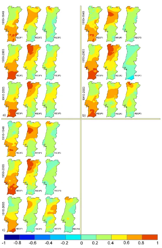
CONFIDENCE LEVEL RESULTING FROM THE PCA APPLIED TO THE SPI COMPUTED ON DIFFERENT TIME SCALES (ROWS) USING OBSERVATIONS (193 STATIONS) AND PT02 AND GPCC DATA SETS (COLUMNS).ADAPTED FROM RAZIEI ET AL (2015). ... 35 FIGURE 2-5VARIMAX ROTATED LOADINGS (REOFS) RELATIVE TO THE SPI ON A)3-, B)6-, C)12- AND D)24-MONTH TIME

SCALE, COMPUTED USING OBSERVATIONS (193 STATIONS), AND PT02 AND GPCC PRECIPITATION DATA SETS. ... 38 FIGURE 2-6VARIMAX ROTATED LOADINGS (REOFS) RELATIVE TO THE SPI ON A)3-, B)12-, AND C)24-MONTH TIME SCALE,

COMPUTED USING OBSERVATIONS FROM 144 STATIONS FOR 1910–1949,1950–2003 AND 1910–2003 TIME WINDOWS. ... 43 FIGURE 2-7ROTATED PRINCIPAL COMPONENT SCORE TIME SERIES (RPCS) ASSOCIATED WITH THE REOFS ILLUSTRATED IN

FIGURE 2-5.ROWS FROM TOP TO BOTTOM REFER TO THE SPI-3,SPI-6,SPI-12 AND SPI-24, RESPECTIVELY.

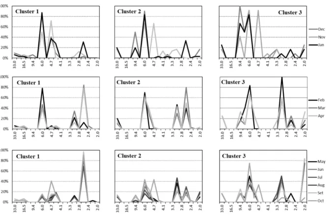
HORIZONTAL DOTTED LINE IS THE ZERO-LINE. ... 44 FIGURE 2-8THE MOST FREQUENT DROUGHT CLASS BY MONTH IN PORTUGAL (ALL), CLUSTER 1, CLUSTER 2 AND CLUSTER 3(1

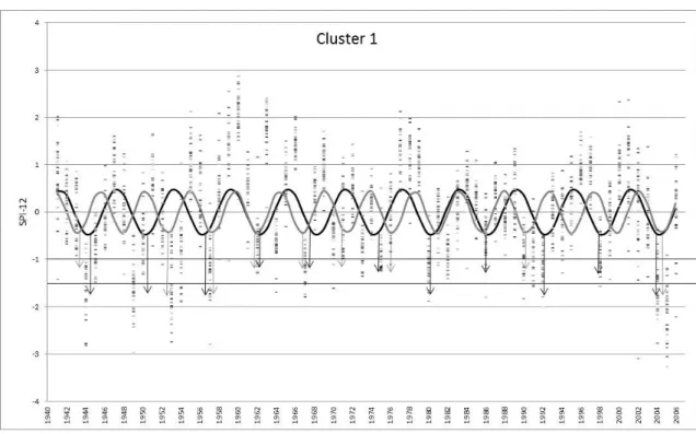
– NON DROUGHT,2– NEAR NORMAL,3– MODERATE,4– SEVERE,5– EXTREME) USING THE SPI WITH THE 12 MONTH TIME SCALE.CONSEQUTIVE DRY EVENTS WITH DROUGHT CLASS =>3 ARE HIGHLIGHTED IN ORANGE AND CONSEQUTIVE DRY EVENTS WITH DROUGHT CLASS =>4 ARE HIGHLIGHTED IN RED... 47 FIGURE 2-9SPI-12DECEMBER VALUES FOR NORTHERN PORTUGAL (CLUSTER 1) AND THE WAVES OF PERIOD 4.7 YEARS (GREY

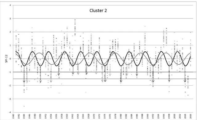
LINE) AND 6 YEARS (BLACK LINE).THE DOTS REPRESENT THE SPI-12 TIME SERIES FROM ALL LOCATIONS IN CLUSTER 1. ... 50 FIGURE 2-10SPI-12DECEMBER VALUES FOR CENTRAL/SOUTHERN PORTUGAL (CLUSTER 2) AND THE WAVES OF PERIOD 4.7

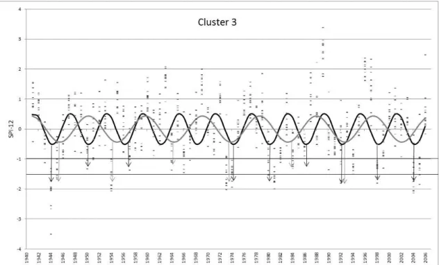
YEARS (GREY LINE) AND 6 YEARS (BLACK LINE).THE DOTS REPRESENT THE SPI-12 TIME SERIES FROM ALL LOCATIONS IN CLUSTER 2. ... 51 FIGURE 2-11SPI-12DECEMBER VALUES FOR SOUTHERN PORTUGAL (CLUSTER 3)+ WAVES OF PERIOD 6(BLACK LINE) AND

9.4 YEARS (GREY LINE).THE DOTS REPRESENT THE SPI-12 TIME SERIES FROM ALL LOCATIONS IN CLUSTER 3. ... 52 FIGURE 2-12FREQUENCY OF SIGNIFICANT CYCLES RELATIVE TO EACH CLUSTER PER PERIOD CYCLE, GATHERED IN THREE

GROUPS:NOVEMBER,DECEMBER AND JANUARY (WET SEASON);FEBRUARY,MARCH AND APRIL (TRANSITION MONTHS); AND MAY–SEPTEMBER (DRY SEASON) ... 55

(25)

xxii

FIGURE 3-1 A)LOCATION OF THE METEOROLOGICAL STATIONS USED FOR THE SPI ANALYSIS, WITH THE ARROW REPRESENTING SIGNIFICANT TRENDS FOR THE INCREASE OF ANNUAL PRECIPITATION AMOUNT; B)DISTRIBUTION OF THE 20TH

REANALYSIS GRIDPOINTS AND, UDOMETRIC STATIONS AND CRU GRIDPOINTS USED FOR COMPUTING THE PDSI. ... 67 FIGURE 3-2ANNUAL PRECIPITATION (OCTOBER TO SEPTEMBER) IN 4 OR 3 TIME SUB-PERIODS ACCORDING TO THE LENGTH OF DATA RECORDS ... 69 FIGURE 3-3GAMMA PROBABILITY DISTRIBUTION FUNCTIONS (ON LEFT) AND CUMULATIVE DISTRIBUTION FUNCTIONS (ON

RIGHT) OF ANNUAL PRECIPITATION CUMULATED FROM OCTOBER TO SEPTEMBER FOR THE FULL DATA RECORDS AND THE FOUR SUB-PERIODS FOR MONTALEGRE,PORTO,LISBOA AND ÉVORA.THE HISTOGRAM OF THE PRECIPITATION

FREQUENCIES FOR THE FULL PERIOD IS ALSO SHOWN. ... 76 FIGURE 3-4ZOOM ON THE LOWER TAIL OF THE GAMMA CUMULATIVE DISTRIBUTION FUNCTIONS OF MONTALEGRE,PORTO,

LISBOA AND ÉVORA FOR THE FULL PERIOD OF RECORDS AND FOUR SUB-PERIODS WITH IDENTIFICATION OF THE RELATED SPI-12 THRESHOLDS OF MODERATE, SEVERE AND EXTREME DROUGHT CATEGORIES RELATIVE TO THE 12-MONTH PRECIPITATION FROM OCTOBER TO SEPTEMBER. ... 78 FIGURE 3-5SPI-12 AT MONTALEGRE,PORTO,ÉVORA AND LISBOA COMPUTED FOR THE FULL DATA PERIOD AND FOR THE SUB -PERIODS. ... 80 FIGURE 3-6COMPARISON OF THE COUNT OF OCCURRENCES IN EACH CLASS OF PDSI AND SPI-9 COMPUTED REANALYSIS AND

OBSERVATIONS (EXT.DRY:EXTREME DROUGHTS;SEV.DRY:SEVERE DROUGHTS;MOD.DRY:MODERATE DROUGHTS; MILD DRY:MILD DROUGHTS;INCIP.DRY:INCIPIENT DROUGHT;INCIP.WET:INCIPIENTLY WET;MILD WET:MILDLY WET;MOD.WET:MODERATELY WET;VERY WET:VERY WET;EXT.WET:EXTREMELY WET). ... 87 FIGURE 4-1CLIMATIC ARIDITY MAP OF INNER MONGOLIA AND SPATIAL DISTRIBUTION OF THE WEATHER STATIONS.IN RED ARE THE STATION THAT WERE NOT USED FOR TREND ANALYSIS. ... 101 FIGURE 4-2ANNUAL PM-ETO(MM) IN INNER MONGOLIA ... 104

FIGURE 4-3SPATIAL DISTRIBUTION OF THE STATISTICAL PERFORMANCE INDICATORS COMPARING ETO PMTWITH PM-ETO: A)

REGRESSION COEFFICIENT, B0, B) COEFFICIENT OF DETERMINATION, C) ROOT MEAN SQUARE ERROR, AND D) MODELING EFFICIENCY (ARIDITY INCREASES FROM EAST TO WEST,FIGURE 4-1). ... 112 FIGURE 4-4SPATIAL PATTERNS OF THE OPTIMAL KRS (℃-0.5) OVER INNER MONGOLIA FOR:(A)PMT AND (B)HS METHODS

(ARIDITY INCREASES FROM EAST TO WEST,FIGURE 4-1). ... 113 FIGURE 4-5SPATIAL DISTRIBUTION OF STATISTICAL PERFORMANCE INDICATORS COMPARING ETO HS WITH PM-ETO: A)

REGRESSION COEFFICIENT, B) COEFFICIENT OF DETERMINATION, C) ROOT MEAN SQUARE ERROR, AND D) MODELING EFFICIENCY (ARIDITY INCREASES FROM EAST TO WEST AS PER FIGURE 4-1). ... 115 FIGURE 4-6SPATIAL DISTRIBUTION OF SEASONAL ETO COMPUTED WITH FAO-PM(A-D),PMT(E-H) AND HS(I-L). ... 117

FIGURE 4-7SPATIAL DISTRIBUTION OF THE ROTATED PC-SCORES OF ETO VARIABLES. ... 119

FIGURE 4-8SPATIAL DISTRIBUTION OF RMSE RESULTS WHEN COMPARING PMT AND HS METHODS THROUGHOUT INNER MONGOLIA. ... 120 FIGURE 4-9SPATIAL DISTRIBUTION OF DETERMINISTIC LINEAR TRENDS OF ANNUAL ETO IN INNER MONGOLIA. ... 124

FIGURE 4-10SPATIAL DISTRIBUTION OF ANNUAL TRENDS OF THE CLIMATIC VARIABLES IN INNER MONGOLIA: A) MAXIMUM TEMPERATURE (TMAX), B) MINIMUM TEMPERATURE (TMIN), C) SUNSHINE DURATION (SD), D) RELATIVE HUMIDITY (RH)

(26)

xxiii

FIGURE 4-11SPATIAL DISTRIBUTION OF THE SEASONAL TREND ANALYSIS APPLIED TO PM-ETO: A)MAM(MARCH,APRIL AND

MAY), B)JJA(JUNE,JULY AND AUGUST), C)SON(SEPTEMBER,OCTOBER AND NOVEMBER), D)DJF(DECEMBER, JANUARY AND FEBRUARY) AND E) ANNUAL. ... 134 FIGURE 4-12SPATIAL DISTRIBUTION OF THE TREND ANALYSIS OF SEASONAL CLIMATIC VARIABLES IN INNER MONGOLIA ... 135 FIGURE 5-1SPATIAL DISTRIBUTION OF THE REANALYSIS GRID POINTS (AT EACH 0.5°) AND THE 130PORTUGUESE AND SPANISH

WEATHER STATIONS OVER THE IBERIAN PENINSULA ... 146 FIGURE 5-2FLOW CHART OF THE PROCEDURE TO ESTIMATE PM-ETO FROM REANALYSIS DATA AND COMPARING WITH

OBSERVATIONS. ... 148 FIGURE 5-3EXAMPLES OF LINEAR REGRESSIONS BETWEEN ETO COMPUTED WITH MONTHLY AVERAGES OF THE WEATHER

VARIABLES AND DAILY ETO CUMULATED TO THE MONTH WHEN COMPUTED WITH DAILY VALUES OF THE SAME VARIABLES

(ETO D).THE MAP IDENTIFIES THE LOCATIONS OF THE SELECTED WEATHER STATIONS. ... 155

FIGURE 5-4EXAMPLES OF LINEAR REGRESSIONS OF ETOREAN RELATIVE TO ETOOBSUSING BOTH THE ORDINARY LEAST SQUARES AND THE REGRESSION FORCED TO THE ORIGIN.THE MAP IDENTIFIES THE LOCATIONS OF THE SELECTED WEATHER STATIONS. ... 157 FIGURE 5-5SPATIAL DISTRIBUTION OF THE STATISTICAL INDICATORS MEASURING THE PERFORMANCE OF ETO ESTIMATION WITH

BLENDED REANALYSIS DATA SETS. ... 159 FIGURE 5-6EXAMPLES OF LINEAR REGRESSIONS OF RSREAN OVER RSOBS USING BOTH THE ORDINARY LEAST SQUARES AND THE

REGRESSION FORCED TO THE ORIGIN.THE MAP IDENTIFIES THE LOCATIONS OF THE SELECTED WEATHER STATIONS. .. 164 FIGURE 5-7EXAMPLES OF LINEAR REGRESSIONS OF TMAXREAN OVER TMAXOBS AND TMINREAN RELATIVE TO TMIN OBS USING BOTH

THE ORDINARY LEAST SQUARES AND THE REGRESSION FORCED TO THE ORIGIN.THE MAP IDENTIFIES THE LOCATIONS OF THE SELECTED WEATHER STATIONS ... 166 FIGURE 5-8SPATIAL DISTRIBUTION OF STATISTICS MEASURING THE ASSOCIATION BETWEEN OBSERVED AND BLENDED

REANALYSIS DATA SETS OVER THE IBERIA FOR SHORTWAVE RADIATION (RS) AND MAXIMUM AND MINIMUM

TEMPERATURE (TMAX AND TMIN) ... 167

FIGURE 5-9EXAMPLES OF LINEAR REGRESSIONS OF RHREAN OVER RHOBS USING BOTH THE ORDINARY LEAST SQUARES AND THE REGRESSION FORCED TO THE ORIGIN.LOCATIONS ARE THE SAME AS FOR MINIMUM TEMPERATURE. ... 169 FIGURE 5-10EXAMPLES OF LINEAR REGRESSIONS OF WSREAN OVER WSOBS USING BOTH THE ORDINARY LEAST SQUARES AND

THE REGRESSION FORCED TO THE ORIGIN.THE MAP IDENTIFIES THE LOCATIONS OF THE SELECTED WEATHER STATIONS. ... 170 FIGURE 5-11SPATIAL DISTRIBUTION OF STATISTICS MEASURING THE ASSOCIATION BETWEEN OBSERVED AND BLENDED

REANALYSIS DATA SETS OVER THE IBERIA FOR RELATIVE HUMIDITY (RH) AND WIND SPEED (WS). ... 171 FIGURE 5-12SPATIAL DISTRIBUTION OF THE ERA-INTERIM REANALYSIS GRID POINTS (AT EACH 0.75°) IN CONTINENTAL

PORTUGAL AND LOCATION OF THE 24 WEATHER STATIONS USED IN THE CURRENT ANALYSIS. ... 177 FIGURE 5-13CROSS-VALIDATION DAILY ETOREAN MEAN PERFORMANCE INDICATORS RELATIVE TO THE (A) ADDITIVE BIAS

CORRECTION AND (B) MULTIPLE REGRESSION USING THE DIFFERENT AGGREGATION PERIODS MONTHLY (Δ), QUARTERLY (•), AND ENTIRE PERIOD (*) ... 182

(27)

xxiv

FIGURE 5-14FREQUENCY (%) DISTRIBUTION OF THE STATISTICAL INDICATORS MEASURING THE PERFORMANCE OF ETO

ESTIMATION USING UNCORRECTED REANALYSIS DATA, ADDITIVE BIAS CORRECTION AND MULTIPLE REGRESSION WITH QUARTERLY AGGREGATION ... 184 FIGURE 6-1MAP WITH THE LOCATION OF THE REANALYSIS GRIDPOINTS USED AND THE WEATHER STATIONS CLASSIFIED BY

ARIDITY (ON THE LEFT) WITH THE COORDINATES OF THE WEATHER STATIONS THE RESPECTIVE ARIDITY INDEX ON THE RIGHT.HIGHLIGHTED LOCATIONS WERE SELECTED TO DEPICT THE BEHAVIOUR OF THE DROUGHT INDICES FOR DIFFERENT CLIMATES. ... 197 FIGURE 6-2INTRAANNUAL VARIABILITY OF PRECIPITATION,REFERENCE EVAPOTRANSPIRATION (PM-ETO) AND POTENTIAL

EVAPOTRANSPIRATION (PET), CONSIDERING MONTHLY MEANS RELATIVE TO THE PERIOD 1941-2006 FOR 6 SELECTED STATIONS AND ORDERED BY ARIDITY, FROM DRY-SUB-HUMID TO HUMID. ... 199 FIGURE 6-3EVAPORATION COEFFICIENT (KE) COMPUTED FOR ALL 26 LOCATIONS, FROM THE HUMID STATIONS ( ) TO THE

DRY SUB-HUMID STATIONS ( ) CONSIDERING A LOAM SOIL. ... 207 FIGURE 6-4INTRAANNUAL VARIABILITY OF THE WATER BALANCE INPUTS (ETC AND PET) AND OUTPUTS: ACTUAL

EVAPOTRANSPIRATION (ETACT) AND RUNOFF PLUS DEEP PERCOLATION (RO+DP), COMPUTED FOR THE PDSI( ) AND

MEDPDSI( ) FOR SIX SELECTED LOCATIONS. ... 210 FIGURE 6-5COMPARISON OF ACTUAL EVAPOTRANSPIRATION (ETACT) COMPUTED WITH PDSI,MEDPDSI, FOR THE PERIOD

1994-2006. ... 213 FIGURE 6-6COMPARISON OF THE MOISTURE ANOMALY (ZINDEX) INDEX COMPUTED FOR THE PDSI AND THE MEDPDSI FOR

SELECTED STATIONS. ... 218 FIGURE 6-7ACCUMULATED ZINDEX OVER THE DRIEST AND WETTEST PERIODS FOR THE MEDPDSI( ) AND PDSI( ) FOR

SELECTED STATIONS ... 220 FIGURE 6-8TIME VARIABILITY OF THE PDSI(RED) AND MEDPDSI(BLACK) FOR SELECTED STATIONS FOR THE PERIOD

1948-2006(ON THE LEFT) AND A TIME WINDOW WITH THE DROUGHTS FROM 1990-2006(ON THE RIGHT).THE SEVERE DROUGHT THRESHOLD IS DEPICTED BY ( ) AND EXTREME DROUGHT BY ( ). ... 223 FIGURE 6-9FREQUENCY OF EVENTS IN EACH DRY AND WET CLASS OF THE MEDPDSI AND PDSI FOR SELECTED STATIONS ... 225 FIGURE 6-10COMPARING SPI-9 WITH MEDPDSI WITH THE RESPECTIVE LINEAR REGRESSION AND R2_{... 227} FIGURE 6-11TIME VARIABILITY OF THE SPI-9(RED) AND MEDPDSI(BLACK) FOR SELECTED STATIONS FOR THE PERIOD

1948-2006(ON THE LEFT) AND A TIME WINDOW WITH THE DROUGHTS FROM 1990-2006(ON THE RIGHT).THE SEVERE DROUGHT THRESHOLD IS DEPICTED BY ( ) AND EXTREME DROUGHT BY ( ).THE LEFT YY AXIS CORRESPOND TO THE SEVERITY SCALE OF THE MEDPDSI AND THE YY AXIS THE RIGHT FOR THE SPI-9 SCALE. ... 229

(28)

xxv

List of Tables

TABLE 1-1LIST WITH SELECTED DROUGHT INDICES AS EXAMPLES OF THE DIVERSITY OF INDICES AND INDICATORS AVAILABLE FOR DROUGHT MONITORING.PRE IS PRECIPITATION;ET IS EVAPOTRANSPIRATION;SWC IS WATER HOLDING CAPACITY;T IS TEMPERATURE;WS IS WIND SPEED; ... 9 TABLE 1-2PERSONAL CONTRIBUTION TO THE PEER-REVIEWED PAPERS ADAPTED IN CHAPTERS 2 TO 6. ... 17 TABLE 2-1SPI DROUGHT CLASS CLASSIFICATION (MCKEE ET AL.(1993)) ... 29 TABLE 2-2PERCENTAGE OF THE TOTAL VARIANCE EXPLAINED BY THE UN-ROTATED (UR) AND VARIMAX ROTATED (VR)

LOADINGS OF THE SPI ON DIFFERENT TIME SCALES COMPUTED USING OBSERVATIONS AND GRIDDED PT02 AND GPCC DATA SETS.UNITS ARE % ... 36 TABLE 2-3INTER-COMPARISON OF THE THREE USED DATA SETS BY RELATING THEIR ROTATED LOADINGS ASSOCIATED WITH

DIFFERENT SPI TIME SCALES THROUGH CONGRUENCE COEFFICIENTS. ... 40 TABLE 2-4PERCENTAGE OF THE TOTAL VARIANCE EXPLAINED BY THE UN-ROTATED (UR) AND VARIMAX ROTATED (VR)

LOADINGS OF THE SPI-3,SPI-12 AND SPI-24 COMPUTED USING 144 OBSERVATIONS DATA SET FOR THREE DIFFERENT TIME SECTIONS.UNITS ARE IN %. ... 41 TABLE 2-5CORRELATION COEFFICIENTS BETWEEN THE RPCS FOR OBSERVATIONS (OBS) AND PT02 AND GPCC GRIDDED

DATA SETS.CORRELATION COEFFICIENTS BETWEEN RPCS ASSOCIATED WITH THE SAME SUB-REGIONS ARE IN BOLD .... 45 TABLE 2-6RESULTS OF THE SEN SLOPE ESTIMATES AND THE MANN-KENDALL TREND TEST (IN PARENTHESIS) APPLIED TO THE

ANNUAL AVERAGE OF RPC SCORES RELATIVE TO SPI-12 AND SPI-24 OF PT02.THE STATISTICALLY SIGNIFICANT VALUES AT 0.05 SIGNIFICANT LEVEL ARE IN BOLD ... 46 TABLE 2-7THE COUNTS PER CYCLE AND PER CLUSTER AND ITS FREQUENCY (%) RELATIVE TO THE NUMBER OF SERIES INCLUDED IN EACH CLUSTER (JUST THE SIGNIFICANT CYCLES OF THE PERIODOGRAMS). ... 49 TABLE 3-1LOCATION OF THE METEOROLOGICAL STATIONS, DATE OF RECORDS, RECORD LENGTH AND DURATION OF THE FIRST

SUB-PERIOD USED FOR THE SPI ANALYSIS. ... 68 TABLE 3-2UPPER THRESHOLDS OF SPI DROUGHT CATEGORIES AND RESPECTIVE CUMULATIVE PROBABILITIES ... 71 TABLE 3-3MEAN, STANDARD DEVIATION AND COEFFICIENT OF ASYMMETRY ESTIMATED FROM THE GAMMA DISTRIBUTION

FITTED TO THE CUMULATED PRECIPITATION (OCTOBER TO SEPTEMBER) FOR THE FULL TIME PERIOD AND THE

CONSIDERED SUB-PERIODS ... 74 TABLE 3-4PRECIPITATION THRESHOLDS (MM) CORRESPONDING TO SPI-12=0(MEDIAN),SPI-12=-1,-1.5,-2(MODERATE,

SEVERE AND EXTREME DROUGHT CATEGORIES) COMPUTED FOR SEPTEMBER WITH THE FULL RECORDS AND RESPECTIVE SUB-PERIODS FOR ALL WEATHER STATIONS. ... 79 TABLE 3-5COMPARING THE PERCENTAGE OF TIME IN MODERATE, SEVERE AND EXTREME DROUGHT/WETNESS CATEGORIES FOR

THE FULL PERIOD (FULL) OF RECORDS AND THE VARIOUS SUB-PERIODS (SUB);MONT. IS MONTALEGRE;EXTR+S IS EXTREME PLUS SEVERE AND MODER IS MODERATE ... 81 TABLE 3-6COMPARISON OF MEAN (Μ) AND STANDARD DEVIATION (Σ2) OF REANALYSIS PRECIPITATION AND PM-ETO IN EACH

(29)

xxvi

TABLE 3-7PERFORMANCE INDICATORS RELATIVE TO THE COMPARISON BETWEEN PREREAN AND PM-ETO REANAGAINST PRE OBS AND PM-ETO-OBS ... 85

TABLE 3-8COUNT OF OCCURRENCES IN EACH CLASS OF PDSI AND SPI-9 USING DIFFERENT CALIBRATION PERIODS FOR GRID2 AND GRID3 ... 89 TABLE 4-1COORDINATES AND ARIDITY INDEX (AI) OF THE 50 WEATHER STATIONS OF INNER MONGOLIA USED IN THE

CURRENT STUDY. ... 102 TABLE 4-2.CALIBRATED KRS COEFFICIENT AND STATISTICAL PERFORMANCE INDICATORS WHEN COMPARING THE ETO PMT WITH

THE PM-ETO. ... 111

TABLE 4-3CALIBRATED KRS COEFFICIENT AND STATISTICAL PERFORMANCE INDICATORS WHEN COMPARING THE ETO HS WITH THE PM-ETO. ... 114

TABLE 4-4EXPLAINED VARIANCES OF THE ROTATED PRINCIPAL COMPONENTS CORRESPONDING TO THE THREE SETS OF ETO

VARIABLES. ... 118 TABLE 4-5COMPARING THE PERFORMANCES OF HS AND PMT METHODS (HIGHLIGHTED CELLS REFER TO BETTER RESULTS).

... 121 TABLE 4-6TRENDS (MM YR-1) FOR PM-ETO COMPUTED WITH FULL DATA SETS USING BOTH THE MMK TEST ASSOCIATED

WITH THE SEN SLOPE AND THE KPSS TEST ASSOCIATED WITH THE GLS LINEAR TREND.SIGNIFICANT RESULTS WERE ASSUMED FOR A CONﬁDENCE LEVEL OF 95%. ... 123 TABLE 4-7TRENDS IN ETO(MM YR-1) COMPUTED WITH TEMPERATURE METHODS,HS AND PMT USING BOTH THE MMK TEST

ASSOCIATED WITH THE SEN SLOPE AND THE KPSS TEST ASSOCIATED WITH THE GLS LINEAR TREND.SIGNIFICANT RESULTS WERE ASSUMED FOR A CONﬁDENCE LEVEL OF 95%.ALL COLUMNS ARE IN MM YR-1 ... 126 TABLE 4-8LINEAR TRENDS OF THE WEATHER VARIABLES MAXIMUM AND MINIMUM TEMPERATURE (TMAX AND TMIN,OC DECADE

-1_),_{SOLAR DURATION}_(SD,_{H DECADE}-1_),_{RELATIVE HUMIDITY}_(RH,_%_DECADE-1₎_{AND WIND SPEED}_(WS,_{M S}-1_DECADE-1_). THE CONFIDENCE LEVEL OF 95% WAS ASSUMED. ... 130 TABLE 5-1PERFORMANCE INDICATORS RELATIVE TO THE COMPARISON BETWEEN ETO COMPUTED WITH MONTHLY AVERAGES

OF THE WEATHER VARIABLES AND DAILY ETO CUMULATED TO THE MONTH (BOTH EXPRESSED IN MM D-1). ... 154

TABLE 5-2FREQUENCY (%) DISTRIBUTION OF THE PERFORMANCE INDICATORS COMPARING ETO COMPUTED WITH REANALYSIS

PRODUCTS WITH ETO COMPUTED FROM OBSERVED WEATHER DATA. ... 156

TABLE 5-3FREQUENCY (%) DISTRIBUTIONS OF THE PERFORMANCE INDICATORS FOR SHORTWAVE RADIATION (RS), MAXIMUM TEMPERATURE (TMAX) AND MINIMUM TEMPERATURE (TMIN) WHEN COMPARING REANALYSIS PRODUCTS WITH OBSERVED

VALUES ... 5-162 TABLE 5-4FREQUENCY (%) DISTRIBUTION OF THE PERFORMANCE INDICATORS FOR HUMIDITY (RH) AND WIND SPEED (WS),

WHEN COMPARING REANALYSIS PRODUCTS WITH OBSERVED VALUES. ... 5-173 TABLE 5-5COMPARING THE PERFORMANCE INDICATORS RELATIVE TO THE ESTIMATION OF ETO BY ERA-INTERIM,NCEP2 AND

BLENDED NCEP/NCARREANALYSIS FOR 15 WEATHER STATIONS IN THE IBERIAN PENINSULA.*UNITS IN MM D-1 ... 175 TABLE 5-6AVERAGE GOODNESS-OF-FIT INDICATORS RELATIVE TO THE ESTIMATION OF ETO AND THE WEATHER VARIABLES BY

THE NCEP-NCARREANALYSIS II PRODUCTS FOR THE PERIOD 1998-2008 AND 1998-2014 FOR 94SPANISH WEATHER STATIONS ... 176 TABLE 6-1CLASSIFICATION OF SEVERITY OF DROUGHT/WETNESS EVENTS OF THE PDSI ... 200

(30)

xxvii

TABLE 6-2WATER BALANCE POTENTIAL COEFFICIENTS (Α, Β, Δ, Γ) AND CLIMATIC CHARACTERISTIC (K) FOR FARO,ELVAS AND ALVALADE DO SADO ... 215 TABLE 6-3AVERAGE FREQUENCY (%) OF DROUGHT/WET CLASSED OF THE MEDPDSI AND PDSI GROUPED BY ARIDITY FOR ALL 26 WEATHER STATIONS ... 226

(31)

1

Chapter 1

Introduction

Water is a finite resource essential for all socio-economic development and for maintenance of ecosystems (Pereira et al. 2009). Human growth and development is responsible for the increase pressure on water resources. Moreover, the increased variability of climate, which is becoming less predictable, due to climate change, with higher temperatures and a larger variability in precipitation and temperature ranges, extreme events such as floods, heat waves, droughts, will become more frequent and intense. Thus, a better water management is a key for the adaptation of society and ecosystems to climate change (UNEP 2006; Pereira 2017).

Irrigated agriculture is still the largest user of freshwater, accounting for 46% of the Europe’s total water withdrawal (European Environment Agency 2018). The effects of climate change, combined with the increasing demand for food supply, makes irrigated agriculture quite vulnerable to the future climate conditions. Thus, this reality, combined with the large uptake of water by irrigated agriculture exacerbates the need to make irrigated agriculture more efficient, regarding water use, which can be achieved by adopting improved irrigation methods and less consumptive crops. This would allow for an increase in irrigation efficiency and the use of other sources of water for irrigation, like wastewater or other forms of low quality waters that cannot be used for other purposes must be considered (Pereira et al 2009). Increasing water demand is due to a variety of factors: expansion of irrigation in agriculture, worlds population increase, changes in consumption patterns and living habits (Vörösmarty et al. 2000). All these factors combined with an increased uncertainty in climate, is leading towards an intensification of water scarcity, i.e., when the available water in a determined moment is not enough to meet local and global demands of water, endangering the sustainable development of human society.

Water scarcity occurs when there is a geographic and temporal negative balance between fresh water requirements and fresh water availability (Mekonnen and Hoekstra 2016).

(32)

2

Furthermore, water scarcity is not only due to physical shortage of quality freshwater but also due to the failure of regular supply of freshwater or because of inadequate infrastructure conditions. While reviewing the diversity of water scarcity definitions and indicators, Rijsberman (2006) defined water scarcity as lack of accessibility to safe and affordable water to satisfy the needs of a person. When this affects more people on a larger scale, that area is considered water scarce. Using the definition by Hoekstra et al. (2012) and Mekonnen and Hoekstra (2016) of blue water (fresh surface water and groundwater) scarcity, these authors found consistent yearly blue water scarcity worldwide, most noticeable in forest areas such as the Amazon or Congo basins. Furthermore, water scarcity was observed in southern and Western Europe, and was more frequent and intense in the summer months (July, August and September) but also ocurred throughout the rest of year, being less severe and spatially spread in the months from January to March. Hoekstra et al. (2012) and Mekonnen and Hoekstra (2016) concluded that 71% of the global population suffer from moderate to severe water scarcity every year.

Pereira et al. (2009) considered four different xeric regimes that may cause water scarcity, which may be natural or anthropogenic or may be permanent or temporary. Those regimes are:

(1) Aridity is a permanent and natural phenomenon of a region characterized by extremely low annual average rainfall and aggravated by high spatial and temporal variability in its occurrence, which has significant implications for the maintenance of ecosystems and limits any human activity. Aridity is usually studied as the ratio between precipitation and potential evapotranspiration, computed using the Thornthwaite equation (Thornthwaite 1948);

(2) Droughts, are also natural phenomenons, althought temporary, and are extreme events characterized by persistently below-average rainfall, often with uncertain duration and severity, and their occurrence is very difficult to predict. Droughts consequences results in a temporary decrease in the availability of water for their various uses. It is the uncertainty associated with the droughts that make this phenomenon extraordinarily complicated to manage;

(3) Desertification is permanent and man-induced, and develops over several generations, in which the imbalance in water availability is due to the impoverishment of the land (for example through soil erosion and salinization),

(33)

3

unsustainable use, on groundwater exploration, increasing frequency of rapid floods, degradation of riparian systems and the sustainability of ecosystems in general. Desertification effects are more noticeable in arid, semi-arid and sub-humid climates and are aggravated by the occurrence of droughts.

(4) Water shortage is not only related to the amount of water available to satisfy demand, but also due to the quality of water, which, sometimes, does not have enough quality to be used, for example, for domestic consumption or industrial applications. Water shortages are of anthropogenic, albeit temporary, origin and consist of overexploitation and quality degradation of surface or underground water resources, incorrect land use, and changes in ecosystem support capacity.

1.1

Droughts

Droughts are stochastic, natural phenomenons that stem from persistent conditions of low precipitation amounts, below average, for a specific period in a region. (Wilhite 2000; Zargar et al. 2011). From a physical standpoint, drought is a reduction, of the water balance terms, for a given location and period that affects soil water content, deep percolation and surface runoff (Pires 2015). Moreover, droughts are common to all types of climate and can occur in high or low rainfall areas and are spatially and context dependent (Quiring 2009). Droughts occurrence, especially in vulnerable regions, such as poor and arid countries can result in significant humanitarian problems. Being a climate event of slow-onset, drought effects accumulate over time, making the determination of the start and end of a dry spell very difficult to assess and thus hindering policy making regarding drought risk management (Wilhite and Glantz 1985). It is also difficult to assess drought severity and its impacts, because it depends not only on the duration of drought but of its intensity and the spatial extent of a dry spell, but also depend upon the local water demand, the local water management policies and the resilience of the ecosystems or human activities to droughts.

Drought impacts are felt on a multiplicity of areas (agriculture, environment, meteorology, hydrology, geology). Reported impacts of droughts are always associated with losses in agriculture and livestock farming being the most affected sector, but drought are also related with forest fires, freshwater supply and ecosystems, water quality and droughts impact significantly the energy, industry and tourism sectors (Stahl et al. 2016). The extreme drought of 2005-2006 that affected most of Iberian Peninsula had

(34)

4

significant impacts on cereal yield on the European Union, with an estimated reduction of 10% of cereal yields (UNEP 2006). Because drought affect most of human activities and ecosystems it does not have a consensual definition, since it depends on the point of view of the stakeholder and affected sector (Pereira et al. 2009; Mishra and Singh 2010). The World Meteorological Organization (WMO) defines drought as a normal and recurring event of the climate (Monacelli et al. 2005). It differs from aridity, in which very low precipitations are characteristic of the climate of the region. Drought should be relative to the average conditions of the balance between precipitation and evapotranspiration in a given area. Dracup et al. (1980) and Tate and Gustard (2000) provided a review of the many drought definitions. Moving from a conceptual definition to an operational one, Wilhite and Glantz (1985) distinguishes four types of drought: meteorological, agricultural, hydrologic, and socio-economic. This distinction of drought types is associated with a temporal evolution of the impacts, which is due primarily by the deficiencies in precipitation, called meteorological drought. Then the agricultural drought is felt, through the loss of moisture in the soil and then hydrological drought is noticed by the reduction of river flows and water storage in aquifers. When the reduction of available freshwater water starts to affect human activities and consumption it is considered that a socio-economic drought is occurring. Pereira et al (2009) defined drought as a natural temporary imbalance of water availability, consisting of a persistent lower-than-average precipitation, of uncertain frequency, duration and severity, of unpredictable or difficult to predict occurrence, resulting in diminished water resources availability and carrying capacity of the ecosystems. This definition provided a cohesive and multidisciplinary view of drought origins, its characteristics and potential impacts and is used throughout this Thesis.

The effects of drought will be felt first in agriculture, since there is less available water in the soil, only later the hydrological drought is felt, because the decrease in percolation and runoff continues over time, which results in a reduction of the recharge of aquifers and in surface water flows. All these constraints will have an impact on socio-economic activities, starting with agriculture, industry and reducing water availability for domestic consumption. These categories may be described in detail:

(1) Meteorological drought is characterized based upon the duration of the dry period and the degree of dryness (taking into account normal conditions). This type of

(35)

5

drought has to be addressed to the scale of the region since there is a high spatial variability of the precipitation that results from the atmospheric conditions. (2) Agricultural drought is fundamentally caused by precipitation deficits, which

affect the development of agricultural or forestry crops. This type of drought will depend upon the type of crop considered, that is, on the biological characteristics of the crop, and on the growth stage of the crop when drought settles. This category is ambiguous since the scarcity of water for agriculture is not only the result of deficit amounts of precipitation, but also due to a lack of adequate water and drought risk management in the region. This can occur either, because of an unsustainable increase of the agricultural area or because of the adoption of crops which are more water demanding, or simply by the lag between the precipitation regimes and the stages of growth of the crop.

(3) The hydrological drought is associated to the effects caused by the periods of lack of precipitation in the reduction of river flows, groundwater reservoirs, and storage in lakes, for example. This type of drought has to be considered at the level of the river basin. Changes to land use, such as dam construction, deforestation, and any type of soil degradation have significant consequences at the river basin level that may accentuate drought problems.

(4) Socioeconomic droughts arise when the lack of water begins to affect the general population and there is not enough water supply to fulfill all the demands. This type of drought relates more to an economic issue of supply and demand rather than with unfavorable climatic conditions. Climate change combined with increase in water consumption and lack of adequate management policies are exacerbating socioeconomic droughts.

1.1.1 Drought indicators and indices

Drought indices are numerical representations of drought (WMO and GWP 2016), and measure the various characteristics of drought, namely: duration, magnitude, intensity and spatial extent (Mishra and Singh 2010). The duration of a drought is expressed in years, months or weeks and is given by the period in which a series is below a pre-determined threshold. The magnitude of a drought is given by the sum of the drought index values for all the months within a dry event. The intensity is calculated from the ratio between magnitude and duration, and spatial extent is the area affected by a drought spell. Another usual term used to characterize droughts is severity, which is normally

(36)

6

associated with the degree of precipitation or moisture deficit, i.e., the numerical value of the drought index in a given moment in time.

Drought indices are tools used for measuring different events and conditions, since they can reflect climate dryness anomalies, when using precipitation based indices, or may be useful to quantify impacts on agricultural and hydrological systems by analyzing anomalies of soil moisture or of reservoir levels (Zargar et al. 2011). These indices are based upon inputs, which are climatic or hydrometeorological variables, and may be called drought indicators. These indicators can be precipitation, temperature, evapotranspiration, soil moisture, streamflow, groundwater or reservoir levels and even snowpack, or can be based upon combinations of these variables. The selection of what drought indicators to use depend upon the drought index and the types of drought the index aims at measuring (Zargar et al. 2011; WMO and GWP 2016).

Drought indices often result from a combination of these indicators or climatological variables. The essential variable used to compute meteorological drought indices is precipitation. Nevertheless evapotranspiration has been recognized as an equally important variable, measuring evaporative demand and was incorporated recently in drought indices, combining the contribution of precipitation and evapotranspiration: Such indices include the RDI (Reconnaissance Drought Index) (Tsakiris et al. 2007) or the Standardized Precipitation Evapotranspiration Index (SPEI) (Vicente-Serrano et al. 2010).

The impacts of temperature on droughts were given larger importance in recent years (Hobbins et al. 2017). However, the Palmer Drought Severity Index (PDSI) (Palmer 1965) was the first index to incorporate the effects of climate demand, by combining monthly precipitation and potential evapotranspiration, computed using the Thornthwaite equation (Thornthwaite 1948) in a water balance to obtain a moisture anomaly index, that after standardized could be used as a measurement of drought severity.

Although evapotranspiration (ET) is now considered an important climatic variable for drought monitoring, especially when temperature is increasing due to climate change, it is still a challenge to accurately incorporate this variable in drought indices. Evapotranspiration cannot be easily measured, like precipitation, and the best ET estimation is achieved using the FAO-PM equation (Allen et al. 1998), to compute the

(37)

7

reference evapotranspiration (PM-ETo). PM-ETo is the rate of evapotranspiration from a

hypothetical crop with an assumed fixed height (12 cm), surface resistance (70 s m−1) and albedo (0.23), closely resembling the evapotranspiration from an extensive surface of a disease-free green grass cover of uniform height, actively growing, completely shading the ground, and with adequate water and nutrient supply. Moreover, this equation provides appropriate estimates of the atmospheric evaporating capability and it can be applied to support irrigation management in agriculture, or to support drought management (e.g. Dai 2011). However, the computation of the PM-ETo equation requires

data relative to several climate variables: solar radiation (Rs) or sunshine duration, air

relative humidity (RH), maximum and minimum temperature (Tmax and Tmin) and wind

speed at 2 m height (u2), most of which are often not available. This increased the research

for alternative equations, capable of describing ET with lesser amount of variables and other data sources. Reanalysis products, remotely sensed data and forecast products, that have been improving in time, may provide such data with reasonable accuracy and with good spatial and temporal resolution, and thus may be useful for drought monitoring (Hobbins et al. 2017).

The use of temperature based equations to estimate ETo for drought indices is common.

Such equations are usually, the Hargreaves-Samani (HS) (Hargreaves and Samani 1985) or the Thornthwaite equation (Thornthwaite 1948). For example, the PDSI, SPEI and RDI were all introduced with potential evapotranspiration (PET) computed using the Thornthwaite equation. Nevertheless, since then, these indices have been tested with different ETo estimates, including the PM-ETo (e.g.: Dai, 2011; Vangelis et al., 2013;

Vicente-Serrano et al., 2015). The RDI was not significantly influenced by different ETo

estimations (Vangelis et al. 2013; Vicente-Serrano et al. 2015), whereas the SPEI showed a larger sensitivity to ETo computation methods (Vicente-Serrano et al. 2015). However,

studies analyzing the influence of the ETo equation on the PDSI showed contradictory

examples: while Sheffield et al. (2012) observed decreasing trends PDSI over large areas of the world, when the PDSI was computed using PM-ETo, which did not occur when the

PDSI was computed with PET. Both Dai (2011) and van der Schrier et al. (2011) did not find significant changes on the PDSI computed with both evapotranspiration equations. The results by Sheffield et al. (2012) are in agreement with other studies, which observed decreasing trends in reference evapotranspiration even though mean temperature is increasing (Espadafor et al. 2011; Vicente-Serrano et al. 2014). This review showed that

(38)

8

additional studies were required to further understand the differences between temperature based methods to compute ET and ET estimated with the full sets of climatological variables, such as the PM-ETo. Moreover, alternative sources of data to

estimate PM-ETo should also be tested so they can be used in drought indices to help

accurate drought characterization and drought monitoring. Thus, given the importance of evapotranspiration, an important part of this Thesis, focused on analyzing the accuracy of different ETo estimators, for different climates, in Chapter 4 and tested different data

sources, such as reanalysis products, to estimate reference evapotranspiration in Chapter 5. The conclusions from these Chapters were then useful for Chapters 3 and 6 in which the drought indices, using evapotranspiration as input, were computed with PM-ETo from

reanalysis data sets.

The ubiquity of drought in all types of climate and affecting almost all sectors of society and environment systems as led to the creation of many drought indices, with over 150 indices developed (Niemeyer 2008; Zargar et al. 2011; WMO and GWP 2016). Drought indices may be grouped according to the type of impacts they relate (Zargar et al. 2011). However, Niemeyer (2008) suggested two new categories: remotely-sensed drought indices that use data retrived from remote sensing and composite or combined drought indices that result from the combination of many drought indices and indicators to monitor drought and its impacts. Accordingly, WMO and GWP (2016) followed a similar taxonomy to group drought indices using the following classification: (a) meteorology, (b) soil moisture, (c) hydrology, (d) remote sensing and (e) composite or modelled. The most relevant drought indices for this Thesis were listed on Table 1-1. Thus, this Table included drought indices such as the Standardized Precipitation Index (McKee et al. 1995), the Palmer Drought Severity Index (PDSI) (Palmer 1965) and all its variations and drought indices, that despite not being used in the following chapters, are often studied and compared against the SPI and the PDSI, such as the abovementioned RDI and SPEI. Futhermore, in Table 1-1 some examples of drought indices based on remote sensing data and composite drought indices, were also included due to its relavance for drought monitoring. Similar reviews of drought indices are available in WMO and GWP (2016), Zargar et al. (2011). Table 1-1 differs from those studies regading the input requirements for the SPEI, RDI and PDSI and its variants, because it was considered that those indices require both precipitation and evapotranspiration data instead of precipitation and temperature data. As discussed above, those indices may be computed

(39)

9

using ET estimated based on temperature data only, however, is it preferable to use more realistic equations that consider the contribution of other variables such as radiation, wind speed or humidity rather than only temperature. The SPI characteristics and computational procedures were explained in detail in Chapters 2 and 3 and the PDSI and its variants including the MedPDSI were reviewed and described in Chapter 6.

Table 1-1 List with selected drought indices as examples of the diversity of indices and indicators available for drought monitoring. PRE is precipitation; ET is evapotranspiration; SWC is water holding capacity; T is temperature; WS is Wind speed;

Drought Index Input

data

Distinctive characteristics

Comprehensive drought indices Standardized Precipitation Index (SPI) (McKee et al. 1995)

PRE Standardized, multiscalar index. Quantifies deviations from normal precipitation conditions. SPI is computed by adjusting a probability distribution function to the precipitation cumulated over a given number of months denoted as time scale. Gamma and Pearson III distributions are most used.

Reconnaissance Drought Index (RDI) (Tsakiris et al. 2007)

PRE, ET Similar procedure to the SPI computation but considers the ratio PRE/ET to estimate departure from normal climate conditions.

Standardized Precipitation Evapotranspiration Index (SPEI) (Vicente-Serrano et al., 2010)

PRE, ET Same as the SPI but the relation between the climate variables is given by PRE-ET.

Palmer Drought Severity Index (PDSI) (Palmer 1965)

PRE, ET, SWC

Combines PRE and ET in a simple water balance. It was created to characterize and evaluate meteorological droughts by measuring the deviations between the observed and the expected precipitation, which are first transformed into an anomaly moisture index and then into a drought index, which is classified in terms of severity. Over the years many limitations regarding the PDSI computation have

(40)

10

been revealed (Alley 1985; Heddinghaus and Sabol 1991; Wells et al. 2004).

Self-calibrating PDSI (Sc-PDSI) (Wells et al. 2004)

PRE, ET, SWC

Based upon the PDSI. Changes all the empirical values of the original computation of the PDSI by values calculated dynamically based upon the characteristics present at each location. Allows for consistent results for different climates.

Zindex (Palmer 1965) PRE, ET,

SWC

An intermediary output of the PDSI. The Zindex was

considered a better indicator of short-term agriculture drought because it is sensible to variations in soil-moisture (Karl 1986).

Weighed PDSI (WPDSI) (Heddinghaus and Sabol 1991)

PRE, ET, SWC

The WPDSI removes the backtracking procedure proposed by Palmer in the PDSI to make it more adequate for real-time monitoring of drought. PHDI(Palmer 1965) Palmer

hydrological drought index

PRE, ET, SWC

Modification of the PDSI to account for longer-term dryness that will affect water storage, streamflow and groundwater.

standardized Palmer drought index (SPDI) (Ma et al. 2014)

PRE, ET, SWC

Multiscalar, standardized index based upon the moisture departure index obtained from the PDSI water balance.

MedPDSI (Pereira et al. 2007) and Chapter 6)

PRE, ET, SWC

Modifies the original PDSI soil water balance to one applied to an olive orchard, by estimating separately soil evaporation and transpiration of the olive crop adopting the dual crop coefficient approach and uses PM-ETo as the evapotranspiration input.

Modified PDSI (MPDSI) (Mo and Chelliah 2006)

Regional reanaysis data sets

Changed the PDSI original water balance to include reanalysis based data which are more accurate than those estimated by the original water balance. Such data included: potential evapotranspiration, evaporation, runoff, total soil moisture, and soil moisture change.

Standardized

Evapotranspiration Deficit

T, WS SEDI is a standardized multiscalar drought index, similar to SPEI but the P-ET component was