COLUMN GENERATION BASED ALGORITHMS FOR THE CAPACITATED MULTI-LAYER NETWORK DESIGN WITH UNSPLITTABLE DEMANDS

doi: 10.1590/0101-7438.2017.037.03.0545

COLUMN GENERATION BASED ALGORITHMS FOR THE CAPACITATED MULTI-LAYER NETWORK DESIGN WITH UNSPLITTABLE DEMANDS

Amal Benhamiche

, A. Ridha Mahjoub

,

Nancy Perrot

and Eduardo Uchoa

Received May 18, 2017 / Accepted October 23, 2017

ABSTRACT.We investigate a variant of the Multi-Layer Network Design problem where minimum cost capacities have to be installed upon a virtual layer in such a way that (i) a set of traffic demands can be routed AND (ii) each capacity (subband) is assigned a route in the physical layer. The traffic demands cannot be splitted along several paths (nor even several capacities installed on the same link), which makes the problem even more difficult. In this paper, we present new non-compact ILP formulations to model the problem and provide column generation procedures, based on different Dantzig-Wolfe decomposition schemes to solve it. More precisely, an arc-flow formulation is given for the problem and used to derive two different paths formulations: non-aggregated and aggregated. The former contains two families of path variables and requires a double column generation procedure to solve it, while the latter relies on a single path variable with a specific structure. These alternative modeling approaches induce two Branch-and-Price algorithms that allow to solve the problem efficiently for several classes of instances.

Keywords: multi-layer network design, linear programming, column generation, optical networks.

1 INTRODUCTION

1.1 Motivations

The emergence of multi-technology communication networks along with a continuous growth in traffic have driven many works in the field of multi-layer network optimization these past few years. In particular, recent trends observed in the optical fibers communications show up the so-called Orthogonal Frequency Division Multiplexing (OFDM) as a very promising technol-ogy, allowing for high and very high capacitated signals to reach long distances without being

*Corresponding author.

1Orange Labs, 92320 Chatillon, France. E-mails: amal.benhamiche@orange.com; nancy.perrot@orange.com 2Universit´e Paris-Dauphine PSL Research University, CNRS [7243], LAMSADE, 75016 Paris, France. E-mail: mahjoub@lamsade.dauphine.fr

regenerated. An OFDM-based network usually consists in a set of optical devices (ROADMs1) that are interconnected by optical channels. The OFDM infrastructure thus formed is called “virtual” layer, and lies on a “physical” layer that embeds and transports the signal carried out by the optical channels. The physical layer is composed by a set of transmission nodes, intercon-nected by optical fibers.

In fact, a specific feature of OFDM technology is precisely the opportunity to use only part of the optical channel in order to carry traffic from one point to another. An optical channel is then said to be divided into several units called “subbands”, each of which has a capacity (in terms of bandwidth) and a cost installation. The subbands can be set up and processed separately, which allows flexibility in the routing along with a more effective use of the whole capacity of the network. In this context, we consider theCapacitated Multi-Layer Network Design with Unsplit-table demands(CMLND-U) problem. Given a two-layer network and a set of traffic demands, this problem consists in installing minimum cost subbands on the upper (OFDM) layer so that each demand is routed along a unique “virtual” path (even using a unique subband on each link) in this layer, and each installed subband is in turn associated a “physical” path in the lower layer.

Example 1.1. Figure 1 shows a bilayer network. The virtual layer includes four ROADMs de-noted R1, R2, R3and R4, while physical layer contains six transmission nodes denoted T1to T6.

We can see that R1, R2, R3and R4are connected to T1, T2, T3and T4via

Optical-Electrical-Optical (OEO) interfaces. In addition, there exists a link between each pair of installed ROADMs. Remark that nodes R5and R6have not been represented in the figure, as they do not carry any

ROADM. Furthermore, three subbands are represented in the figure, respectively installed on the links(R1,R2),(R1,R3)and(R1,R4). The traffic using these virtual links is in fact transmitted

through paths made of optical fibers in the physical layer. Indeed, the link(R1,R2)is associated

with the path(T1,T2), while(R1,R3)is assigned the path(T1,T4), (T4,T3)and(R1,R4)is

physically routed by(T1,T6),(T6,T4).

It should be pointed out that there are two levels of routing in such networks. The traffic is routed using subbands installed on the virtual links, and the subbands themselves may be seen as demands for the physical layer. Thus, when given those two layers of network and a traffic matrix, one may determine the set of virtual links that will receive the subbands, and the set of physical links involved in the routing of those subbands, and establish the traffic commodities routing.

1.2 State-of-the-art

Actually, the problem of designing layered networks have been studied first by Dahl and Stoer in Dahl et al. (1999). The authors wish to set up a set of virtual links referred to as “pipes” on the physical layer. They propose an integer linear programming formulation based on cut constraints for the problem. They study the associated polytope and provide several classes of valid inequalities that define facets under some conditions which are described. They also provide a cutting planes based algorithm embedding their theoretical results.

Figure 1–Example of multilayer network.

Earlier works on this topic address the problem of designing virtual layer over an existing infras-tructure. They take into account engineering constraints such as traffic multiplexing and assign-ment of wavelengths to the virtual links. In Zhu & Mukherjee (2002), Hu & Leida (2004), the authors give decompositions of the problem in several subproblems solved sequentially. In Holler & Voß(2006), the authors provide a heuristic approach to solve SDH over WDM network design. They develop several procedures based on greedy algorithms, random start heuristic as well as a metaheuristic based on a GRASP (greedy randomized adaptive search procedure) algorithm.

for the problem. They provide an exact Branch-and-Price algorithm which solves simultaneously the WDM topology design and the traffic routing. Orlowski et al. (2010) address the problem of planning multilayer SDH/WDM networks. They consider the minimum cost installation of link and node hardware for both layers, under various practical constraints such as heterogeneity of traffic bit-rates, node capacities and survivability issues. They propose a mixed integer program-ming formulation and develop a Branch-and-Cut algorithm using strong inequalities, from the single-layer network design problem, to solve it. Fortz & Poss (2009) study the multi-layered net-work design problem. They propose a Branch-and-Cut algorithm to solve a capacity formulation based on the so-called metric inequalities, enhancing the results obtained by Knippel & Lardeux (2007) for the same formulation. Mattia (2013) studies two versions of the two-layer network design problem. The author was particularly interested in capacity formulations for both ver-sions and investigates the associated polyhedron. Some polyhedral results are provided for both versions of the problem, specifically proving that tight metric inequalities define all the facets of the considered polyhedra (Avella et al., 2007). Also the author shows how to extend these polyhedral results to an arbitrary number of layers. Borne et al. (2006) study the problem of de-signing an IP-over-WDM network with survivability against failures of the links. They conduct a polyhedral study of the problem and give several facet defining valid inequalities along with a Branch-and-Cut algorithm to solve the problem.

1.3 Our contribution

The CMLND-U has been specifically addressed in Benhamiche et al. (2017). The authors pro-pose a cut-based formulation for the problem and study the associated polyhedron then they use the obtained results within a Branch-and-Cut algorithm. In this work, we also focus on the CMLND-U, and present new non-compact ILP formulations to model it. We provide two column generation procedures, based on different Dantzig-Wolfe decomposition schemes for the problem. More precisely, an arc-flow formulation is given for the problem and used to derive two different paths formulations: non-aggregated and aggregated. The former contains two fam-ilies of path variables and requires a double column generation procedure to solve it, while the latter relies on a single path variable with a specific structure. These alternative modeling ap-proaches induce two Branch-and-Price algorithms that allow to solve the problem efficiently for several classes of instances.

1.4 Paper organization

2 MODELS

2.1 Notations

In terms of graphs, the CMLND-U problem can be stated as follows. We associate with the virtual layer, a directed graph G1 =(V1,A1). G1 is a complete graph whereV1is the set of

nodes and A1the set of arcs. Each nodev∈ V1corresponds to a ROADM and each arce∈ A1

corresponds to a virtual link between a pair of ROADMs. In addition,G1is a bi-directed graph,

i.e.there exists two arcs(u, v)∈ A1and(v,u)∈ A1, connecting each pair of nodesuandvof

V1. Consider the directed graphG2=(V2,A2)that represents the physical layer of the optical

network.V2denotes the set of nodes andA2is the set of arcs. Each nodev′∈V2corresponds to

a transmission node and each arca∈ A2corresponds to an optical fibre. Every nodeuinV1has

its corresponding nodeu′inV2. The graphG2is such that if there exists an arc(u′, v′)between

two nodesu′ andv′ofV2, then(v′,u′)is also in A2. In this way, the link can be used in both

directions betweenu′andv′.

Suppose that we haven ∈ Z+available subbands. We denote byW = {1,2, . . . ,n}, the set of indices associated with these subbands. Every subbandw∈ W has a certain capacityC and a costc(w) >0. Moreover, a subband installed over an arce∈ A1can be seen as a copy of this

arc. Each pair(e, w)such thatwis installed over the arce= (u, v), is associated with a path inG2connecting nodesu′andv′. The same path inG2may be assigned to different subbands

ofW. Nevertheless, an arca∈ A2can be assigned at most once to a given subbandw. In other

words, if the subbandwis installedptimes, p ∈Z+, over different arcse1, . . . ,epofA1, then

the pairs(ei, w),i = 1, . . . ,p, have to be assigned p paths inG2that are arc-disjoint. This

comes from an engineering restriction and will be calleddisjunction constraints. In addition to the design cost, we will also attribute a physical routing cost denotedbew(a)for every arca of A2involved in the routing of a pair(e, w)such thatwis installed one.

Now letKbe a set of commodities inG1. Each commodityk ∈ K has an origin nodeok ∈V1,

a destination nodedk ∈V1and a traffic valueDk >0. We suppose, thatDk ≤C, for allk∈K. Note that there might exist different commodities with the same origin and destination. A routing path inG1has to be assigned to each commodityk∈ Kconnecting its origin and its destination.

Every section of a routing path uses the subbands installed over the arcs ofA1. Thereby, we will

say that a pair(e, w),e∈ A1,w∈W is used by a commodityk, ifwis installed oneand(e, w)

is involved in the routing ofk. Furthermore, several commodities are allowed to use the same subband(e, w), if they fit in its capacity. However, one commodity can not be split into several subbands or several paths. Afeasible routingfor a commodityk is a path inG1between the

originokand the destinationdkthat has enough capacity to carry the traffic value ofk.

Definition 2.1.Capacitated Multi-Layer Network Design with Unsplittable demands (CMLND-U) problem: Given two bi-directed graphs G1and G2, a set of subbands W , the installation

1. the commodities can be routed in G1using these subbands,

2. paths in G2, respecting the disjunction constraint, are associated with the installed

sub-bands,

3. the total cost is minimum.

In what follows, we first introduce a compact (arc-flow) formulation for the CMLND-U prob-lem, that will be the starting point of two Dantzig-Wolfe decomposition schemes to get path formulations.

2.2 Compact formulation

Let us first introduce some necessary notations. We introduce the design variables y ∈ {0,1}|A1||W| _{that are such that y}

ew takes the value 1 if the subband wis installed on the arce

and 0 otherwise, for alle∈ A1andw∈W. Also, letz∈RA1×W×A2 andx∈RK×A1×W be two

flow variables defined as follows. ze_aw takes the value 1 ifabelongs to a path inG2associated

with the pair (e,w) and 0 otherwise, for alle ∈ A1,w∈ W anda ∈ A2. Moreover, xekwtakes

the value 1 if the commoditykuses the pair (e,w) for its routing and 0 otherwise, for allk∈K, e∈ A1andw∈W.

We will denote bym1andm2the number of arcs ofG1andG2, respectively. That is to say,m1

=|A1|andm2=|A2|. Furthermore, for each nodesinV1, we letδ+(s)(resp.δ−(s)) be the set

of arcs in A1outgoing (resp. incoming) froms. Similarly, we denote byδ+(s′)(resp. δ−(s′))

the set of arcs in A2outgoing (resp. incoming) froms′, for each nodes′inV2.

Consider the following integer programming formulation:

min

e∈A1

w∈W

c(w)yew

e∈δ−_(s)

w∈W

x_ek_w− e∈δ+_(s)

w∈W x_ek_w=

⎧ ⎪ ⎨

⎪ ⎩

1, ifs=dk, −1, ifs=ok, 0, otherwise,

∀k∈K, ∀s∈V1,

(1)

k∈K

Dkxk_ew≤C yew, ∀e∈ A1, w∈W, (2)

a∈δ−_(s′₎

ze_aw− a∈δ+_(s′₎

ze_aw =

⎧ ⎪ ⎨

⎪ ⎩

yew, ifs′=v′, −yew, ifs′=u′,

0, otherwise,

∀e=(u, v)∈ A1, ∀w∈W,

∀s′∈V2,

(3)

e∈A1

ze_aw ≤1, ∀w∈W,∀a∈ A2, (4)

x_ek_w ∈ {0,1}, ∀k∈K,e∈ A1, w∈W, (5)

yew ∈ {0,1}, ∀e∈ A1, w∈W, (6)

In this formulation, there arem1|W|binary design variables,|K|m1|W|flow variables for the

routing of the commodities inG1, andm1|W|m2flow variables for the routing of the installed

subbands inG2. The objective is to minimize the total cost of the design, which is the overall

cost driven by the subbands installation. Equalities (1) are the flow conservation constraints for the commodities of K. They will be referred to ascommodities routing constraints. They en-sure that a path is associated with each commodity between its origin and its destination, using the subbands installed over the arcs of A1. Inequalities (2) are thecapacity constraintsfor the

installed subbands. They guarantee that the flow using an arc does not exceed the capacity of any subband installed over that arc. Equalities (3) are the flow conservation constraints for the installed subbands. They ensure that a path inG2is associated with each pair(e, w)∈A1×W,

between nodes corresponding to the extremities ofe. Inequalities (4) are thedisjunction con-straintsfor the subbands ofW. They express the fact that an arc ofG2can be used by at most

one path associated to a given subbandw ∈W. Finally, (5) to (7) are thetrivialandintegrality constraintsassociated with the variables of the formulation.

Note that the linear relaxation of this formulation is obtained by considering inequalities

0≤x_ek_w ≤1, ∀k∈ K,e∈ A1, w∈W, (8)

0≤yew ≤1, ∀e∈ A1, w∈W, (9)

0≤ze_aw≤1, ∀e∈ A1, w∈W,a∈ A2. (10)

instead of inequalities (5)-(7). It is straightforward to see that formulation (1)-(7) is equivalent to the CMLND-U problem. Formulation (1)-(7) will be referred to ascompact formulationsince both, the variables and the constraints of the model, are in polynomial number.

This model suffers from many symmetries due to the large number of possible subbands location, and routing alternatives for both commodities and subbands. Thus, it is unlikely that handling the compact formulation by using a Branch-and-Bound approach will allow to solve the problem efficiently for realistic instances. In fact, the compact formulation rather suggests that underly-ing structures in the problem would benefit from beunderly-ing exploited. Furthermore, a solution of the CMLND-U problem is essentially given by a set of paths in both graphsG1andG2

(correspond-ing to virtual and physical layer respectively), which leads naturally to a reformulation of the problem using path variables. In what follows, we apply Dantzig-Wolfe decomposition to the compact formulation (1)-(7) in order to obtain a first path formulation.

2.3 Path formulation

Recall that the subbands installed overG1are used independently by the commodities for their

routing. In other words, every subband set up on an arc is considered as a copy of that arc. Consequently, G1is such that there exists|W|parallel arcs between each pair of nodesu, v ∈

V1×V1. We will re-use the notation(e, w)∈ A1×W to designate a pair such thatwmay be

installed one.(e, w)also denotes the copy having indexw, of arce. Throughout the paper, we will consider a path inG2between two nodesu′, v′∈V2as a sequence of arcs{a1,a2, . . . ,ar}, such thata1=(u′,i′),i′ ∈V2\ {u′}andar =(j′, v′), j′∈V2\ {v′}. Similarly, we define a path

inG1between nodesuandvas a sequence of pairs{(e1, w1), (e2, w2), . . . , (er, wr)}, wheree1

=(u,i),i ∈ V1\ {u},er =(j, v), j ∈ V1, andw1, w2, . . . , wr are the copies ofe1,e2, . . . ,er used (see Fig. 2).

w

w

w

v

v

w

w

w

v

v

w

w

w

w

v

w

w

v

Figure 2–Two non equivalent paths inG1.

We let thenkbe the set of paths associated with the routing of the commodityk. The elements ofkare computed inG1and use pairs(e, w)∈ A1×W. By the same way, we denote byPew

the set of paths inG2associated with(e, w), and using arcs of A2. We define the coefficients

a_kew(π ),e∈ A1,w∈ W,k ∈ K,π ∈ k andbeaw(p),a ∈ A2,e∈ A1,w∈ W, p ∈ Pew, that

are such that:

a_kew(π )=

1, if(e, w)belongs to a pathπ inG1between nodesokanddk,

0, otherwise.

b_ea_w(p)=

1, ifais involved in the path pinG2associated with(e, w),

0, otherwise.

For each commodityk ∈ K and each pathπ ∈k, we define the variablexk(π ), that takes the value 1 ifπis used for the routing ofk, and 0 otherwise.xk(π )will be referred to ascommodity path variables. Also, for each pair (e, w)∈ A1 path p ∈ Pew, we define the binary variable

will be referred to assubband path variables. Both families of path variables are linked with the original “arc” variables. This relationship is given by

x_ek_w= π∈k

ae_kw(π )xk(π ), for all k∈K, (e, w)∈ A1×W, (11)

ze_aw= p∈Pew

ba_ew(p)zew(p), for all (e, w)∈ A1×W,a∈ A2. (12)

Replacingx_ek_w andzew

a by the right hand-side of equalities (11) and (12) in formulation (1)-(7), yields a new formulation, given in what follows

min

e∈A1

w∈W

c(w)yew

π∈k

xk(π )≥1, ∀k∈K, (13)

k∈K

π∈k

a_kew(π )Dkxk(π )≤C yew, ∀(e, w)∈A1×W, (14)

p∈Pew

zew(p)≥ yew, ∀(e, w)∈A1×W, (15)

e∈A1

p∈Pew

ba_ew(p)zew(p)≤1, ∀a∈ A2, w∈W, (16)

xk(π )∈ {0,1}, ∀k∈ K, π∈k, (17) yew ∈ {0,1}, ∀(e, w)∈ A1×W, (18)

zew(p)∈ {0,1}, ∀(e, w)∈ A1×W,p∈ Pew. (19)

By a commonly admitted result in network flow theory, inequalities (13) and (15) are equivalent to inequalities (1) and (3), respectively (see Ahuja et al., 1993), while (14) and (16) express the capacity and disjunction constraints, respectively. Inequalities (13)-(19) constitute a path formulation for CMLND-U problem, and replacing inequalities (17)-(19) by the following

0≤xk(π )≤1, ∀k∈ K, π∈k, (20)

0≤yew≤1, ∀(e, w)∈ A1×W, (21)

0≤zew(p)≤1, ∀(e, w)∈ A1×W,p∈ Pew. (22)

yields the linear relaxation of the path formulation. The formulation thus obtained holds a poly-nomial number of constraints with the same structure as in formulation (1)-(7). However, the number of variables may possibly be exponential. Indeed, there is a huge number of candidate paths in both graphsG1 andG2. In what follows, we describe a column generation procedure

2.3.1 Double column generation

Column generation is a technique for solving linear programming formulations having a huge (exponential) number of variables. This approach consists in solving iteratively the problem with a subset of columns (path variables). We start the process by solving the linear program restricted to a subset of variables. Then at each iteration, an auxiliary (pricing) problem identifies the variables that should enter the current basis. If the auxiliary problem fails to identify additional variables, then the current solution is optimal for the linear program with all the variables.

In our case, formulation (13)-(22) holds two families of path variables that cannot appear explic-itly in the formulation due to their very large number. Those families of variables correspond to paths computed in two different graphs, namelyG1andG2, by considering different weights on

the arcs of both graphs. Therefore, we use two pricing problems, each one providing a subset of paths belonging to one of the families. In what follows, we describe the procedure that is used to generate the subset of variables that will appear in the initial linear program.

2.3.2 Initial solution

We use a greedy heuristic procedure in order to obtain a feasible solution for the CMLND-U problem. Briefly, this consists in building iteratively a graph denoted by H = (VH,AH)that corresponds to the final topology of the virtual layer. In other words,His a subgraph ofG1such

that AH contains the pairs (e,w) associated with the solution in terms of design variables. The idea is to start withAH =∅, then for a given commodityk, either find a feasible route inHusing existing pairs (arc, subband) or add the arc (ok,dk) to AH and set a subband, say wk, to the created arc. Every pair (e,w) thus added to the solution is assigned a path inG2that satisfies the

disjunction constraints. If such a path does not exist, then we replacewby the first subband that is not yet used.

We assume that the set of available subbands W is large enough so that a feasible solution, even expensive, can be identified. Let us denote by P1andP2, the set of paths identified inH

andG2, respectively. We then start the column generation procedure with a subset of variables

corresponding to paths of P1 ∪ P2. The linear programming formulation (13)-(16)-(20)-(22),

restricted to the design variables along with the path variables induced by P1∪ P2, will be

referred to asRestricted Master Problem(RMP).

2.3.3 Pricing problems

reduced cost associated with each path variablexk(π ),k ∈ K,π ∈ k denoted byrck(π ), is then given by the following expression

rck(π )= −(αk+ e∈A1

w∈W

a_kew(π )Dkβew), (23)

while the reduced cost related to each path variablezew_{(p), where(e, w)∈ A}

1×W, p∈ Pew

denoted byrcew(p), is given by

rcew(p)= −(γew+ a∈A2

b_aew(p)δaw). (24)

Therefore, we define for each commodityk∈ K and each pathπ ∈ k the pricing problem as looking for a path such thatrck = min{rck(π ) :π ∈ k}andrck < 0, or concluding that no such path exists. Observe that, for eachk ∈ K, and for each pathπ ∈k,rck(π )is composed by a fixed term, namely−αk that depends only ofk, and a second term, which is related to (e, w) ∈ A1×W. Recall that a path in G1is supposed to be formed by a sequence of pairs (e, w)∈ A1×W, such thatwis installed one. Thus, one may consider every dual variableβew

as a weight assigned to the pair(e, w). Accordingly,

e∈A1

w∈Wβewmight be viewed as the length of the pathπ. Since we are looking for a path ink that minimizes the functionrck_{(π ),} this problem can be seen as ashortest pathproblem in the graphG1.

In a similar fashion, we define the pricing problem related to subband path variables as follows. For each pair(e, w)∈ A1×W, we wish to identify a path such thatrcew = min{rcew(p): p ∈

Pew}andrcew <0, or concluding that no such path exists. Again, for each pair(e, w)∈ A1×W,

and for each path p ∈ Pew,rcew(p)is composed by a fixed term−γew, and a term depending

on the arcs ofA2. Dual variablesδmay be viewed as weights impacted on arcs ofA1. Thus, the

pricing problem in this case is also equivalent to a shortest path problem in the graphG2.

Remark 1. Both pricing problems for commodity and subband path variables can be solved in polynomial time.

Indeed, sinceβew <0 for all(e, w)∈ A1×W, andδaw < 0, for alla ∈ A2, the weights on

pairs(e, w)and arcsaare non-negative. Thus, both pricing problems can be solved efficiently using Dijkstra’s algorithm (Dijkstra, 1959) for example.

If the value of the shortest path inG1is such thatrck <0 for somek ∈ K, then, at least one

commodity path variable should be added to the RMP. Similarly, if the shortest path inG2is such

thatrcew <0 for some(e, w)∈ A1×W, then at least one subband path variable has to enter

the current basis. If no path variable is identified by pricing problems(rck >0, for allk ∈ K, andrcew >0, for all(e, w)∈ A1×W), then the optimal solution of the current linear program

is also optimal for the linear relaxation of path formulation.

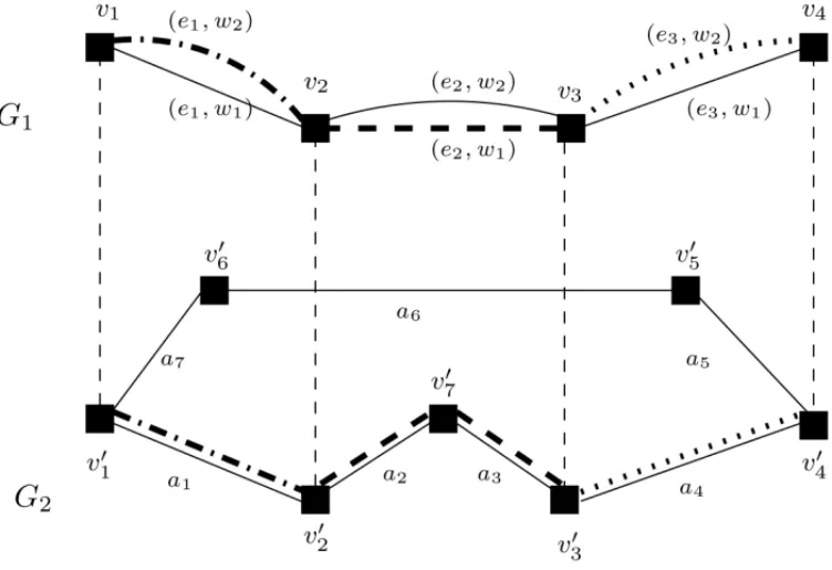
Figure 3 shows an example of solution obtained by solving linear relaxation of the path formu-lation. This instance includes a unique commodity going from nodev1to nodev3. The path in

Figure 3–A solution of the path formulation.

path, namely(e1, w2), is itself assigned the path{a5,a6,a7}inG2, while the pair (e2,w1) is

as-signed the path{a2}inG2. Now suppose that we are looking for new path variables to be added

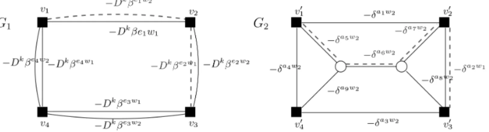
to the current linear programming formulation. Then, Figure 4 shows how dual variables may be distributed on both graphsG1andG2to solve the pricing problems.

Figure 4–GraphsG₁andG₂with dual variables.

Observe that, inG1, the pairs(e1, w2),(e2, w1)that are involved in the routing of our commodity

receive the weights−Dk_βe1w2 _and−Dk_βe2w1_{. The path{(e}

1, w2), (e2, w1)}then has a length

given by−Dkβe1w2_−Dk_βe2w1_{. Note that only dual variables related to pairs(e, w)∈A}

1×Ware

distributed on G1since the fixed term−αk can be considered after shortest path computation.

Similarly, the section (e1, w1) for example is assigned a path in G2 having weights−δa5w2, −δa6w2 _and−δa7w2_{. Again, the weights of arcs inG}

2are only given by dual variables related to

arcs ofA2, while the fixed term given by−γewis added to the length of the shortest path, after

it has been identified.

2.4 Aggregated paths formulation

In this section, we describe an alternative modeling approach for the CMLND-U problem whose purpose is to bypass the utilization of two pricing problems that operate independently. Instead, we attempt to get benefits from the relationship betweenG1andG2to express a

those path variables, and present how the obtained column generation can be integrated within a Branch-and-Price framework.

We will introduce a new notation, sayk, for the set of feasible paths associated with the com-modityk. Now consider the design variables yew_{,e ∈ A}

1, w ∈ W and the commodity path

variablesxk(λ), k ∈ K,λ ∈ k defined in the previous section. For any commodityk ofK, an elementλ ∈ k is actually composed by a pathπ ∈ k AND by a path in Pew for each (e, w)∈π. In order to describe this specific column, we will define a set of coefficients, denoted ϕsuch that for each pair(e, w)∈ A1×W and each arca∈ A2

ϕ_aew(λ)=

1 ifλuses the pair(e, w)inG1and it is assigneda path inG2usinga,

0 otherwise.

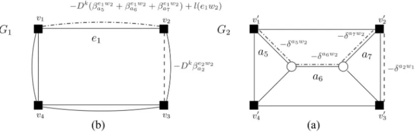
Example 2.1. Figure 5 depicts a path in G1 between nodesv1 andv4, that will be denoted λ. This path is composed by the pairs(e1, w2),(e2, w1)and(e3, w2). Each section ofλis itself

associated with a path in G2. For example,(e2, w1)is assigned the path{a2,a3}. In this example,

coefficientsϕwill take the following values:ϕe1w2

a1 (λ)= 1,ϕ

e2w1

a2 (λ)=ϕ

e2w1

a3 (λ)= 1,ϕ

e3w2

a4 = 1,

whileϕ_aew(λ)= 0 for the remaining entries.

Using this new coefficient, together with the design and commodity path variables, we give the following integer linear programming formulation for the CMLND-U problem:

min

e∈A1

w∈W

c(w)yew

λ∈k

xk(λ)≥1, ∀k∈K, (25)

k∈K

λ∈k

ϕew(λ)Dkxk(λ)≤C yew, ∀e∈ A1, w∈W, (26)

e∈A1

k∈K

λ∈k

ϕ_aew(λ)xk(λ)≤1, ∀a∈ A2, w∈W, (27)

xk(λ)∈ {0,1}, ∀k∈ K, λ∈k, (28) yew ∈ {0,1}, ∀(e, w)∈ A1×W. (29)

In this formulation there is a polynomial number of constraints and design variables, but a huge number of path variables. Observe that all the constraints of the problem are expressed by for-mulation (25)-(29). Indeed, inequalities (25) are the commodity routing constraints. They ensure that a path inG1is associated with each commodity for its routing. Inequalities (26) are the

ca-pacity constraints for every pair(e, w)ofA1×W. Remark that they also appear for eacha∈ A2,

sinceais involved in the definition ofϕ. Inequalities (27) express indirectly the disjunction con-straints for every arca ∈ A2 and every subbandw ∈ W. In fact, each arc a used in a path

associated with some section ofλ(λ∈k, fork∈K) is assigned at most once with subbandw. This formulation will be referred to asaggregated path formulation, and replacing inequalities (28)-(29) by the following

0≤xk(λ)≤1, ∀k∈ K, λ∈k, (30)

0≤yew≤1, ∀(e, w)∈ A1×W. (31)

Yields the linear relaxation of the problem. Notice that, since we projected out subband path variablesz, the solution will be given by a set of subbands to install on the arcs ofG1(given by

the design variables y) as well as a set of paths for commodities routing (given by the variables x). However, it is possible to recover a complete description of the solution for the CMLND-U problem, as coefficientϕ will somehow bring out the path inG2 associated with each pair (e, w)∈ A1×W such thatwis installed one. Similarly to formulation (13)-(19), the number

of commodity path variables here may be exponential. Therefore, using column generation to solve the linear relaxation of (25)-(29) is required. In what follows, we describe the details of the column generation procedure that we propose for the aggregated path formulation.

2.4.1 Column generation

Then we look for the missing paths with negative reduced cost by solving a two-stage pricing problem that we describe here. If such paths are identified, we add them to the RMP and repeat the process until no additional path may be generated.

Let us denote byα,β andδthe dual variables associated with the constraints (25)-(27), respec-tively. The dual variableαis such that for eachk∈ K,αkis inR−,βis such thatβewa ∈R+, for eache∈ A1,w∈W anda ∈ A2. Finally, dual variablesδare such thatδaw ∈ R+. Therefore, the reduced cost related to each commodity path variablexk(λ),k∈ K,λ∈k, is given by the following expression

rck(λ)= −

⎛

⎝αk+

e∈A1

w∈W

a∈A2

ϕ_aew(λ)

Dkβewa+δaw ⎞

⎠.

Hence, we define for each commodityk ∈ K, the pricing problem, as trying to identify a path such thatrck = min{rck(λ) : λ ∈ k}andrck < 0. Note that here, this operation can be performed in two stages. First, dual variablesδare distributed on the arcs ofG2, so that for each (e, w), every arca ∈ A2 receives−δaw. Then, for each (e, w), we compute the shortest path

inG2using the weightsδ. Let us denote by pthis path, andl(e, w)its length. The second step

consists in setting on each pair(e, w)∈ A1×W, a weight given by−Dkβaew+l(e, w), where a ∈ p. This weight is therefore used in order to compute the shortest path inG1between nodes

ok anddk. If the length of the identified path is such thatrck(λ) < 0, then the corresponding commodity path variable should be added to the current linear program.

Note that, even though the generated variable expresses a path in the graphG1, the associated

reduced cost takes into account the dual information impacted on both graphsG1andG2. In this

way, we merge both path variables within a single pricing problem and we still can reconstruct the complete solution thanks to the indicatorϕ.

Example 2.2. Figure 6 shows an example of instance where each set of arcs carries its corre-sponding weight in terms of dual variables. In fact, we can see in Figure 6 (a) the first step of the pricing process, which consists in reporting the weights based on dual variablesδ on each arc of A2.

For example, the shortest path in G2, corresponding to(e1, w2)is {a5,a6,a7}. The length of

this shortest path is a part of the weight assigned to pair(e1, w2), that receives−Dk(βae51w2+

βe1w2

a6 +β

e1w2

a7 )+ l(e1w2), where l(e1w2)= −(δ

a5w2 _+δa6w2 _+δa7w2_{)(see Figure 6 (b)). It}

remains then to compute the shortest path in G1, using weights based on the first step, together

with dual variablesβ.

Notice that all the weights based on the dual variables distributed on the arcs ofG1 andG2

Figure 6–GraphsG1andG2with dual variables (from the aggregated path formulation).

In what follows, we describe how both column generation procedures are embedded within a Branch-and-Bound framework, to get the so-called Branch-and-Price algorithm, and to solve the CMLND-U problem efficiently.

3 BRANCH-AND-PRICE ALGORITHMS

3.1 Overview

Consider given two graphs G1, G2, a set of commodities K and a set of available subbands

W. Also recall that a costc(w) >0 along with a capacity denotedCare associated with each subband ofW. In both path formulations, we consider that this cost increases with the index of the subband. Typically, we letc(w1) ≤ c(w2) ≤ c(w3) ≤ . . . ≤ c(wr), wherer =|W|. This

assumption comes from a practical requirement, that is subbandsi+1 should not be installed before subbandiis installed. In some sense, this assumption is helpful for the model handling, since it also allows to break some symmetries on pairs(e, w)whose total number can be very large in comparison with the few pairs that are actually used in the solution.

To start the optimization, we set up both linear relaxations of (13)-(19) and (25)-(29), restricted to a subset of path variables. The initial subset of path variables is generated using the procedure described in Section 2.3.2 for both formulations. Let us denote by(x,y,z)(respectively(x,y)) the optimal solution of the restricted linear relaxation of path formulation (respectively aggre-gated path formulation). We solve the two pricing problems (respectively the two stage pricing problem), and add the generated path variables to the current LP, if any.

Algorithm 1: Branch-and-Price algorithm for the path formulation

Data :two graphsG1=(V1,A1)andG2=(V2,A2), a set of commoditiesK, a set of

available subbandsW, and a cost vectorc∈ IRW.

Output :optimal solution of CMLND-U problem, or best feasible upper bound.

1: LP←LPinit ial;

2: solve the linear program LP;

let(x,y,z)be the optimal solution of LP;

3: Consider the dual variables and solve the two pricing problems; 4:Iffor all(e, w)∈ A1×W,p∈ Pew,rcew >0then

5: Iffor allk∈ K,π ∈k,rck >0then

6: go to 10;

7: else

8: Add the variables induced byrcew andrcew with negative reduced cost;

9: go to 2

10:If(x,y,z)is integerthen

11: (x,y,z)is optimal for CMLND-U. Stop; 12:else

13: Create two sub-problems by branching on design variables first; 14:forallopen sub-problemdo

15: go to 2;

16:returnthe best optimal solution for all sub-problems.

3.2 Branching

Let(P)denote the linear program at a given node of the Branch-and-Bound tree. Suppose that the optimal solution of linear relaxation of(P_{)is fractional. Let(x,y,z)be this fractional solution.}

The branching phase, consists in choosing a fractional variable sayx1among those in(x,y,z), and create two sub-problems(P_1)and(P_{2)by adding either constraintx}1_{≤ ⌊x}1_⌋orx1_{≥ ⌈x}1_⌉

to(P_{). In our problem, it is to fixx}1_{either to 0 or 1.}

In our case, we have observed that branching first on design variables was very effective in prac-tice, and only few path variables remain fractional after that, for both formulations. This can be explained by the strong relationship between those families of variables in both formulations. Thus, we have used the following strategy. First we perform branching on fractional design vari-ablesyby choosing the variable with fraction close to 0.5 and high absolute objective function coefficient. Fixing design variables helps to get few remaining path variables that still fractional. If all the design variables are integer, then we perform branching on path variables by setting their value either to 0 or 1.

Based on these features, we have implemented our Branch-and-Price algorithms for the CMLND-U problem by solving both the path and aggregated path formulations. We have tested our approaches on a set of random and SNDlib based instances. The obtained results are shown and reviewed in the coming section.

4 COMPUTATION EXPERIMENTS

4.1 Implementation’s feature

We have implemented the Branch-and-Price algorithms described in the previous section in C++ using ABACUS 3.2 [1] to handle the Branch-and-Price tree, and CPLEX 12.5 [2] as LP solver. Our approach was tested on a processor Intel Core i5-3210M CPU 2.50 GHz×4 with 3.7 Gb RAM, running under ubuntu 12.10 platform. We fixed the maximum CPU time to 3 hours.

Both algorithms were tested on random and realistic instances. The realistic instances are ob-tained from SNDlib data for instancesdfn bwin,dfn gwin,newyorkandfrance. The entries of the different tables presented in the sequel are the following:

V2 : number of nodes inG2,

A2 : number of arcs,

K : number of commodities,

Gap : the relative distance between the best upper bound (optimal solution if the problem has been solved to optimality) and the lower bound obtained provided by the compact formulation,

columns : number of generated path variables,

nodes : number of nodes in the Branch-and-Cut tree, TT : total CPU time in h:m:s

TTpricing : CPU time spent in pricing out path variables (in %).

4.2 Managing infeasibility

each(e, w)∈ A1×W. Variablesτ are involved in inequalities (13) (path formulation) and (25)

(aggregated path formulation), whileθappears in inequality (15) in path formulation.

Notice that we do not use such variables in inequalities (14), (16), (26), and (27), since fixing variables to 0 does not affect feasibility of those constraints. We associate with all the artificial variables a large cost in the objective function, so as to avoid using them unnecessarily in the solution. However, these variables ensure that a feasible solution, even costly, can always be identified.

4.3 Computational results

Our first series of experiments involve random instances, whose topologies as well as the com-modities were randomly generated. We have considered connected graphs with 6 to 14 nodes, and at most 18 commodities per instance. Tables 1 and 2 report the results given by the column generation and the Branch-and-Price approaches on solving both path and aggregated path for-mulations, for random instances. The reported results concern 35 instances with a number of nodes in the physical layer (graphG2) varying from 6 to 14 nodes, and a number of arcs varying

from 16 to 40. We have considered up to 18 commodities for each kind of graph, and the number of available subbands is|W|= 4 except for the 14 nodes instances where|W|= 5.

Table 1 shows in particular the results obtained by both column generation procedures for linear relaxation of formulations (13)-(19) and (25)-(29). The two last columns contain results provided by the compact formulation, namely the gap and CPU time computation. Note that the compact formulation is solved by Branch-and-Bound procedure. It appears from this table that the gap provided by the path formulation is equivalent to the one of the compact formulation. Indeed, this is predicted by theory, since we are replacing flow constraints in the compact formulation by their equivalent representation in terms of paths. We also remark that for most of the instances, the gap provided by the path formulation is better than the one of the aggregated path formulation. In fact, except for instances with|V2|= 6,|K|= 8, 10 and 11, and|V2|= 14,|K|= 8, the gap value for the path formulation is smaller than the one of the aggregated path formulation.

We can see that our column generation procedures do not behave the same way for both path formulations. Indeed, although the number of generated variables in the first procedure is not so important (less than 100 path variables, except for the last instance), it is significantly higher for the second procedure. This can be due to the fact that the aggregated approach might somehow induce a loss of information provided by the bi-layer structure of the problem, and the interaction between the path variables in both graphsG1andG2.

Table 1–Comparing linear relaxations.

Compact Path Aggregated path

formulation formulation formulation

|V2| |A2| |W| |K| Gap (%) Columns Gap (%) Columns

6 16 4 2 25.00 8 25.00 39

6 16 4 4 47.50 16 47.50 73

6 16 4 6 45.00 24 53.33 86

6 16 4 8 41.43 32 37.14 211

6 16 4 10 47.14 49 41.43 281

6 16 4 12 48.75 57 43.75 165

8 24 4 2 0.00 8 0.00 51

8 24 4 4 25.00 16 25.00 95

8 24 4 6 33.33 24 33.33 140

8 24 4 8 6.25 36 6.25 147

8 24 4 10 15.50 40 28.00 223

8 24 4 12 12.92 48 26.67 211

8 24 4 14 21.92 56 25.38 311

8 24 4 16 32.31 68 33.08 377

8 24 4 18 35.63 76 36.25 383

10 36 4 2 0.00 8 0.00 64

10 36 4 4 50.00 16 50.00 139

10 36 4 6 3.33 24 3.33 524

10 36 4 8 44.44 38 55.55 381

10 36 4 10 57.31 46 59.23 433

10 36 4 12 56.07 54 57.86 533

12 46 4 2 0.00 8 0.00 80

12 46 4 4 33.33 16 33.33 165

12 46 4 6 46.67 24 46.67 433

12 46 4 8 47.14 33 47.14 598

12 46 4 10 33.13 41 37.50 668

12 46 4 12 20.63 49 25.00 1047

14 40 5 2 0.00 11 25.00 218

14 40 5 4 0.00 21 12.50 768

14 40 5 6 14.29 31 14.29 799

14 40 5 8 44.40 46 41.11 693

14 40 5 10 37.51 50 39.23 1079

14 40 5 12 10.63 61 11.92 836

14 40 5 14 34.47 71 35.00 943

14 40 5 16 12.47 130 20.59 1103

A M A L B E NHA M ICHE , A . R IDHA M A HJ O U B , NA NCY P E R R O T a n d E D U A RDO UCHO A

Compact formulation Path formulation Aggregated path formulation

|V2| |A2| |W| |K| TT columns nodes TT TTpricing (%) columns nodes TT TTpricing (%)

6 16 4 2 00:05:32 8 3 00:00:01 0 98 3 00:00:00 72

6 16 4 4 00:07:53 24 107 00:00:02 17 467 31 00:00:02 74

6 16 4 6 00:10:49 36 219 00:00:23 19 119 5 00:00:01 81

6 16 4 8 00:49:32 39 403 00:00:04 18 234 11 00:00:04 88

6 16 4 10 01:00:23 399 3893 00:00:49 21 457 11 00:00:03 93

6 16 4 12 01:45:03 6249 24819 00:03:45 19 357 11 00:00:02 92

8 24 4 2 00:08:56 8 1 00:00:01 0 51 1 00:00:01 54

8 24 4 4 00:21:51 16 15 00:00:01 9 97 15 00:00:01 63

8 24 4 6 00:29:23 24 65 00:00:03 17 143 65 00:00:03 87

8 24 4 8 01:02:14 32 65 00:00:03 22 415 3 00:00:02 92

8 24 4 10 01:12:09 40 1189 00:00:26 18 378 5 00:00:01 88

8 24 4 12 01:02:14 48 2585 00:00:59 19 670 5 00:00:01 89

8 24 4 14 02:31:46 56 2048 00:08:31 18 688 10 00:00:03 86

8 24 4 16 02:49:01 74 3280 00:16:44 18 598 7 00:00:01 91

8 24 4 18 02:52:21 82 3580 00:17:00 19 720 15 00:00:23 89

10 36 4 2 00:10:37 8 1 00:00:00 27 64 1 00:00:00 82

10 36 4 4 00:18:22 16 73 00:00:05 15 150 9 00:00:04 88

10 36 4 6 00:32:51 62 127 00:00:06 18 645 11 00:00:12 79

10 36 4 8 01:44:02 205 859 00:01:18 18 436 17 00:00:20 82

10 36 4 10 02:05:39 481 3559 00:03:06 20 543 23 00:00:57 86

10 36 4 12 02:55:01 1060 18527 00:28:46 19 712 159 00:01:39 88

12 46 4 2 01:15:22 8 1 00:00:00 20 80 1 00:00:01 87

12 46 4 4 01:35:22 16 73 00:00:11 14 165 1 00:00:01 86

12 46 4 6 02:09:59 77 127 00:00:12 17 650 17 00:00:04 87

12 46 4 8 02:23:51 52 801 00:01:17 17 670 15 00:00:03 88

12 46 4 10 02:45:33 40 1695 00:02:44 18 769 7 00:00:07 91

12 46 4 12 03:00:00 260 509 00:01:30 24 2610 117 00:00:02 92

14 40 5 2 01:49:32 11 1 00:00:00 17 218 1 00:00:00 79

14 40 5 4 02:33:01 26 1 00:00:00 31 932 179 00:00:58 85

14 40 5 6 03:00:00 36 17 00:00:08 13 1079 237 00:01:01 92

14 40 5 8 03:00:00 112 491 00:03:25 13 1011 559 00:01:59 89

14 40 5 10 03:00:00 502 2771 00:18:49 15 2392 3591 00:20:53 95

14 40 5 12 03:00:00 786 2771 00:19:12 18 1221 2375 00:16:41 93

that, except for some instances, the number of variables generated within the second Branch-and-Price algorithm is still higher than the one in the first Branch-Branch-and-Price. Also we can remark that most of the added variables are generated at the root node of the Branch-and-Price tree for both algorithms. It should be pointed out that the number of nodes in the first Branch-and-Price tree is more important than in the second Branch-and-Price tree. In other words, we can observe that in the second algorithm, most of the columns are generated in the upper level nodes of the tree. By contrast, there is a sparsity in the first Branch-and-Price tree where fewer columns are generated along a large-size tree.

Our second series of experiments concern realistic instances based on data from SNDlib for networksdfn bwin,dfn gwin,newyorkandfrance. Those instances have graphs with 10 to 25 nodes, while the number of commodities varies between 4 and 30 for dfn gwin and newyork (we have considered up to 18 commodities for dfn bwin and 16 commodities for france). The results of the Branch-and-Price algorithm based on the double column generation are summarized in Table 3. Table 4 shows the results provided by the Branch-and-Price algorithm using the two-stage column generation.

It appears from Table 3 that all the considered instances have been solved to optimality using the Branch-and-Price approach, within the fixed time limit. In fact, 30 instances have been solved to optimality in less than 10 minutes. Moreover, note that 11 among the 40 tested instances were solved to optimality at the root node. This can show that our data-preprocessing performs well on realistic instances. Due to the size and structure of some instances, we can observe that the CPU time spent by the algorithm in pricing operations increases compared to its average value for random instances (see Table 1). However, the number of generated columns in the whole tree is not so important regarding to the size of the instances. This is allowed by our procedure to generate initial paths, that helps to identify a first set of interesting variables and thus to form a good initial basis. For the remaining instances, the number of generated path increases with the size of the instance, except for some instances where our algorithm may have atypical behavior. Basically, more path variables are generated for instance newyork with|K|= 25, than for instance newyork with|K|= 30. We can explain such a result by the fact that the routing of some commodities may be challenged by the size (traffic amount) of other commodities. Indeed, the more commodities will induce “conflicts” due to their size and the subband capacity, the more an instance will be difficult to solve. Indeed, in this case many arcs might be saturated, thus requiring further path to be explored in order to identify feasible (and good) solutions.

Table 4 shows the results of Branch-and-Price algorithm for the aggregated path formulation. We can see from this table that this algorithm, similarly to the previous one, allowed to solve to optimality all the tested instances within the CPU time limit. Observe that the gap values are quite comparable to those presented in Table 3. Also remark that, similarly to column generation procedures, both Branch-and-Price algorithms do not work in the same way.

Table 3–Branch-and-Price results for SNDlib-based instances – Path formulation.

Instance |V2| |A2| |W| |K| Gap (%) columns nodes TT TTpricing (%)

dfn bwin 10 90 4 2 25.00 8 3 0:00:00.28 28.5714%

dfn bwin 10 90 4 4 12.50 16 3 0:00:00.28 28.5714%

dfn bwin 10 90 4 6 8.33 41 3 0:00:00.37 45.9459%

dfn bwin 10 90 4 8 43.75 166 397 0:00:26.60 31.8797%

dfn bwin 10 90 4 10 40.00 247 859 0:00:44.09 32.4563%

dfn bwin 10 90 4 12 29.17 49 381 0:00:19.66 29.5015%

dfn bwin 10 90 4 14 27.59 81 2419 0:02:08.20 30.4992 %

dfn bwin 10 90 4 16 27.27 510 4265 0:04:00.16 32.82 %

dfn bwin 10 90 4 18 26.32 219 5913 0:05:42.10 31.48 %

dfn gwin 11 94 4 2 0.00 10 1 0:00:00.44 36.36 %

dfn gwin 11 94 4 4 0.00 20 1 0:00:00.44 34.0909%

dfn gwin 11 94 4 6 0.00 36 1 0:00:00.40 52.5%

dfn gwin 11 94 4 8 0.00 53 1 0:00:00.5 66.0714%

dfn gwin 11 94 4 10 0.00 60 1 0:00:00.52 59.6154%

dfn gwin 11 94 4 12 0.00 78 1 0:00:00.39 58.9744%

dfn gwin 11 94 4 14 0.00 89 1 0:00:00.42 59.5238%

dfn gwin 11 94 4 16 5.88 117 7 0:00:02.03 43.34 %

dfn gwin 11 94 4 18 19.44 133 587 0:01:41.22 28.37 %

dfn gwin 11 94 4 20 25.00 2499 2755 0:10:50.70 34.05 %

dfn gwin 11 94 4 25 21.28 1620 2931 0:10:47.54 33.10 %

dfn gwin 11 94 4 30 20.41 830 2931 0:10:32.60 31.08 %

newyork 16 92 5 2 0.00 10 1 0:00:00:10 28.5714%

newyork 16 92 5 4 0.00 20 1 0:00:00.72 33.33 %

newyork 16 92 5 6 0.00 30 1 0:00:00.77 36.36 %

newyork 16 92 5 8 37.50 567 807 0:08:09.32 26.46 %

newyork 16 92 5 10 40.00 172 2905 0:16:03.30 27.62 %

newyork 16 92 5 12 41.67 1358 6331 0:49:34.92 26.95 %

newyork 16 92 5 14 0.00 104 1 0:00:01.30 58.4615%

newyork 16 92 5 16 6.25 114 35 0:00:13.78 31.35 %

newyork 16 92 5 18 16.67 90 221 0:02:10.97 29.31 %

newyork 16 92 5 20 20.00 100 659 0:07:01.98 28.73 %

newyork 16 92 5 25 20.00 148 4165 0:29:09.84 31.84 %

newyork 16 92 5 30 20.00 100 659 0:06:44.59 29.06 %

france 25 90 5 2 50.00 10 23 0:00:35.99 11.86 %

france 25 90 5 4 37.50 20 91 0:02:25.19 13.75 %

france 25 90 5 6 41.67 30 147 0:06:33.75 15.57 %

france 25 90 5 8 37.50 40 511 0:25:54.95 17.28 %

france 25 90 5 10 40.00 50 2611 1:18:20.44 19.385%

france 25 90 5 12 33.33 60 1987 3:00:00 23.526%

france 25 90 5 14 21.43 70 2245 3:00:00 25.03 %

france 25 90 5 16 26.03 2639 16581 3:00:00 45.23 %

Table 4–Branch-and-Price results for SNDlib-based instances – Aggregated path formulation.

Instance |V2| |A2| |W| |K| Gap (%) columns nodes TT TTpricing (%)

dfn bwin 10 90 4 2 0.00 129 1 0:00:03.04 87.75%

dfn bwin 10 90 4 4 12.50 340 3 0:00:04.55 92.70%

dfn bwin 10 90 4 6 8.33 546 15 0:00:12.00 92.83%

dfn bwin 10 90 4 8 43.75 588 23 0:00:57.00 89.17 %

dfn bwin 10 90 4 10 40.00 724 23 0:01:33.00 92.52 %

dfn bwin 10 90 4 12 29.17 873 35 0:01:44.00 93.46 %

dfn bwin 10 90 4 14 27.59 1023 129 0:03:56.00 92.08 %

dfn bwin 10 90 4 16 27.27 1165 253 0:16:32.00 90.38 %

dfn bwin 10 90 4 18 26.32 876 311 0:20:31.00 94.17 %

dfn gwin 11 94 4 2 0.00 241 1 0:00:05.47 94.14%

dfn gwin 11 94 4 4 0.00 537 1 0:00:14.53 98.21%

dfn gwin 11 94 4 6 0.00 448 1 0:00:09.38 96.80%

dfn gwin 11 94 4 8 0.00 658 1 0:00:10.77 97.02%

dfn gwin 11 94 4 10 10.23 785 3 0:00:19.07 95.96%

dfn gwin 11 94 4 12 13.00 688 7 0:00:57.00 86.83%

dfn gwin 11 94 4 14 8.73 843 7 0:01:39.00 87.92%

dfn gwin 11 94 4 16 32.98 926 17 0:03:28.00 93.96%

dfn gwin 11 94 4 18 5.88 1023 51 0:08:05.00 92.22%

dfn gwin 11 94 4 20 19.44 876 101 0:10:55.00 88.9%

dfn gwin 11 94 4 25 25.00 947 127 0:14:48.00 91.9%

dfn gwin 11 94 4 30 21.28 1034 205 0:28:34.00 94.38%

newyork 16 92 5 2 20.41 526 3 0:00:37.80 95.74 %

newyork 16 92 5 4 12.50 830 7 0:00:50.26 95.80 %

newyork 16 92 5 6 33.2 2188 19 0:02:29.30 94.86 %

newyork 16 92 5 8 25.00 1634 239 0:03:28.00 88.9%

newyork 16 92 5 10 37.50 1435 431 0:07:31.00 89.32 %

newyork 16 92 5 12 40.00 1289 511 0:21:58.00 91.43 %

newyork 16 92 5 14 41.67 2076 873 0:00:12.00 88.74 %

newyork 16 92 5 16 12.50 2198 1021 0:16:53.00 91.28 %

newyork 16 92 5 18 6.25 4389 3287 0:20:42.00 90.33 %

newyork 16 92 5 20 16.67 3741 2719 0:26:18.00 91.28 %

newyork 16 92 5 25 20.00 3827 2501 1:08:37.00 92.33 %

newyork 16 92 5 30 20.00 4659 3283 1:40:53.00 88.84 %

france 25 90 5 2 20.00 51 1 0:00:03.00 90.33 %

france 25 90 5 4 50.00 88 3 0:01:48.00 94.37 %

france 25 90 5 6 37.50 103 7 0:01:44.00 95.12 %

france 25 90 5 8 41.67 114 7 0:00:53.00 94.22 %

france 25 90 5 10 37.50 2378 537 0:43:37.95 88.54 %

france 25 90 5 12 40.00 3439 721 1:40:20.44 89.17 %

france 25 90 5 14 33.33 4392 1077 2:37:48.76 90.27 %

france 25 90 5 16 21.43 5283 1259 2:10:30.09 95.39 %

translate an explicit definition of path variables associated with both physical and virtual layer, to an embedded definition of variables. In other words, the aggregated path formulation performs better, since we handle a unique family of “double” path variables (defined inG1but implicitly

related to a path inG2), instead of two families, which is somehow easier.

5 CONCLUDING REMARKS

In this paper we have introduced a compact formulation for the CMLND-U problem. Based on this formulation, we have derived two different path formulations for the problem. The first one considers an explicit decomposition approach, and induces a column generation procedure requiring two pricing sub-problems. The second model, namely aggregated path formulation, attempts to give an implicit decomposition of the problem, where the virtual layer includes in-formations of the physical layer. This is allowed by a new family of path variables that have a specific structure and can be priced out with a unique subproblem. We have devised a Branch-and-Price algorithm to solve each of the formulations and compared the obtained results to show empirically that they are more efficient than a Branch-and-Bound for the compact formulation. Finally, we have presented some experiments to show the effectiveness of our approach and to compare both algorithms.

We could see that both Branch-and-Price algorithms perform generally well on the tested in-stances but can be still enhanced. Indeed, Several interesting perspectives can be considered to boost their performances. For instance, we could consider more sophisticated branching strat-egy to handle the size of Branch-and-Price tree concerning the first path formulation. Besides, a deeper investigation of the pricing problem for the aggregated formulations should enable to better control the column generation procedure. Finally, a good primal heuristic should allow to prune much more efficiently the nodes of the tree whose exploration is not relevant.

ACKNOWLEDGMENTS

Authors are very grateful to the anonymous referees for their constructive comments on a previ-ous version of the paper.

REFERENCES

[1] http://www.informatik.uni-koeln.de/abacus/.

[2] http://www-01.ibm.com/software/integration/optimization/ cplex-optimizer/.

[3] AHUJARK, MAGNANTITL & ORLINJB. 1993.Network flows: theory, algorithms, and applica-tions. Prentice-Hall, Inc.

[4] AVELLAP, MATTIAS & SASSANOA. 2007. Metric inequalities and the network loading problem. Discrete Optimization,4(1): 103–114.

[6] BELOTTIP, CAPONEA, CARELLOG & MALUCELLIF. 2008. Multi-layer mpls network design: The impact of statistical multiplexing.Computer Networks,52(6): 1291–1307.

[7] BENHAMICHEA, MAHJOUBAR, PERROTN & UCHOAE. Capacitated multi-layer network de-sign with unsplittable demands: Polyhedra and branch-and-cut (technical report).https://www. lamsade.dauphine.fr/sites/default/IMG/pdf/cahier\_383.pdf, 2017.

[8] BORNES, GOURDINE, LIAUB & MAHJOUBAR. 2006. Design of survivable ip-over-optical net-works.Annals of Operations Research,146(1): 41–73.

[9] DAHLG, MARTINA & STOERM. 1999. Routing through virtual paths in layered telecommunication networks.Operations Research,47(5): 693–702.

[10] DIJKSTRAEW. 1959. A note on two problems in connexion with graphs.Numerische Mathematik, 1(1): 269–271, December.

[11] FEILLETD. 2010. A tutorial on column generation and branch-and-price for vehicle routing prob-lems.4OR,8(4): 407–424.

[12] FORTZB & POSSM. 2009. An improved benders decomposition applied to a multi-layer network design problem.Operations Research Letters,37(5): 359–364.

[13] HOLLERH & VOSSS. 2006. A heuristic approach for combined equipment-planning and routing in multi-layer sdh/wdm networks.European Journal of Operational Research,171(3): 787–796. [14] HUJQ & LEIDAB. 2004. Traffic grooming, routing, and wavelength assignment in optical wdm

mesh networks. In:Proceedings of the IEEE INFOCOM 2004, pages 495–501.

[15] KNIPPELA & LARDEUXB. 2007. The multi-layered network design problem.European Journal of Operational Research,183(1): 87–99.

[16] MATTIAS. 2013. A polyhedral study of the capacity formulation of the multilayer network design problem.Networks.

[17] ORLOWSKIS, KOSTERAMCA, RAACKC & WESSALY¨ R. 2007. Two-layer network design by branch-and-cut featuring mip-based heuristics. In: Proceedings of the INOC 2007 also ZIB Report ZR-06-47, Spa, Belgium.

[18] ORLOWSKIS, RAACKC, KOSTERAMCA, BAIERG, ENGELT & BELOTTIP. 2010. Branch-and-cut techniques for solving realistic two-layer network design problems. In:Graphs and Algorithms in Communication Networks, pages 95–118. Springer Berlin Heidelberg.

[19] RAGHAVANS & STANOJEVI´CD. 2011. Branch and price for wdm optical networks with no bifur-cation of flow.INFORMS J. on Computing,23(1): 56–74.

[20] RYANDM & FOSTERBA. 1981. An integer programming approach to scheduling. In: Computer Scheduling of Public Transport: Urban Passenger Vehicle and Crew Scheduling, pages 269–280.

[21] VANDERBECKF. 1994.Decomposition and column generation for integer programming. PhD thesis, Universit´e Catholique de Louvain, Belgium.

[22] VANDERBECKF. 2000. On dantzig-wolfe decomposition in integer programming and ways to per-form branching in a branch-and-price algorithm.Operations Research,48(1): 111–128.

[23] VANDERBECKF. 2005. Implementing mixed integer column generation. In Guy Desaulniers, Jacques Desrosiers, and MariusM. Solomon, editors,Column Generation, pages 331–358. Springer US.

[24] ZHUK & MUKHERJEEB. 2002. Traffic grooming in an optical wdm mesh network.IEEE Journal