Are all lenders equal? a comparison between peer-to-peer lending and traditional banks concerning small business loans

(1)

FUNDAÇÃO GETULIO VARGAS

ESCOLA BRASILEIRA DE ADMINISTRAÇÃO PÚBLICA E DE EMPRESAS MESTRADO EM ADMINISTRAÇÃO

ARE ALL LENDERS EQUAL? A COMPARISON BETWEEN

PEER-TO-PEER LENDING AND TRADITIONAL BANKS

CONCERNING SMALL BUSINESS LOANS

DISSERTAÇÃO APRESENTADA À ESCOLA BRASILEIRA DE ADMINISTRAÇÃO

PÚBLICA E DE EMPRESAS PARA OBTENÇÃO DO TÍTULO DE MESTRE

SHENGJIE ZHANG

Rio de Janeiro - 2019

(2)

Dados Internacionais de Catalogação na Publicação (CIP) Ficha catalográfica elaborada pelo Sistema de Bibliotecas/FGV

Zhang, Shengjie

Are all lenders equal? : comparison between peer-to-peer lending and traditional banks concerning small business loans / Shengjie Zhang. – 2019.

37 f.

Dissertação (mestrado) - Escola Brasileira de Administração Pública e de Empresas, Centro de Formação Acadêmica e Pesquisa.

Orientador: Lars Norden. Inclui bibliografia.

1. Pequenas e médias empresas – Empréstimos. 2. Empréstimo bancário. 3. Crédito bancário. I. Norden, Lars. II. Escola Brasileira de Administração Pública e de Empresas. Centro de Formação Acadêmica e Pesquisa. III. Título. CDD – 332.1753

(3)

(4)

1

Are All Lenders Equal?

A Comparison between Peer-to-Peer Lending and

Traditional Banks Concerning Small Business Loans

Shengjie Zhang1

EBAPE, Getúlio Vargas Foundation

Academic Advisor:

Lars Norden2

EBAPE, Getúlio Vargas Foundation

Abstract

Research on geographical expansion of peer-to-peer lending platforms has different conclusions concerning whether peer-to-peer lending platforms and traditional banks are substitutes or complements. This study aims at exploring factors that affect the expansion of peer-to-peer lending platform with respect to small business loans and finding out whether peer-to-peer lending platforms are substitutes or complements to banks concerned with small business loans. LendingClub is taken as the representative of peer-to-peer lending platforms as it is the largest one in the United States. I draw heat maps based on the normalized share of LendingClub to the total small business loan market. Multiple regression and quantile regression are used to fit the regression models. The study shows that LendingClub tend to have higher market share in areas where there are more small business credit demands. Secondly, LendingClub has more market share in areas where the male ratio is higher, and local economies are not well developed, as the high unemployment rate and low income can significantly increase the market share of LendingClub. Thirdly, bank and LendingClub may be substitutes to each other in terms of small business loans as the change of bank branch is insignificantly negatively related to the market share of LendingClub in the main analysis and has a significantly negative influence on the market share of LendingClub in state-level robustness test.

Keywords: Geographical expansion, heat map, P2P, small business loan

1_{Msc student in Brazilian School of Public and Business Administration (EBAPE), Getúlio Vargas Foundation, Rua}

Jornalista Orlando Dantas 30, 22231-010 Rio de Janeiro, Brazil, E-mail:shengjie.zhang@fgv.edu.br

2_{Professor in Brazilian School of Public and Business Administration (EBAPE), Getúlio Vargas Foundation, Rua}

Jornalista Orlando Dantas 30, 22231-010 Rio de Janeiro, Brazil, E-mail:lars.norden@fgv.edu.br

I am grateful for the guidance of Professor Lars Norden and the suggestions and help from Professor Fabio Caldieraro and Professor Jéfferson Augusto Colombo.

(7)

4

1. Introduction

Small businesses are firms with fewer than 500 employees according to the U.S. Small Business Administration (SBA). In that sense, more than 99 percent of the firms in the United States are

small businesses, and about 50 percent are firms with less than 5 employees3_{. Therefore, small}

businesses’ credit source becomes an important issue, because credit is critical for these businesses evolving into bigger firms (Brown et al., 1990; De la Torre, 2008).

Nevertheless, small business has difficulty in gaining credit capitals. Studies show that when firms are young or small, the problem of adverse selection and moral hazard can be more serious (Berger and Udell, 1995; Petersen and Rajan, 1994). Consequently, the most common capital source for small businesses is the owner’s personal loan. According to the Annual Survey of Entrepreneurs (Foster and Norman, 2016), in 2014, about 55 percent of small business entrepreneurs gain their start-up capitals through loans from owners, followed by financing from banks, loans from family and friends and other resources. As for personal loans, 73.2 percent of the small businesses owners regard commercial bank as their primary choice, as the 2013 Survey of Consumer Finances (SCF) indicated (Bricker et al., 2012).

Even though, with the popularity of the online community and the appearance of FinTech, peer-to-peer lending (P2P) becomes an increasingly important financial resource for personal loans. The idea of P2P lending is actually loan-based crowdfunding (Kavuri and Milne, 2019). Until now, the most popular online P2P lending platforms are Prosper and LendingClub, which were launched in 2007 in the US. For the past ten years, the volume of P2P lending has been growing rapidly. Until 2015, the volume of LendingClub is over 8 billions of dollars, more than half of that of Prosper (Havrylchyk et al., 2018).

Current literature about P2P lending focuses on the difference of the loan performance of P2P platform and banks (Mach et al., 2014) and the soft information that can affect the performance and loan success rate of P2P platform (Freedman and Jin, 2017; Lin, 2009; Xu and Chau, 2018a). Few studies focus on the spatial expansion of P2P lending. Jagtiani and Lemieux use LendingClub data concerned with consumer loans from 2014 to 2016 and explore the factors that may cause the

(8)

5

spatial difference of LendingClub and banks (Jagtiani and Lemieux, 2018). Havrylchyk et al include both LendingClub and Prosper data in all fields from 2006 to 2013 and study what drive the expansion of the peer-to-peer lending (Havrylchyk et al., 2018).

In this paper, I explore the spatial distribution of LendingClub small business lending, compare it with commercial bank small business lending, and find out factors that cause the regional difference. In addition, I also want to answer the question “Are P2P lending and bank substitutes or complements”. Previous literature does not reach a consistent conclusion to this question. Some studies find that P2P lending and bank lending are complements (Damar, 2009; Tang, 2019). Tang et al find that the credit expansion resulting from P2P lending likely occurs only among borrowers who already have access to bank credit (Tang, 2019), while Darmar et al find that payday lenders enter areas that are already served by banks (Damar, 2009). Other studies, for example, Havrylchyk et al find that borrowers are more likely to borrow from P2P lending platforms when the region they live have lower leverage ratios (Havrylchyk et al., 2018).

The rest of the paper is organized as follows. Section 2 presents the literature review and hypotheses. Section 3 describes the sources of the data that I use and how I transform them according to our research purpose. In section 4, I draw the choropleth maps of the share of LendingClub and list out the top 20 counties that have a high share of LendingClub. Section 5 illustrates the empirical results including description analysis, multiple regression, and quantile regression. Section 6 is the robustness tests. Section 7 concludes and provides suggestions for future study.

2. The Literature and Hypotheses

I explore previous literature to see what are the main factors that can have an influence on the penetration of P2P lending. Buchak et al focus on the expansion of shadow bank. They use the data of both shadow banks and traditional banks from 2007 to 2015 and find that lower income borrowers, racial minorities, male borrowers are more likely to be shadow bank borrowers (Buchak et al., 2018). Enrichetta studies the effect of beauty and personal characteristics in credit markets, using Prosper’ data from March to June 2007 and finds that beautiful borrowers and women are

(9)

6

more likely to get loans, while Black and Asian borrowers are less likely to get loans (Enrichetta, 2019).

In addition to the above studies, there are some articles that study the regional difference of the P2P lending market. Havrylchyk et al rely on loan book data from LendingClub and Prosper from 2006 to 2013, and include financial crisis variables, bank branch density as proxy for entry barriers, socio-demographic variable to represent learning costs, patents per capita as proxy for openness to innovation and other variables such as income per capita, unemployment rates, poverty rate and race (Havrylchyk et al., 2018). They find that P2P lending platforms are partly substituted for banks in counties that are more affected by the financial crisis. High market concentration and high branch density deter the expansion of P2P, while education, population density, and young people ratio decrease learning costs and promote the expansion of P2P.

Jagtiani and Lemieux study the factors that may affect the expansion of LendingClub consumer loans from 2013 to 2016 (Jagtiani and Lemieux, 2018). They include unemployment rate, home price index, income per capita and population density as proxies for the economic environment; bank branches and percent change in bank branch as proxies for deposit activities and branching data; and HHI as a proxy for credit card market concentration. They find that the number of branches and the local economy is negatively related to the volume of LendingClub, and market concentration is positively related to the volume of LendingClub.

Tang focuses on the question of whether P2P lending platform serves as substitutes or complements for banks (Tang, 2019). He fits the factors into the regression discontinuity model with the LendingClub data from 2009 to 2012 and includes HHI as a proxy for market concentration, population, personal income, deposits, and unemployment as control variables. He finds that P2P lending and bank lending are substitutes with respect to infra-marginal bank borrowers and are complements in terms of small loans.

From the above literature review, I include three categories of factors that may affect the expansion of P2P lending, geographical environment, macroeconomic environment, and local activities, as the following illustrates.

(10)

7

2.1 Geographical Environment

2.1.1 Race

Race is the most important geographical factor that determines whether the person would prefer online lending from p2p platforms or traditional lending from banks. Blanchflower et al use the data from the 1993 and 1998 National Surveys of Small Business Finances and find that black-owned small businesses are twice less likely to gain credit loans (Blanchflower et al., 2006). Recent research also shows that black borrowers are less likely to get loans from banks in areas where racial prejudice is high (Enrichetta, 2019). Therefore, I hypothesize that black people are more likely to borrow money online and therefore

H1: In areas where white ratio is higher, the share of Lending Club will be lower.

2.1.2 Gender

Gender is another important geographical factor accounting for the utilization of the online peer-to-peer lending platform. Firstly, men are considered to use the Internet more than women even though the gap is narrowed through all these years (Dholakia, 2006). This may cause men to have more tendency to use the online peer-to-peer lending platform to get loans rather than go to the bank and talk with the officer. Secondly, men are usually more interested in financial websites than women when using the Internet (Wasserman and Richmond-Abbott, 2005). This may also lead them to get to know the concept of peer-to-peer lending and thus makes them have more tendency to seek loans through the Internet. Thirdly, however, women are usually discriminated when seeking capitals(Bellucci et al., 2010; Fay and Williams, 1993), thus, they may have less tendency to seek capitals through traditional banks and be more likely to seek capitals through the peer-to-peer lending platform online. Nevertheless, recently, some research found the completely different phenomenon, that female entrepreneurs are less likely to be credit constrained than male (Wellalage and Locke, 2017). Previous studies show that female are less likely to borrow money online (Buchak et al., 2018). Considering the above facts, I hypothesize that,

H2a: In areas where male ratio is higher, the share of Lending Club will be higher. H2b: In areas where male ratio is higher, the share of Lending Club will be lower.

(11)

8

2.2 Macroeconomic Environment

In addition to geographical factors, macroeconomic environment in a certain region would also affect borrowers’ choice of loan resources. Increase in money supply, exchange rate, unemployment rate, inflation rate, and interest rate can increase banks’ credit risks (Yurdakul, 2014). Buchak et al find that lower income borrowers are more likely to be shadow bank borrowers (Buchak et al., 2018). Jagtiani and Lemieux find that unemployment rate is negatively related to the share of Lending Club, while income per capita, home price index and year dummy is positively related to borrowing money from Lending Club (Jagtiani and Lemieux, 2018). Therefore, I hypothesize,

H3: Unemployment rate is positively related to the share of Lending Club. H4: Income is negatively associated with the share of Lending Club. H5: Year is positively related to the share of Lending Club.

2.3 Local Activities

2.3.1 Population Density

Population density is the number of residents divided by the total area of a certain region. Population density is an indicator of local economic activity(Jagtiani and Lemieux, 2018). Banks usually tend to situate their office in urban areas where population density is higher (Ekpu, 2016). Because of that, bank loan services are more easily found in high population density regions and borrowers may tend to borrow money from banks. In addition, however, population density is an indicator of learning costs. Borrowing money from online platforms requires getting to know where to find online P2P platform and how to file posts for loans. These are the learning costs of P2P lending. Due to network effects, regions where population density is higher will have higher diffusion of this information. Therefore, higher population density can lower learning costs and improve the expansion of P2P lending (Havrylchyk et al., 2018). Considering the contradictory facts, the effects of population density is hard to say. I hypothesize,

H6: Population density will increase the share of Lending Club when Lending Club just enters the market, and reduce the share of Lending Club when Lending Club is already in the market.

(12)

9

2.3.2 Bank Branch Density

Bank branch density is the number of bank branches divided by the total area of the region. Considered that bank is a competitor of peer-to-peer lending, the higher density of bank means more competition of peer-to-peer lending and harder expansion of P2P lending. Jagtiani et al prove that as for consumer lending, the number of Lending Club loans are smaller where bank branch density is higher (Jagtiani and Lemieux, 2018), which means that the share of LendingClub will be higher where there are fewer bank branches per square mile. Havrylchyk et al consider bank branches as one of the entry barriers for peer-to-peer lending and find that the volume of P2P lending is lower when the density of bank branches is high (Havrylchyk et al., 2018). On the other side, if bank is considered as a substitute of peer-to-peer lending, then bank density should be higher where the share of P2P lending is higher. Therefore, I hypothesize that,

H7a: Bank branches density is negatively related to the share of Lending Club. H7b: Bank branches density is positively related to the share of Lending Club.

2.3.3 Change of Bank Branch

Change of bank lending share in a year is the difference between the number of bank branches in next year and this year, divided by the number of bank branches in this year. The purpose of including this variable is to explore the relationship between Lending Club and bank, whether they are substitutes or complements.

H8a: Considering that bank and Lending Club are complements, the change of bank lending share should be positively related to the share of Lending Club.

H8b: Considering that bank and Lending Club are substitutes, the change of bank lending share should be negatively related to the share of Lending Club.

2.3.4 Internet per Household

Internet per household is the number of residential Internet connections divided by the number of households in a certain region. The reason to include this variable is that peer-to-peer lending is based on the Internet, thus, Internet coverage will influence how efficient borrower can access the service of peer-to-peer lending. However, as the number of banks that expand their loan services to online banking is increasing, the effect of this variable may be weakened. DeYoung et al and Hernando et al find that online banking and physical branches are complements (DeYoung et al.,

(13)

10

2007; Hernando and Nieto, 2007). Even though, online banking focuses on the payment services and most of the bank lending is at the branch, not online. Therefore, I hypothesize that,

H9: Internet per household is positively related to the share of Lending Club.

3. Data

3.1 LendingClub

Unlike commercial banks who provide collateral loans to individuals or firms, LendingClub aims at providing unsecured personal loans between $1,000 and $40,000 for individuals. In other words, borrowing money from LendingClub requires no mortgage of the borrower’s assets. The maturity period of LendingClub loan is usually three years, while a five-year period is possible with additional fees and a higher interest rate. Unlike commercial banks that have strict rules for releasing loans, any individuals who need money to pay their credit cards, purchase a home, repair their cars, pay for their vocation, cover medical expenses, or finance their business can apply for loans on LendingClub, if they meet some basic requirements of LendingClub. LendingClub and other P2P platforms makes small loans more accessible to normal people. In addition, lenders of LendingClub are usually individual investors instead of the commercial bank itself, LendingClub indeed only provide a platform for borrowers and lenders.

LendingClub also has a different risk analysis system compared with commercial bank. When registering the account for LendingClub as borrower, users would be required to fill out a form about their name, address, date of birth, annual income and so on, information such as FICO score and credit history will later be accessed by the website through the user’s social security number. The information above are called “hard information”, which LendingClub uses to filter out potential “high risk” borrowers. In addition to the hard information, which is similar to those that commercial banks collect, LendingClub also provides “soft information” to its investors, which are helpful for investors to decide whether or not to lend money to the borrowers. The soft information includes the borrowers’ detailed descriptions about the notes they post (Xu and Chau, 2018b), some other P2P platform would also collect the credit history of the borrowers’ social networks and provide personal communication channels for the borrowers and the investors

(14)

11

(Freedman and Jin, 2017; Lin, 2009). With the combined information provided, LendingClub could calculate the loan grates for borrowers.

The lending process of LendingClub is also more interacted compared with commercial bank lending. The investors can search and browse the loan listings on LendingClub website and select the loans that they want to invest in based on the loan amount, loan purpose, loan rate and the loan grade of the borrowers. Investors make money by the loan interest, while LendingClub make money by charging the borrowers an origination fee and the investors a service fee.

The small business loans of LendingClub is used as representative of the Fintech small business lending in my research. I use the dataset for two reasons. Firstly, LendingClub, with almost 50

percent of the market share of the peer-to-peer lending market in the United States4_{, can represent}

the situation of Fintech small business lending in the United States properly. Secondly,

LendingClub’s loan data is publicly available on their website5_{, providing an official and accurate}

data source.

In the dataset, loan purpose is listed as a separate variable in the datasets, making it possible to filter out those that borrow money for small business start-up. The only problem is that the zip codes recording the location of the borrower are not complete 5-digit codes, instead, lost the last two digits. Therefore, I use the first three digits as the grouping variable to identify the geological location of the borrowers in this paper. The total amount committed by investors for that loan at that point in time (funded_amnt_inv) is assumed as the loan amount for each loan, while the time which the loan was funded (issue_d) is regarded as the time when the loan was issued. Thus, the summary statistics of loan amount for each year in each 3-digit zip code group is calculated by adding loans that are in the same group for each year separately. Loan number is counted by the 3-digit zip code group in a specific year. For robustness test, I use the state level data. I include the data from 2007 to 2017 for drawing the heat map and use the data from 2008 to 2016 for further

analysis. 6

4_{Market share of leading lending companies worldwide:} https://www.statista.com/statistics/468469/market-share-of-lending-companies-by-loans/

5_{LendingClub data source: https://www.lendingclub.com/info/download-data.action}

6_{The LendingClub data is currently available from 2007 to 2018, since bank data is until 2017, we include data from} 2007 to 2017 for the heat map. Moreover, since we lack information of some of the independent variable of 2007, 2017, we only include data from 2008 to 2016 for further analysis.

(15)

12

3.2 Commercial Bank

The data of bank small business lending is obtained from the Community Reinvestment Act7_(CRA)

of the Federal Financial Institutions Examination Council (FFIEC). CRA was enacted by Congress in 1977, aiming at encouraging depository institutions to help meet the credit needs of the communities in their regions. The dataset includes three parts, transmittal sheet, aggregated data, and disclosure data, from the year 1996 to 2017. For our research purpose, I only use the aggregated data from 2007 to 2017. The package of aggregated data includes eight tables, small business loans by county, small business lenders in the area, small farm loans by county and small farm lenders in the area, at originations and purchases accordingly. Since I am studying small business lending, I only use table A1-1, the table of small business loans by county at originations. Table A1-1 includes the FIPS code, year, and the loan number and loan amount for each county. The dataset separates the origination capital into “≤$100,000”, “>$100,000 and ≤$250,000”, “>$250,000 and ≤$1,000,000” and calculates the loan number and loan amount for each interval. In this study, I add the numbers together to get the total loan number and loan amount for origination capital smaller than one million dollars, which are the loan number and the loan amount of bank small business lending.

One problem of the dataset is, the location information is recorded with FIPS code instead of zip code, and the area represented by one FIPS code can have many Zip codes. To match the dataset with the LendingClub 3-digit zip code group dataset, I make a list of those FIPS codes that correspond to unique 3-digit zip code and only include these regions into our final analysis. Besides, I exclude regions that are not in the mainland US. Therefore, the initial 3217 counties (FIPS codes) in the data, which are equivalent to 941 3-digit zip code groups, are reduced to 1653 counties (FIPS codes), which are correspond to 467 3-digit zip code groups. In other words, due to this unmatched FIPS and 3-digit zip code problem, I drop about half of the counties that does not have a unique 3-digit zip code. All the datasets that use FIPS code as the reference for location in this research are transformed into this 3-digit zip code groups. For robustness test, I include all the original data and summarize it at the state level.

(16)

13

3.3 Local Activities

Population and district area in each county are obtained from Census Bureau8_{, bank branch data in}

each county is obtained from Federal Deposit Insurance Corporation’s Summary of Deposit9_{, and}

Internet distribution data in each county is obtained from Federal Communications Commission’s

Form 47710_{. All variables are from 2008 to 2016 and calculated in a 3-digit zip code group and}

state level.

Population density is the population divided by the total area of the district. Bank branches per capita is the number of bank branches divided by the population. Change of bank lending share is the difference between the number of bank branches in next year and this year, divided by the number of bank branches in this year. And Internet per household is the number of residential Internet connections over 200 kbps in at least one direction divided by the number of households in a certain region.

3.4 Geographical Variables

Data of race and gender is also obtained from the Census Bureau11_{and calculated according to the}

3-digit zip code group and state for each year from 2008 to 2016.

3.5 Economic Variables

Unemployment and income data are the Quarterly Census of Employment and Wages from the

Department of Labor's Bureau of Labor Statistics12._{I use the County High-Level data from 2008}

8_{Population and district area data source: a. County Intercensal Datasets: 2000-2010 https://www.census.gov/} data/datasets/time-series/demo/popest/intercensal-2000-2010-counties.html; b. County Population Totals and Components of Change: 2010-2018 https://www.census.gov/data/datasets/time-series/demo/popest/2010s-counties-total.html; c. Population, Housing Units, Area, and Density: 2010 - United States -- County by State; and for Puerto Rico https://factfinder.census.gov/faces/tableservices/jsf/pages/productview.xhtml?src=bkmk

9_{FDIC SOD data source: https://www5.fdic.gov/sod/dynaDownload.asp?barItem=6}

10_{FCC Form 477 County Data on the Internet Access Service:} https://www.fcc.gov/general/form-477-county-data-internet-access-services

11_{Race and gender data source: a. County Intercensal Datasets: 2000-2010 https://www.census.gov/data/datasets/} time-series/demo/popest/intercensal-2000-2010-counties.html; b. County Population by Characteristics: 2010-2017 https://www.census.gov/data/datasets/2017/demo/popest/counties-detail.html

(17)

14

to 2016 and calculated the unemployment ratio and income per capita according to the 3-digit zip code group and state.

Overall, the sample size is 4203 aggregated in 467 3-digit zip code groups (equivalent to 1653 counties) from the year 2008 to the year 2016. Table 2 provides summary statistics for each variable. In addition, I add two variables to adjust for the difference between states and counties. I add a dummy variable Urban to represent whether the region is more urban or more rural. The

data is obtained from the Census Bureau13_{. I consider the 3-digit zip code region as an urban area}

where the population proportion of urban cluster is greater than 50 percent, otherwise, rural area. This can help to control the regional economic environment difference within each 3-digit zip code region. I also include state dummies to control for the difference between different states.

4. Choropleth Map

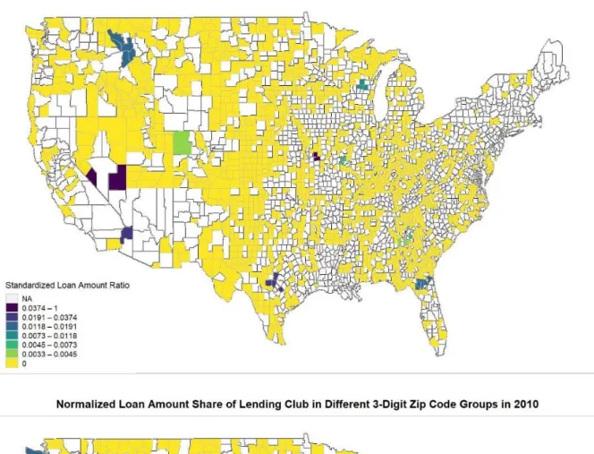
Before deeper analysis, I firstly make several heat maps to display the expand of LendingClub and its normalized loan amount share in the small business loan market, as it is shown in Figure 1. The map is color-coded based on the normalized ratio of the LendingClub loan amount to the total loan amount of LendingClub and bank. The normalized ratio is calculated by dividing the ratio of LendingClub in each sample by the maximum ratio of LendingClub in each year. The purpose of normalization is to make the ratio in different years comparable. The greater the normalized ratio, the deeper the color in that region. Yellow region means there are no LendingClub small business loans in that area, while the white region means the data in that area is not included in the analysis because of the unmatched FIPS code and zip code problem. From the graphs, we can see that there are some areas where LendingClub started and remained a high share of the market, which are the regions that have deep blue colors from 2007 to 2017. To understand the story, I figure out which counties these areas represent and make an average of its normalized loan amount ratio from 2007 to 2017. The top 20 counties are listed as Table 1.

13_{Percent Urban and Rural In 2010 by State and County, from List of Population, Land Area, and Percent Urban and}

Rural in 2010 and Changes from 2000 to 2010: https://www.census.gov/programs-surveys/geography/guidance/geo-areas/urban-rural/2010-urban-rural.html

(18)

15

Table 1. Top 20 Counties of the Share of LendingClub

According to Table 1, the top three counties are in Nevada and Arizona, areas that are close to Las Vegas. This phenomenon brings an interesting question, why counties close to Las Vegas tend to

have a high share of LendingClub? According to Census Bureau’s Quick Facts14_{and Wikipedia,}

Esmeralda County is developed by its gold mining industry and has only 783 population in 2010,

Lincoln County is the 7th-largest county in area in the U.S. and has a very low population density,

only 0.5 per square mile, while La Paz County is the 2nd-least populous county in Arizona. The

large rural area makes more difficult the access to bank services. Besides, people in Las Vegas also are also driven by the gambling preferences and have higher pressure of subprime mortgage liquidation due to gambling. Therefore, people there may provide every reason they can make up (including “financing their business”) on P2P lending platform in order to get the money to pay back their debts. The false information provided by borrowers may contribute to the extraordinary high share of LendingClub near Las Vegas.

14_{Census Bureau Quick Facts of Esmeralda, La Paz, and Lincoln County: https://www.census.gov/quickfacts/fact/} table/esmeraldacountynevada,lapazcountyarizona,lincolncountynevada,US/PST045218

Ranking FIPS code County Name State Name Average Normalized Amount Ratio

1 32009 Esmeralda County Nevada 0.8879

2 32017 Lincoln County Nevada 0.8879

3 04012 La Paz County Arizona 0.3258

4 12049 Hardee County Florida 0.0918

5 06005 Amador County California 0.0832

6 27085 McLeod County Minnesota 0.0786

7 12093 Okeechobee County Florida 0.0753

8 51049 Cumberland County Virginia 0.0664

9 06109 Tuolumne County California 0.0622

10 53059 Skamania County Washington 0.0597

11 53069 Wahkiakum County Washington 0.0597

12 48321 Matagorda County Texas 0.0591

13 48481 Wharton County Texas 0.0591

14 48099 Coryell County Texas 0.0514

15 42127 Wayne County Pennsylvania 0.0486

16 48097 Cooke County Texas 0.0480

17 48337 Montague County Texas 0.0480

18 02060 Bristol Bay Borough Alaska 0.0426

19 02282 Yakutat City and Borough Alaska 0.0426

(19)

16

(20)

17 (Figure 1 Continued)

(21)

18 Tabl e 2. Su m m ar y S ta tist ic s In ter n et Per Ho u seh o ld ( 3 -d ig it z ip co d e) C h an g e o f B an k B ran ch ( 3 -d ig it z ip co d e) B an k Den sity ( 3 -d ig it z ip co d e) Po p u latio n Den sity ( p er m illi o n sq u ar e m ile) ( 3 -d ig it z ip c o d e ) L o g o f I n co m e (3 -d ig it z ip c o d e) Un em p lo y m en t Rate (3 -d ig it z ip co d e) Ma le R atio ( 3 -d ig it z ip co d e) W h ite R atio ( 3 -d ig it z ip co d e) Ind epe nd e nt Va ria ble No rm alize d lo an n u m b er s h ar e o f L en d in g C lu b (3 -d ig it z ip co d e) No rm alize d lo an a m o u n t sh ar e o f L en d in g C lu b (3 -d ig it z ip co d e) Depende nt Va ria ble Var iab les 4 ,2 0 3 4 ,2 0 3 4 ,2 0 3 4 ,2 0 3 4 ,2 0 0 4 ,2 0 3 4 ,2 0 3 4 ,2 0 3 4 ,2 0 3 4 ,2 0 3 N (1 ) 0 .5 9 8 -0 .0 0 9 4 2 0 .2 4 4 0 .0 0 0 2 5 6 2 0 .8 7 0 .6 3 3 0 .4 9 9 0 .8 5 7 0 .0 1 9 1 0 .0 0 9 2 5 M ea n (2 ) 0 -0.2 0 0 0 .0 0 0 1 4 4 1 .4 6 e-07 1 7 .2 7 0 .4 23 0 .4 5 6 0 .2 82 0 0 M in (3₎ 1 .2 0 0 0 .2 2 2 2 2 .7 7 0 .0 2 5 1 24_.9 9 0 .8 7 9 0 .5 9 5 0 .9 9 1 1 1 M ax (4) 0 .1 5 4 0 .0 2 5 8 1 .4 7 0 0 .0 0 1 3 5 1 .1 8 0 0 .1 0 7 0 .0 1 5 1 0 .1 3 8 0 .0 7 3 3 0 .0 5 8 8 SD (5 ) 0 .3 3 0 -0 .0 5 7 4 0 .0 0 3 1 5 3 .4 5 e-06 1 8 .8 7 0 .4 6 1 0 .4 8 1 0 .5 5 5 0 0 P5 (6 ) 0 .4 2 0 -0 .0 4 0 4 0 .0 0 5 5 9 6 .4 2e -06 1 9 .3 6 0 .5 1 0 0 .4 8 4 0 .6 5 1 0 0 P 1 0 (7₎ 0 .5 0 0 -0 .0 2 2 1 0 .0 1 7 4 1 .9 9 e-05 2 0 .0 7 0 .5 7 7 0 .4 9 1 0 .8 0 7 0 0 P 2 5 (8₎ 0 .5 0 0 -0 .0 2 2 1 0 .0 1 7 4 1 .9 9 e-05 2 0 .0 7 0. 6 4 5 0 .4 9 1 0 .8 0 7 0 0 M ed ian (9₎ 0 .7 0 0 0 0 .0 9 1 6 0 .0 0 0 1 1 2 2 1 .6 8 0 .7 0 0 0 .5 0 5 0 .9 5 1 0 .0 0 9 6 0 0 .0 0 2 2 0 P 7 5 (1 0 ) 0 .7 7 0 0 .0 1 6 7 0 .2 0 1 0 .0 0 0 2 3 2 2 2 .2 9 0 .7 4 6 0 .5 1 5 0 .9 6 7 0 .0 4 1 7 0 .0 1 1 2 p90 (1 1 ) 0 .8 9 0 0 .0 2 7 8 0 .4 1 6 0 .0 0 0 5 4 3 2 2 .6 1 0 .7 8 4 0 .5 2 6 0 .9 7 5 0 .0 9 0 4 0 .0 2 9 1 P 9 5 (1 2 )

(22)

19

In addition, I also find that among the top 10 counties, two are in California and near San Francisco. This can be explained by the fact that LendingClub was founded in San Francisco and located the headquarter there. From top 10 to top 20, five counties are in Texas. Among them, two are located near Houston and three are close to Dallas. As we know, Houston is the fourth most populous city

in the United States while Dallas is the ninth.15_{Besides, Houston and Dallas are important business}

centers in the United States. Houston16_{has the second most Fortune 500 headquarters while}

Dallas17_{is the third most popular cities for business travel in the US. The industrial environment}

produces demands for start-up capitals and cultivates the growth of the small business.

The above analyses reveal the possibility that local environment and activities are important indicators for the expansion of LendingClub small business loans. The phenomenon that the top 20 counties with a high share of LendingClub tend to locate near Las Vegas, San Francisco, Dallas and Huston illustrate the theory. In addition, another crucial fact is that all 20 counties do not have big cities, but just near big cities. This may imply that small business borrowers in rural areas have more tendency to apply for loans through P2P lending than their counterparts in urban areas. Further analysis will prove whether these hypotheses are correct.

5. Empirical Results

5.1 Description Analysis

I further explore the factors that may influence the expansion of LendingClub with regression analysis, using data from LendingClub, FFIEC CRA bank loan data, and other data sources. Since the borrower’s address reported on the LendingClub dataset is limited to the 3-digit zip code, and

the borrower’s address reported on bank dataset is FIPS code18_{, I cannot match the two datasets}

directly. I only include counties that have unique 3-digit zip code (that are 467 3-digit zip code

15_{Reference: Top 50 Cities in the U.S. by Population and Rank,} https://www.infoplease.com/us/us-cities/top-50-cities-us-population-and-rank

16_{Huston Wikipedia: https://en.wikipedia.org/wiki/Houston}

17_{Dallas Wikipedia: https://en.wikipedia.org/wiki/Dallas#cite_note-:2-9}

18_{Unlike zip code, FIPS code can uniquely identify counties and county equivalents in the United States. There are}

about 3000 FIPS code on total, each FIPS code can match to one or more than one zip codes. We find that 1654 FIPS codes have unique 3-digit zip code and only include those counties into our analysis, which are equivalent to 467 3-digit zip code.

(23)

20

groups from about 900 digit zip codes). I calculate all the independent variables in the 467 3-digit zip code groups accordingly.

The dependent variables that I put into the multiple regression analysis are as follows,

1) Normalized loan amount share of LendingClub in the 3-digit zip code. Calculated as the loan amount share of LendingClub divided by the maximum loan amount share of LendingClub for each year separately. Loan amount share of LendingClub is the loan amount of LendingClub divided by the sum of the loan amount of LendingClub and the loan amount of banks.

2) Normalized loan number share of LendingClub in the 3-digit zip code. Calculated as the loan number share of LendingClub divided by the maximum loan number share of LendingClub for each year separately. Loan number share of LendingClub is the loan number of LendingClub divided by the sum of the loan number of LendingClub and the loan number of banks.

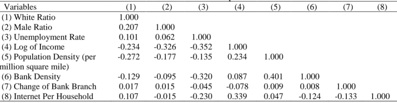
Table 2 is the summary statistics of the variables I include in the regression analysis. From the quantiles of the dependent variables, I find that the dependent variables follow the skewed distribution and most of the samples are zero, which may lead to a weak relationship between dependent variables and independent variables. To avoid this problem, I make ordinary multiple regressions first and then conduct quantile regression to focus more on the samples whose dependent variables are not zero. I delete 3 samples whose income are zero and the final sample size is 4200. Table 3 is the correlation matrix of the independent variables.

Table 3. Correlation Matrix of Independent Variables

Variables (1) (2) (3) (4) (5) (6) (7) (8) (1) White Ratio 1.000

(2) Male Ratio 0.207 1.000

(3) Unemployment Rate 0.101 0.062 1.000

(4) Log of Income -0.234 -0.326 -0.352 1.000 (5) Population Density (per

million square mile)

-0.272 -0.177 -0.135 0.234 1.000

(6) Bank Density -0.129 -0.095 -0.320 0.087 0.401 1.000

(7) Change of Bank Branch 0.017 0.015 -0.045 -0.078 0.009 0.008 1.000

(24)

21

Figure 2. Scatter Plots between Normalized Loan Amount Share of LendingClub in 3-Digit Zip Code and Independent Variables

AmountRatioST is the normalized loan amount share of LendingClub. I only draw the scatter plot of AmountRatioST and the independent variables because I consider this variable as the main dependent variable.

To understand the relationship between dependent variables and independent variables better, I draw the scatter plots between normalized loan amount share of LendingClub and all the independent variables before the regression analysis, as Figure 2 demonstrates.

5.2 Ordinary Least Square Regression

5.2.1 Univariate Regression

Before multiple regression analysis, I conduct univariate regression between the dependent variable and each independent variable separately, as Table 4.1 and Table 4.2 show. Since the sample is based on 3-digit zip code group, I adjust the cluster effect of 3-digit zip code (Parente and Santos Silva, 2016). Since the laws and policies concerning peer-to-peer lending and small business may differ across states, I include a series of dummies indicating which state the region is located to control for the difference between states. I use the Nevada state as the reference state,

(25)

22

where the top 2 shares of LendingClub counties locate. I also include dummy variables of the year to control the time effect.

Table 4.1 Univariate Regression Results: Relation Between the Normalized Loan Amount Share of LendingClub in 3-Digit Zip Code and Independent Variables

Column 1 to 8 are the univariate regression results of the normalized share of LendingClub concerning loan amount accordingly. I summarize each variable on a 3-digit zip code base in each year and consider the cluster effect when building the model. I include state name as dummy variables and set state NE as reference. I also include year dummies to adjust year effects. The *, **, *** represent statistical significance at 0.05, 0.01 and 0.001 respectively.

Model1 Model2 Model3 Model4 Model5 Model6 Model7 Model8 (1) (2) (3) (4) (5) (6) (7) (8) White Ratio (3-digit zip

code)

0.0056 (0.0097)

Male Ratio (3-digit zip code)

0.3135 (0.1729)

Unemployment Rate (3-digit zip code)

0.0544 (0.0283)

Log of Income (3-digit zip code)

-0.0086** (0.0030)

Population Density (per million square mile) (3-digit zip code)

-0.1546 (0.3090)

Bank Density (3-digit zip code)

0.0014*** (0.0003)

Change of Bank Branch (3-digit zip code)

0.0103 (0.0337)

Internet Per Household (3-digit zip code)

-0.0363** (0.0144) Intercept -0.0016 (0.0112) -0.1516 (0.0864) -0.0265 (0.0178) 0.1776** (0.0595) 0.0038 (0.0036) 0.0038 (0.0036) 0.0036 (0.0034) 0.0212** (0.0068)

State Fixed Effects Yes Yes Yes Yes Yes Yes Yes Yes

Year Fixed Effects Yes Yes Yes Yes Yes Yes Yes Yes

Number of Observations 4203 4203 4203 4200 4203 4203 4203 4203

r2 0.1260 0.1304 0.1328 0.1495 0.1259 0.1269 0.1259 0.1317

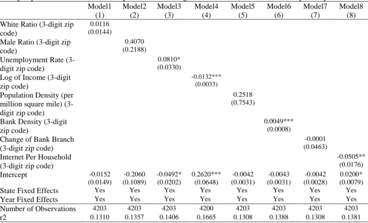
Univariate regression reveals that the unemployment rate is positively related to the share of LendingClub, as column 2 in table 4.2 shows. Income has a negative influence on the share of LendingClub, as column 3 in table 4.1 and table 4.2 indicate. The coefficients of the two variables are consistent with our hypothesis. Bank density has a positive influence on the share of LendingClub, however, is inconsistent with our hypothesis. This means that where bank density is higher, the share of LendingCLub is higher. The negative coefficient of internet coverage is not consistent with our hypothesis either. I get a more comprehensive understanding of this relationship through multiple regression.

(26)

23

Table 4.2 Univariate Regression Results: Relation Between the Normalized Loan Number Share of LendingClub in 3-Digit Zip Code and Independent Variables

Column 1 to 8 are the univariate regression results of the normalized share of LendingClub concerning loan number accordingly. I summarize each variable on a 3-digit zip code base in each year and consider the cluster effect when building the model. I include state name as dummy variables and set state NE as reference. I also include year dummies to adjust year effects. The *, **, *** represent statistical significance at 0.05, 0.01 and 0.001 respectively.

Model1 Model2 Model3 Model4 Model5 Model6 Model7 Model8 (1) (2) (3) (4) (5) (6) (7) (8) White Ratio (3-digit zip

code)

0.0116 (0.0144)

Male Ratio (3-digit zip code)

0.4070 (0.2188)

Unemployment Rate (3-digit zip code)

0.0810* (0.0330)

Log of Income (3-digit zip code)

-0.0132*** (0.0033)

0.2518 (0.7543)

Bank Density (3-digit zip code)

0.0049*** (0.0008)

-0.0001 (0.0463)

Internet Per Household (3-digit zip code)

-0.0505** (0.0176) Intercept -0.0152 (0.0149) -0.2060 (0.1089) -0.0492* (0.0202) 0.2620*** (0.0648) -0.0042 (0.0031) -0.0043 (0.0031) -0.0042 (0.0028) 0.0200* (0.0079)

State Fixed Effects Yes Yes Yes Yes Yes Yes Yes Yes

Year Fixed Effects Yes Yes Yes Yes Yes Yes Yes Yes

Number of Observations 4203 4203 4203 4200 4203 4203 4203 4203

r2 0.1310 0.1357 0.1406 0.1665 0.1308 0.1388 0.1308 0.1381

5.2.2 Multiple Regression

To understand why bank density is positively related to the share of LendingClub, I need to know if there are other factors that may be related to bank density and I did not take into consideration. Maybe the positive coefficient is caused by the endogeneity problem. Therefore, I include a dummy variable indicating whether the region is in an urban area or in a rural area, Urban. I also consider the cluster effect of 3-digit zip code and the state dummies in the multiple regression model.

The results from column 1 and 2 in Table 5 are almost the same. The coefficient of income indicates that the local average income can significantly decrease the share of LendingClub (p<0.01). In other words, small business owners in regions with lower income will have more tendency to get their start-up capitals through LendingClub and other online peer-to-peer lending

(27)

24

platforms, instead of going to the banks. This shows that LendingClub has more market share in areas where local economies are less developed.

Table 5. Multiple Regression Results: Relation Between the Share of LendingClub in 3-Digit Zip Code and Independent Variables

Column 1 and 2 are the results of the normalized share of LendingClub concerning loan amount and loan number accordingly. I summarize each variable on a 3-digit zip code base in each year and consider the cluster effect when building the model. I include state name as dummy variables and set state NE as reference, the states in the sample are AK, AL, AR, AZ, CA, CO, CT, DE, FL, GA, HI, IA, ID, IL, IN, KS, KY, LA, MA, MD, MI, MN, MO, MS, MT, NC, ND, NE, NH, NJ, NM, NV, NY, OH, OK, OR, PA, RI, SC, SD, TN, TX, UT, VA, VT, WA, WI, WV and WY. I also include year dummies. Only states and years with significant effects are displayed in the table below. The *, **, *** represent statistical significance at 0.05, 0.01 and 0.001 respectively.

Normalized loan amount share of LendingClub in 3-digit zip

code

Normalized loan number share of LendingClub in 3-digit zip

code

(1) (2)

White Ratio (3-digit zip code) -0.0102 (0.0099) -0.0139 (0.0147) Male Ratio (3-digit zip code) 0.1178 (0.1580) 0.0925 (0.2055) Unemployment Rate (3-digit zip

code)

0.0155 (0.0178) 0.0381 (0.0212) Log of Income (3-digit zip code) -0.0072**_(0.0024) _-0.0111***_(0.0028)

0.4540 (0.5169) -0.0160 (0.6382) Bank Density (3-digit zip code) 0.0019**_(0.0006) _0.0061***_(0.0008)

0.0043 (0.0323) -0.0095 (0.0443) Internet Per Household (3-digit

zip code)

-0.0134 (0.0087) -0.0168 (0.0124) Urban (3-digit zip code) -0.0051 (0.0041) -0.0054 (0.0053) Year 2010 -0.0000 (0.0042) 0.0091*_(0.0044) Year 2013 -0.0032 (0.0042) 0.0342***_(0.0054) CA 0.0290***_(0.0080) _0.0555***_(0.0156) CT 0.0135**_(0.0045) _0.0267***_(0.0066) DE 0.0133*_(0.0055) _0.0228**_(0.0080) FL 0.0238**_(0.0087) _0.0415**_(0.0140) GA 0.0086 (0.0053) 0.0222*_(0.0090) HI 0.0156 (0.0089) 0.0362**_(0.0118) IN 0.0067 (0.0041) 0.0137*_(0.0061) MI 0.0063 (0.0053) 0.0214*_(0.0086) NJ 0.0080 (0.0043) 0.0396***_(0.0065) OH 0.0140 (0.0073) 0.0208**_(0.0068) OR 0.0101 (0.0055) 0.0204*_(0.0090) PA 0.0086 (0.0057) 0.0172*_(0.0068) RI 0.0174**_(0.0054) _0.0314***_(0.0075) SC 0.0067 (0.0073) 0.0232*_(0.0097) TX 0.0113*_(0.0048) _0.0217**_(0.0081) UT 0.0092 (0.0053) 0.0215**_(0.0080) VA 0.0068 (0.0048) 0.0172*_(0.0082) VT 0.0113 (0.0066) 0.0219*_(0.0094) WA 0.0096 (0.0061) 0.0344*_(0.0165) Intercept 0.1026 (0.0834) 0.1783 (0.1080)

State Fixed Effects Yes Yes

Year Fixed Effects Yes Yes

Number of Observations 4200 4200

(28)

25

Nevertheless, the result also shows that bank density can increase the share of LendingClub, which is different from our hypothesis (p<0.01). I think there may be the high correlation between bank density and population density and calculate the variance inflation factor of the model. Results show that the VIFs of bank density and population density are smaller than 2. Therefore, I cannot explain this by multicollinearity. One explanation is LendingClub and the bank are complements and the share of LendingClub will increase in regions where bank branches are densely distributed. Another explanation is the regions where bank density is high are usually urban areas with the more developed economic environment and have more small and medium-sized enterprises. I conduct robustness test in the first part of section 6 to test this.

In addition, race, gender, unemployment rate, population density, change of bank branch and Internet coverage do not show any significant relation with the share of LendingClub. Quantile regression in the next section can separate the effects to explore the relation more easily. The insignificant result of Internet coverage is reasonable because high Internet coverage can not only promote the use of the peer-to-peer lending platform but also promote the use of the online services of banks. Future studies should find a better indicator to separate these two effects. Moreover, from the results of the year dummy, I can find that the share of LendingClub concerning loan number is increasing over the past ten years. This tendency is also consistent with the heat map.

5.3 Quantile Regression

The summary statistics in Table 2 shows that the dependent variables are not distributed evenly and there are so many zeros. To better explore what affects the share of LendingClub, I conduct quantile regression for each dependent variable. The clustered effect of 3-digit zip code and state dummies are also taken into consideration in the analysis.

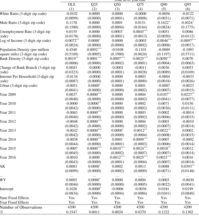
The result of quantile regression reveals more details as table 6.1 and table 6.2 illustrate. Take table 6.1 as an example, at high quantiles of the share of LendingClub, regions with a higher ratio of male have a higher share of LendingClub (Column 5,6, p<0.05), which is consistent with our hypothesis. The unemployment rate is significantly positively related to the share of LendingClub (Column 4,5) demonstrates that LendingClub has a higher share of the market where the unemployment rate is high. This is also consistent with our hypothesis. Income has a negative

(29)

26

Table 6.1 Ordinary Least Squares and Quantile Regressions of Normalized Loan Amount Share of LendingClub in 3-Digit Zip Code

Column 1 is the multiple regression results of the normalized loan amount ratio of LendingClub. Column 2 to 6 is the quantile regression results at 25 percent, 50 percent, 75 percent, 90 percent, and 95 percent. I summarize each variable on a 3-digit zip code base in each year and consider the cluster effect when building the model. I include state name as dummy variables and set state NE as reference, the states in the sample are AK, AL, AR, AZ, CA, CO, CT, DE, FL, GA, HI, IA, ID, IL, IN, KS, KY, LA, MA, MD, MI, MN, MO, MS, MT, NC, ND, NE, NH, NJ, NM, NV, NY, OH, OK, OR, PA, RI, SC, SD, TN, TX, UT, VA, VT, WA, WI, WV and WY. The results for states are omitted. I also include year dummies. Only years with significant effects are displayed in the table below. The *, **, *** represent statistical significance at 0.05, 0.01 and 0.001 respectively.

Normalized ratio of LendingClub loan amount to the total loan amount in 3-digit zip code as of year-end

OLS Q25 Q50 Q75 Q90 Q95

(1) (2) (3) (4) (5) (6)

White Ratio (3-digit zip code) -0.0102 (0.0099) 0.0000 (0.0000) 0.0000 (0.0001) -0.0000 (0.0008) -0.0056 (0.0031) -0.0122 (0.0071) Male Ratio (3-digit zip code) 0.1178

(0.1580) 0.0000 (0.0000) 0.0001 (0.0004) 0.0151 (0.0164) 0.1622* (0.0824) 0.4024* (0.1775) Unemployment Rate (3-digit zip

code) 0.0155 (0.0178) 0.0000 (0.0000) 0.0003* (0.0001) 0.0045*** (0.0013) 0.0051 (0.0050) 0.0086 (0.0112) Log of Income (3-digit zip code) -0.0072**

(0.0024) 0.0000* (0.0000) 0.0000 (0.0000) -0.0003 (0.0002) -0.0046*** (0.0008) -0.0097*** (0.0017) Population Density (per million

square mile) (3-digit zip code)

0.4540 (0.5169) 0.0092*** (0.0005) -0.0108 (0.1980) -0.1101 (0.0626) -0.0889 (0.1197) -0.1093 (0.5711) Bank Density (3-digit zip code) 0.0019**

(0.0006) 0.0001*** (0.0000) 0.0007*** (0.0002) 0.0025*** (0.0001) 0.0050*** (0.0004) 0.0070 (0.0063) Change of Bank Branch (3-digit zip

code) 0.0043 (0.0323) -0.0000 (0.0000) -0.0001 (0.0001) -0.0011 (0.0028) 0.0036 (0.0089) 0.0053 (0.0169) Internet Per Household (3-digit zip

code) -0.0134 (0.0087) -0.0000 (0.0000) 0.0000 (0.0001) 0.0003 (0.0009) -0.0004 (0.0018) -0.0033 (0.0026) Urban (3-digit zip code) -0.0051

(0.0041) 0.0000* (0.0000) 0.0000 (0.0000) 0.0001 (0.0002) -0.0007 (0.0007) -0.0023 (0.0015) Year 2009 0.0037 (0.0040) 0.0000*** (0.0000) 0.0000 (0.0000) 0.0004 (0.0002) 0.0107** (0.0041) 0.0227** (0.0077) Year 2010 -0.0000 (0.0042) 0.0000** (0.0000) 0.0000 (0.0000) 0.0002 (0.0002) 0.0071 (0.0036) 0.0156 (0.0111) Year 2011 -0.0063 (0.0040) 0.0000*** (0.0000) 0.0000 (0.0000) 0.0003 (0.0002) 0.0002 (0.0006) -0.0014 (0.0015) Year 2012 -0.0048 (0.0042) 0.0000*** (0.0000) 0.0000 (0.0000) 0.0004 (0.0002) 0.0003 (0.0007) -0.0010 (0.0014) Year 2013 -0.0032 (0.0042) 0.0000*** (0.0000) 0.0000* (0.0000) 0.0012** (0.0004) 0.0022** (0.0008) 0.0002 (0.0015) Year 2014 -0.0038 (0.0044) 0.0000*** (0.0000) 0.0001 (0.0001) 0.0009*** (0.0003) 0.0007 (0.0006) -0.0002 (0.0014) Year 2015 -0.0007 (0.0045) 0.0000*** (0.0000) 0.0010*** (0.0002) 0.0024*** (0.0007) 0.0018** (0.0007) 0.0012 (0.0014) Year 2016 -0.0010 (0.0043) 0.0000 (0.0000) 0.0012*** (0.0001) 0.0025*** (0.0004) 0.0023*** (0.0007) 0.0016 (0.0014) AK 0.0083 (0.0099) 0.0000* (0.0000) 0.0002 (0.0002) 0.0013 (0.0009) 0.0088 (0.0071) 0.0393** (0.0148) … … … … WY 0.0003 (0.0046) 0.0000* (0.0000) 0.0000 (0.0000) 0.0004 (0.0005) 0.0003 (0.0022) -0.0030 (0.0041) Intercept 0.1026 (0.0834) -0.0000* (0.0000) -0.0006 (0.0004) -0.0036 (0.0086) 0.0181 (0.0361) 0.0199 (0.0840)

State Fixed Effects Yes Yes Yes Yes Yes Yes

Year Fixed Effects Yes Yes Yes Yes Yes Yes

Number of Observations 4200 4200 4200 4200 4200 4200

(30)

27

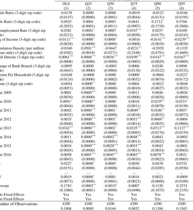
Table 6.2 Ordinary Least Squares and Quantile Regressions of Normalized Loan Number Share of LendingClub in 3-Digit Zip Code

Column 1 is the multiple regression results of the normalized loan number ratio of LendingClub. Column 2 to 6 is the quantile regression results at 25 percent, 50 percent, 75 percent, 90 percent, and 95 percent. I summarize each variable on a 3-digit zip code base in each year and consider the cluster effect when building the model. I include state name as dummy variables and set state NE as reference, the states in the sample are AK, AL, AR, AZ, CA, CO, CT, DE, FL, GA, HI, IA, ID, IL, IN, KS, KY, LA, MA, MD, MI, MN, MO, MS, MT, NC, ND, NE, NH, NJ, NM, NV, NY, OH, OK, OR, PA, RI, SC, SD, TN, TX, UT, VA, VT, WA, WI, WV and WY. The results for states are omitted. I also include year dummies. Only years with significant effects are displayed in the table below. The *, **, *** represent statistical significance at 0.05, 0.01 and 0.001 respectively.

Normalized ratio of LendingClub loan number to the total loan amount in 3-digit zip code as of year-end

OLS Q25 Q50 Q75 Q90 Q95

(1) (2) (3) (4) (5) (6)

White Ratio (3-digit zip code) -0.0139 (0.0147) 0.0000 (0.0000) 0.0000 (0.0001) -0.0019 (0.0044) -0.0123 (0.0131) -0.0166 (0.0195) Male Ratio (3-digit zip code) 0.0925

(0.2055) 0.0001 (0.0001) 0.0003 (0.0011) 0.0441 (0.0907) 0.3712* (0.1710) 0.5766 (0.3860) Unemployment Rate (3-digit zip

code) 0.0381 (0.0212) 0.0001* (0.0000) 0.0007 (0.0004) 0.0187*** (0.0050) 0.0257 (0.0175) 0.0109 (0.0243) Log of Income (3-digit zip code) -0.0111***

(0.0028) 0.0000* (0.0000) 0.0000* (0.0000) -0.0016 (0.0008) -0.0141*** (0.0029) -0.0239*** (0.0038) Population Density (per million

-0.0160 (0.6382) 0.0501*** (0.0018) -0.0447 (0.0271) -0.8231** (0.2548) -0.5929 (0.4791) -0.1335 (0.4669) Bank Density (3-digit zip code) 0.0061***

(0.0008) 0.0006*** (0.0000) 0.0026*** (0.0000) 0.0109*** (0.0003) 0.0147*** (0.0029) 0.0167*** (0.0009) Change of Bank Branch (3-digit zip

code) -0.0095 (0.0443) 0.0000 (0.0000) -0.0003 (0.0004) 0.0006 (0.0136) 0.0248 (0.0322) 0.0098 (0.0532) Internet Per Household (3-digit zip

code) -0.0168 (0.0124) -0.0000 (0.0000) 0.0000 (0.0002) 0.0009 (0.0032) -0.0066 (0.0074) -0.0237 (0.0172) Urban (3-digit zip code) -0.0054

(0.0053) 0.0000** (0.0000) 0.0000 (0.0000) 0.0004 (0.0010) -0.0023 (0.0027) -0.0048 (0.0032) Year 2009 0.0001 (0.0036) 0.0000*** (0.0000) 0.0000 (0.0000) 0.0011 (0.0006) 0.0046 (0.0026) -0.0026 (0.0069) Year 2010 0.0091* (0.0044) 0.0000** (0.0000) 0.0000 (0.0000) 0.0018 (0.0011) 0.0235** (0.0078) 0.0333* (0.0158) Year 2011 0.0042 (0.0035) 0.0000*** (0.0000) 0.0001* (0.0000) 0.0049** (0.0018) 0.0106** (0.0032) 0.0057 (0.0072) Year 2012 0.0035 (0.0040) 0.0000*** (0.0000) 0.0001* (0.0000) 0.0051*** (0.0014) 0.0069** (0.0025) -0.0004 (0.0066) Year 2013 0.0342*** (0.0054) 0.0000*** (0.0000) 0.0001* (0.0000) 0.0335*** (0.0083) 0.0713*** (0.0176) 0.1127*** (0.0159) Year 2014 0.0011 (0.0044) 0.0000*** (0.0000) 0.0002*** (0.0001) 0.0048*** (0.0013) 0.0043 (0.0022) -0.0003 (0.0061) Year 2015 0.0034 (0.0045) 0.0000*** (0.0000) 0.0028*** (0.0005) 0.0053*** (0.0013) 0.0043 (0.0024) -0.0001 (0.0062) Year 2016 0.0058 (0.0043) 0.0001*** (0.0000) 0.0045*** (0.0008) 0.0083*** (0.0010) 0.0078*** (0.0023) 0.0021 (0.0065) AK 0.0227 (0.0151) 0.0000* (0.0000) 0.0005 (0.0008) 0.0050 (0.0044) 0.0470 (0.0285) 0.0752 (0.0556) … … … .. WY 0.0019 (0.0073) 0.0000* (0.0000) 0.0001 (0.0001) 0.0016 (0.0023) 0.0023 (0.0068) -0.0009 (0.0109) Intercept 0.1783 (0.1080) -0.0003** (0.0001) -0.0015* (0.0008) 0.0007 (0.0490) 0.1120 (0.1075) 0.2574 (0.2155)

State Fixed Effects Yes Yes Yes Yes Yes Yes

Year Fixed Effects Yes Yes Yes Yes Yes Yes

Number of Observations 4200 4200 4200 4200 4200 4200

(31)

28

influence on the share of LendingClub at high quantiles means lower income regions will have more small business entrepreneurs borrow money from LendingClub (Column 5,6, p<0.001). Population density has a significantly positive influence on the share of LendingClub at low quantile (column 2) and has a negative influence on the share of LendingClub at high quantiles, though insignificant (column 3 to 6). This is reasonable because, in regions where LendingClub just enters the market, higher population density means lower learning costs (Havrylchyk et al., 2018), thus easier access to the online peer-to-peer platform. In regions where LendingClub has already have a relatively higher share of the market, high population density, however, means more economically developed in these areas, thus more bank competitors and lower share of the market. Bank density is significantly positively related to the share of LendingClub even though the urban dummy and state difference are taken into consideration. I may explain this by endogeneity or the bank and LendingClub as complements. The result that Internet per household has insignificantly influence on the share of LendingClub makes sense because both bank and LendingClub have online service, and I cannot proxy high Internet coverage as the advantage of LendingClub. In a short summary, the results of quantile regression are consistent with our hypotheses except for bank density. I will conduct robustness test to further explore it.

6. Robustness test

6.1 Coefficient of Bank Density

I add two variables, the number of small business and House Price Index (HPI) into the original multiple regression to explore further about the coefficient of bank density.

Firstly, I have reasons to believe that the regions where bank density is higher may have more investment opportunities brought by small business, thus, the number of small business in the region is higher accordingly. The relation between bank density and small business distribution may cause an endogeneity problem and lead to a “false” positive relation between bank density and the share of LendingClub. Therefore, I include the number of small business as a proxy for small business market concentration. The data is downloaded from the Census Bureau’s County

(32)

29

Business Patterns dataset19_{. I define the small business as companies with fewer than 250}

employees according to the definition of small business in the United States20_{. The data is}

summarized in 3-digit zip code groups.

Besides, to adjust the economic environment between different regions better, I include the House Price Index (HPI). HPI is an indicator of the local economy as much previous literature proved (Haurin and Hendershott, 1991; Jagtiani and Lemieux, 2018; Miller et al., 2011). The data of HPI

is obtained from the Federal House Financing Agency21_{in 3-digit zip code groups. The missing}

data of 3-digit zip code “248” is replaced by “247”.

Table 6 lists the correlation coefficients between the independent variables. I find that small business number and HPI is relatively highly correlated with income. To avoid multicollinearity problem, I estimate the variance inflation factors for each model and find no multicollinearity in the models.

Table 6. Correlation Matrix of Independent Variables

Variables (1) (2) (3) (4) (5) (6) (7) (8) (9) (10)

(1) White Ratio 1.000

(2) Male Ratio 0.207 1.000

(3) Unemployment Rate 0.101 0.062 1.000

(4) Log of Income -0.234 -0.326 -0.352 1.000 (5) Population Density (per

million square mile)

-0.272 -0.177 -0.135 0.234 1.000

(6) Bank Density -0.129 -0.095 -0.320 0.087 0.401 1.000

(7) Change of Bank Branch 0.017 0.015 -0.045 -0.078 0.009 0.008 1.000

(8) Internet Per Household 0.107 -0.015 -0.230 0.339 0.047 0.080 -0.133 1.000

(9) Log of HPI -0.084 -0.028 -0.224 0.458 0.253 0.201 -0.046 0.343 1.000

(10) Log of Small Business -0.157 -0.163 -0.069 0.607 0.172 0.163 -0.140 0.360 0.605 1.000

19_{Small business data source: Census Bureau CBP dataset:}

https://www.census.gov/programs-surveys/cbp/data/datasets.html

20_{Business size definition: https://en.wikipedia.org/wiki/Small_business}

21_{FHFA house price index (HPI) data source:}

(33)

30

Table 7. Regression Results of Robustness Test: Relation Between the Normalized Amount Ratio of LendingClub in 3-Digit Zip Code and Independent Variables

The dependent variable is the normalized loan amount share of LendingClub. Column 1 is the original multiple regression of the normalized loan amount share of LendingClub, Column 2 considers small business distribution, Column 3 considers local house price index (HPI), and Column 4 takes both variables into consideration. I summarize each variable on a 3-digit zip code base in each year and consider the cluster effect when building the model. I include state name as dummy variables and set state NE as reference, the states in the sample are AK, AL, AR, AZ, CA, CO, CT, DE, FL, GA, HI, IA, ID, IL, IN, KS, KY, LA, MA, MD, MI, MN, MO, MS, MT, NC, ND, NE, NH, NJ, NM, NV, NY, OH, OK, OR, PA, RI, SC, SD, TN, TX, UT, VA, VT, WA, WI, WV and WY. I also include year dummies. Only states and years with significant effects are displayed in the table below. The *, **, *** represent statistical significance at 0.05, 0.01 and 0.001 respectively.

Model 1 Model 2 Model 3 Model 4

(1) (2) (3) (4)

White Ratio (3-digit zip code) -0.0102 (0.0099) -0.0166 (0.0100) -0.0177 (0.0104) -0.0167 (0.0100) Male Ratio (3-digit zip code) 0.1178 (0.1580) 0.1787 (0.1367) 0.1343 (0.1474) 0.1787 (0.1366) Unemployment Rate (3-digit zip

code)

0.0155 (0.0178) -0.0338 (0.0189) 0.0016 (0.0142) -0.0337 (0.0189) Log of Income (3-digit zip code) -0.0072**_(0.0024) _-0.0196**_(0.0064) _-0.0123**_(0.0041) _-0.0196**_(0.0064) Population Density (per million

0.4540 (0.5169) 0.7480 (0.5893) -0.4120 (0.4923) 0.7289 (0.6044) Bank Density (3-digit zip code) 0.0019**_(0.0006) _{-0.0012 (0.0010)} _0.0010**_(0.0004) _{-0.0012 (0.0010)} Change of Bank Branch (3-digit

zip code)

0.0043 (0.0323) -0.0093 (0.0320) -0.0017 (0.0326) -0.0094 (0.0320) Internet Per Household (3-digit

zip code)

-0.0134 (0.0087) -0.0169 (0.0087) -0.0213*_(0.0100) _-0.0170*_(0.0085) Urban (3-digit zip code) -0.0051 (0.0041) -0.0026 (0.0033) -0.0027 (0.0036) -0.0026 (0.0033) Log of Small Business (3-digit

zip code)

0.0264** (0.0093) 0.0262** (0.0095)

Log of HPI (3-digit zip code) 0.0355** (0.0133) 0.0007 (0.0049)

Year 2009 0.0037 (0.0040) 0.0047 (0.0041) 0.0054 (0.0042) 0.0048 (0.0041) Year 2010 -0.0000 (0.0042) 0.0017 (0.0045) 0.0033 (0.0049) 0.0017 (0.0045) Year 2011 -0.0063 (0.0040) -0.0040 (0.0044) -0.0017 (0.0050) -0.0039 (0.0044) Year 2012 -0.0048 (0.0042) -0.0206***_(0.0052) _{0.0004 (0.0054)} _-0.0204***_(0.0057) Year 2013 -0.0032 (0.0042) -0.0189***_(0.0050) _{0.0014 (0.0053)} _-0.0187***_(0.0054) Year 2014 -0.0038 (0.0044) -0.0192***_(0.0050) _{0.0001 (0.0053)} _-0.0190***_(0.0053) Year 2015 -0.0007 (0.0045) -0.0159***_(0.0046) _{0.0024 (0.0052)} _-0.0157**_(0.0048) Year 2016 -0.0010 (0.0043) -0.0164***_(0.0047) _{0.0006 (0.0046)} _-0.0162***_(0.0049) CA 0.0290***_(0.0080) _{-0.0015 (0.0115)} _{0.0035 (0.0113)} _{-0.0019 (0.0116)} CT 0.0135** (0.0045) -0.0181 (0.0110) 0.0002 (0.0053) -0.0181 (0.0109) DE 0.0133*_(0.0055) _{0.0073 (0.0057)} _0.0194**_(0.0064) _{0.0075 (0.0057)} FL 0.0238**_(0.0087) _{-0.0007 (0.0106)} _0.0255**_(0.0080) _{-0.0005 (0.0107)} GA 0.0086 (0.0053) -0.0011 (0.0069) 0.0165**_(0.0058) _{-0.0009 (0.0070)} IL 0.0061 (0.0051) -0.0095 (0.0080) 0.0126*_(0.0055) _{-0.0093 (0.0082)} IN 0.0067 (0.0041) -0.0011 (0.0060) 0.0141*_(0.0055) _{-0.0009 (0.0062)} KS 0.0047 (0.0041) 0.0052 (0.0045) 0.0099*_(0.0041) _{0.0053 (0.0045)} KY 0.0004 (0.0047) 0.0099 (0.0052) 0.0143**_(0.0053) _0.0101*_(0.0052) MA 0.0002 (0.0055) -0.0387**_(0.0132) _-0.0320**_(0.0111) _-0.0391**_(0.0130) MN 0.0137 (0.0079) -0.0008 (0.0066) 0.0130*_(0.0063) _{-0.0007 (0.0066)} OH 0.0140 (0.0073) 0.0066 (0.0084) 0.0209**_(0.0079) _{0.0067 (0.0082)} PA 0.0086 (0.0057) -0.0019 (0.0084) 0.0149**_(0.0054) _{-0.0017 (0.0084)} RI 0.0174**_(0.0054) _{-0.0077 (0.0081)} _{0.0032 (0.0050)} _{-0.0078 (0.0080)} TN 0.0041 (0.0047) -0.0067 (0.0086) 0.0108*_(0.0049) _{-0.0065 (0.0088)} TX 0.0113*_(0.0048) _{0.0006 (0.0065)} _0.0149***_(0.0044) _{0.0007 (0.0066)} Intercept 0.1026 (0.0834) 0.1239 (0.0796) 0.0120 (0.0691) 0.1220 (0.0838)