Development and Verification of Innovative Modelling Approaches for the Analysis of Framed Structures Subjected to Earthquake Action

(1)

Istituto Universitario di Studi Superiori di Pavia

Development and Verification of Innovative Modelling

Approaches for the Analysis of Framed Structures Subjected to

Earthquake Action

A Thesis Submitted in Partial Fulfilment of the Requirements for the Degree of Doctor of Philosophy in

EARTHQUAKE ENGINEERING AND

ENGINEERING SEISMOLOGY

Obtained in the framework of the Doctoral Programme in Understanding and Managing Extremes

by

Romain Sousa

(2)

(3)

Istituto Universitario di Studi Superiori di Pavia

Development and Verification of Innovative Modelling

Approaches for the Analysis of Framed Structures Subjected to

Earthquake Action

A Thesis Submitted in Partial Fulfilment of the Requirements for the Degree of Doctor of Philosophy in

EARTHQUAKE ENGINEERING AND

ENGINEERING SEISMOLOGY

Obtained in the framework of the Doctoral Programme in Understanding and Managing Extremes

by

Romain Sousa

Supervisors: António A. Correia, National Laboratory for Civil Engineering João Almeida, École Polytechnique Fédérale de Lausanne

Rui Pinho, University of Pavia

(4)

(5)

ABSTRACT

The last decades have witnessed significant progresses in the development of improved numerical models for structural analysis, as proven by hundreds of dissertations, theses, reports and journal papers dedicated to advanced constitutive models of materials and algorithms to model sectional, element and structural response. Nevertheless, the seismic behaviour of structures involves a number of nonlinear material and geometrical phenomena that, ultimately, are impossible to capture exhaustively in a single model. Furthermore, past studies showed that the most correct modelling options from the scientific viewpoint are sometimes challenged by experimental evidence.

This thesis intends to contribute to the ongoing effort of progressively bridging the existing gap between solid theoretical principles adopted in nonlinear modelling and experimental results from shake table or other experimental techniques. Such goal is firstly pursued through the application of a sensitivity analysis to the simulation of the dynamic behaviour of three distinct structures with distributed plasticity beam-column fibre-based elements based on Euler-Bernoulli beam theory. The latter were tested in international blind prediction challenges wherein the author and/or supervisors participated with encouraging results.

The goodness-of-fit for each approach is assessed through comparisons between numerical and experimental results in terms of lateral displacements as well as accelerations (when available), following two post-processing strategies: a more conventional one based on the error associated to the peak values measured during each record, and another using the frequency content characteristics of the entire response history. Sensitivity parameters included equivalent viscous damping, element discretization scheme, strain penetration effects, material constitutive models, numerical integration algorithms and analysis time-step size. The conclusions, which are interpreted in the light of state-of-the-practice recommendations and established theoretical frameworks, address fundamental modelling decisions for engineers and researchers. The referred sensitivity analysis identified the simulation of strain penetration effects as particularly relevant. They can significantly impact the seismic response of structures, contributing up to 40% of the overall lateral deformation of RC framed structures.

(6)

penetration effects. The model, which in its final form is implemented as a zero-length element, was developed so that it is compatible with any general fibre-based frame analysis software. In a nutshell, the element response is determined from cross-sectional fibre integration, where at each rebar the anchorage mechanism is explicitly modelled through a series of virtual integration points distributed along the anchorage length. The analysis is carried out by an algorithm that enforces both equilibrium and compatibility at every integration point, making use of a state-of-the-art bond stress-slip cyclic constitutive relation applicable to a wide variety of anchorage conditions. Therefore, features such as the expected failure mode (pullout or splitting), or parameters such as the concrete strength, embedment length, cyclic degradation, amplitude of steel strains, rebar type (plain or ribbed), transverse pressure, level of confinement and bond conditions can be explicitly modelled.

The element was implemented in a structural analysis software and its performance was assessed against several experimental tests, showing an encouraging accuracy while retaining appreciable computational efficiency.

(7)

ACKNOWLEDGEMENTS

Despite being an individual work, this thesis reflects somehow the contribution of a number of people to whom I would like to express my gratitude.

My first words are necessarily addressed to Professor Rui Pinho. He has been my mentor since I arrived to Pavia, and I will always be grateful to him for offering me the privilege to share both work and personal experiences with such a prominent and enthusiastic person. For this confidence from day one, it is my hope that I have been able to live up to his expectations.

I would like to also express my most sincere thanks to Doctors João Almeida and António Correia. They were my guiding light along these years and I am deeply acknowledged for their teachings and continuous encouragements in the pursuit of improved solutions. At the hardest hours they were always the firsts to push me forward. Above all, I am grateful for being able to preserve and reinforce the friendship with all of my supervisors, which started way before this long journey.

I take this opportunity to informally thank the National Laboratory for Civil Engineering, particularly the Earthquake Engineering and Structural Dynamic Unit for hosting me during a relevant period of the thesis. For the kindness and the exchanged experiences, I would like to thank to all the personnel of the unit, in particular to Doctors Alfredo Campos Costa, Paulo Candeias, Alexandra Carvalho and António Correia (again).

To all the friends I made in Pavia, especially to Ricardo Monteiro, Vítor Silva, Luís Sousa and Claudia Zelaschi, I am thankful for the interesting discussions and great moments spent on the streets of Pavia or in someone’s apartment. They were my second family during an important period of my life.

A special word to my family who has always accompanied me in my decisions, being the main support at the good and bad moments. I would like to address some additional words to my brother Hélder, for the interest revealed and promptitude to help at every occasion, and to my little sister Vanessa, for having received me and shared the evenings in her house during my stay in Lisbon. A final word to my little nephews for their contagious joy.

(8)

apart. Despite everything, you were always a support and an endless source of motivation. More than ever, I know that our love can only grow in the future.

Dear mother and father, my words are too little to thank you for everything you made for me. Thank you for making me feel the proudest a son can be. This humble work is dedicated to you.

(9)

“Everything should be made as simple as possible,

but not one bit simpler”

Albert Einstein, (attributed) US (German-born) physicist (1879 - 1955)

(10)

(11)

LIST OF FIGURES

Figure 1.1. Comparison between experimental results and numerical simulations submitted by the authors to different blind prediction challenges: maximum displacements for seismic motions of increasing intensity ... 1

Figure 1.2. Comparison between experimental results and numerical simulations on the

‘Concrete Column Blind Prediction Contest 2010’: maximum horizontal displacement (left) and maximum bending moment (right) (adapted from Terzic et

al. [2015]) ... 2

Figure 1.3. Contribution of different deformation mechanisms to the total lateral displacement according to Sezen and Moehle [2004] ... 4

Figure 2.1. Variation of damping with amplitude [Fang et al., 1999] ... 9

Figure 2.2. Lagomarsino’s and Satake’s damping predictor with respect to fundamental natural

period of buildings [Satake et al., 2003] ... 10

Figure 2.3. Damping ratio versus natural frequency at very low amplitude for steel (left) and RC

(right) buildings [Satake et al., 2003] ... 10

Figure 2.4. Damping predictors for RC buildings ... 11

Figure 2.5. Damping ratios at higher modes of vibration [Kareem and Gurley, 1996] ... 12

Figure 2.6 Damping ratios at higher modes considering different measurement methods [Morita and Kanda, 1996] ... 12

Figure 2.7. Variation of damping ratios with height and aspect ratio [Erwin et al., 2007] ... 13

Figure 2.8. Variation of damping ratios with natural frequency for different EVD models ... 15

Figure 2.9. Graphical representation of two common SP modelling approaches: elongated element (left) and base spring (right) ... 26

Figure 2.10. Capacity curves of a column of Structure 2 considering alternative strain penetration

options ... 27

Figure 2.11. Cyclic response of the same concrete fibre in the base section of Structure 1 using

distinct uniaxial models, for the same cyclic history of imposed lateral displacements ... 29

Figure 2.12. Cyclic response of the same reinforcement fibre in the base section of Structure 1

using distinct uniaxial models, for the same cyclic history of imposed lateral displacements ... 31

(16)

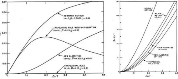
Figure 2.13. Variation of amplitude decay and period elongation with respect to Δt/T, for

different numerical integration methods (adapted from Hilber et al. [1977]) ... 32

Figure 2.14. SMART 2013 mock-up ... 34

Figure 2.15. Plan view and dimensions of the mock-up (in mm) ... 35

Figure 2.16. Numerical model with shell elements (left) and wide-column analogy (centre and right) ... 39

Figure 2.17. Ground motion considered in the numerical analyses: X (left) and Y (right) direction41

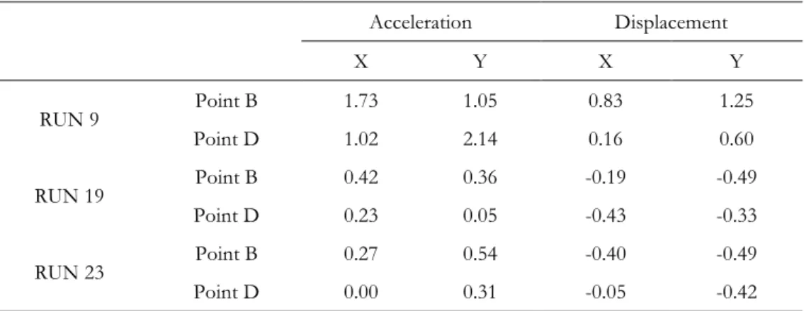
Figure 2.18. History of accelerations and displacements – RUN 19, X-direction, point B ... 42

Figure 2.19. History of accelerations and displacements – RUN 19, Y-direction, point B ... 42

Figure 2.20. History of accelerations and displacements – RUN 9, Y-direction, point B ... 43

Figure 2.21. History of accelerations and displacements – RUN 23, Y-direction, point D ... 44

Figure 3.1. Structure 1: Elevation view (left) and cross-section details (right) ... 48

Figure 3.2. 1st_{(left) and 2}nd_{(right) modal shapes of Structure 1 ... 49}

Figure 3.3. Lateral load-displacement (left) and moment-curvature (right) response of Structure 149

Figure 3.4. Series of applied acceleration records to Structure 1 ... 50

Figure 3.5. Structures 2 and 3: General dimensions of the mock-up ... 50

Figure 3.6. Beam/column joint reinforcement details of Structure 2 (left) and Structure 3 (right) 51

Figure 3.7. 1st_{(left), 2}nd_{(centre) and 4}th_{(right) modal shapes of Structure 2 ... 52}

Figure 3.8. Lateral load-displacement (left) and moment-curvature (right) response of Structure 2 along Y direction ... 53

Figure 3.9. Lateral load-displacement (left) and moment-curvature (right) response of Structure 3 along Y direction ... 53

Figure 3.10. Series of applied acceleration records on Structure 2 in the longitudinal direction ... 54

Figure 3.11. Graphical representation of the real and imaginary components of the calculated and measured quantities in the frequency domain ... 61

Figure 3.12. Outline of the parametric study ... 63

Figure 3.13. Peak displacement (left) and acceleration (right) error for Structure 1 considering different EVD models ... 64

Figure 3.14. Peak displacement error for Structures 2 (left) and 3 (right) considering different EVD models ... 64

Figure 3.15. Transverse (left) and rotational (right) history of accelerations measured in Structure 1 during Eqk 4 considering 0.5% MPD and 0.5% TSPD ... 65

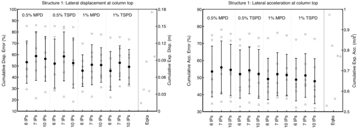
Figure 3.16. Cumulative displacement (left) and acceleration (right) error for Structure 1 considering different discretization schemes ... 66

(17)

Figure 3.17. Cumulative displacement error for Structures 2 (left) and 3 (Right), considering different discretization schemes ... 67

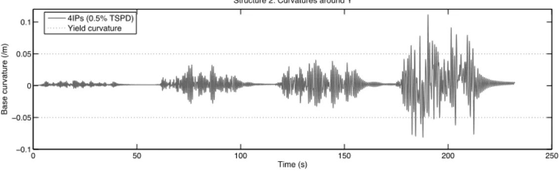
Figure 3.18. History of curvatures measured at the column base below Point B of Structure 2

considering 0.5% TSPD and 4 IPs per column ... 67

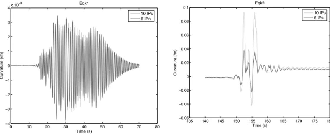
Figure 3.19. Predicted curvatures at base IP for Structure 1 during Eqk 1 and Eqk 3 ... 68

Figure 3.20. Comparison between measured and simulated displacement time-histories in

Structure 1, considering 0.5 % MPD with 6 IPs during Eqk 3 ... 69

Figure 3.21. Peak (left) and cumulative (right) displacement error for Structure 1, considering

different SP models ... 69

Figure 3.24. Time-history of measured displacements in Structure 2 (point A, direction X) vs

displacements computed with different SP models, during Eqk 1 and Eqk 3 ... 71

Figure 3.25. Peak displacement error (left) and acceleration (right) error for Structure 1 considering different concrete models ... 72

Figure 3.26. Peak displacement error for Structure 2 (left) and 3 (right) considering different

concrete models ... 73

Figure 3.27. Time-history of simulated displacements in Structure 3 (point A, direction X)

considering Mander’s concrete model with and without tensile strength ... 73

Figure 3.28. History of simulated strains in Structure 1 at diametrically opposed fibres of the

base section compressed core, for the entire set of records and considering alternative concrete models ... 74

Figure 3.29. Simulated stress-strain response in Structure 1 at diametrically opposed fibres of the

base section, for the entire set of records and considering alternative concrete models ... 75

Figure 3.30. Cumulative displacement (left) and acceleration (right) error for Structure 1

considering different steel models ... 76

Figure 3.31. Cumulative displacement error for Structure 2 (left) and 3 (right) considering

different steel models ... 76

Figure 3.32. Stress-strain response at diametrically opposed fibres of the base section (top) and

history of simulated curvatures (bottom) in Structure 1 for the entire set of records considering alternative steel models ... 77

Figure 3.33. Peak (left) and cumulative (right) displacement error for Structure 1 considering

different integration algorithms ... 78

Figure 3.34. Peak (left) and cumulative (right) displacement error for Structure 2 considering

(18)

Figure 3.35. Peak (left) and cumulative (right) displacement error for Structure 3 considering different integration algorithms ... 79

Figure 3.36. Peak (left) and cumulative (right) acceleration error for Structure 1 considering

different integration algorithms ... 79

Figure 3.37. Peak displacements error for Structure 1 considering different time-steps with HHT

(left) and Newmark (right) integration algorithms ... 80

Figure 3.38. Peak acceleration error for Structure 1 considering different time-steps, with HHT

Figure 3.39. Time-history of transversal accelerations measured in Structure 1 vs transversal

accelerations computed with HHT (left) and Newmark (right) integration algorithm and increasing time-step (top to bottom), during Eqk 3 ... 82

Figure 4.1. Behaviour of anchorage region with adequate (left) and limited (right) embedment

length (adapted from Sritharan et al. [2000]) ... 88

Figure 4.2. Lateral displacement components measured in a circular RC column (Test 9)

[Goodnight et al., 2015a] ... 89

Figure 4.3. Bond mechanisms at the anchorage region of a RC member ... 90

Figure 4.4. Influence of different transfer mechanisms in the bond-slip relations (adapted from

fib [2000] ... 92

Figure 4.5. Different typologies of anchorage failure: splitting (left) and pullout (shearing) failure

of anchorage systems [ACI, 2003] ... 92

Figure 4.6. Example of a pullout test setup [Casanova et al., 2013] ... 94

Figure 4.7. Evolution of bond strength with the concrete cover for different transverse pressure

[Casanova et al., 2013] ... 95

Figure 4.8. Bond stress-slip relation under different passive confinement conditions [Eligehausen

et al., 1983] ... 95

Figure 4.9. Bond stress-slip response under different transverse pressure [Malvar, 1991] ... 96

Figure 4.10. Evolution of maximum (left) and frictional (right) bond stress components with

transverse pressure from different studies presented by Eligehausen et al. [1983] ... 97

Figure 4.11. Evolution of bond stress with relative rib area with and without transverse reinforcement (left) and with different spacing (h) of transverse reinforcement

(right) [Darwin and Graham, 1993] (1 kips = 4448.2 N / 1 in = 0.0254 m) ... 98

Figure 4.12. Variation in the bond-slip response for different rebar diameter [Eligehausen et al. 1983] ... 99

(19)

Figure 4.13. Best-fit correlation of parameter p to describe the bond stress as a function of the

concrete strength for unconfined rebars [ACI, 2003] (1 psi = 0.00689 MPa) ... 101

Figure 4.14. Best-fit correlation of parameter p to describe the bond stress as a function of the concrete strength for properly confined rebars [Zuo and Darwin, 2000]. (1 psi = 0.00689 MPa) ... 101

Figure 4.15. Local bond-slip behaviour for yielded rebars [Ashtiani et al., 2013] ... 103

Figure 4.16. Strain, Slip and bond distribution along the embedment length of the rebar reported

by Bigaj [1995] ... 104

Figure 4.17 Influence of rebar yielding on bond strength [Lowes, 1999]. ... 105

Figure 4.18. Bond stress-slip relation under tensile and compression loading [Eligehausen et al.,

1983] ... 106

Figure 4.19. Influence of load relative rate in maximum bond stress according to different

authors [Eligehausen et al., 1983] ... 106

Figure 4.20. Bond mechanisms under cyclic loading: loading (top) and reloading (bottom).

(adapted from Eligehausen et al. [1983]) ... 107

Figure 4.21. Bond-slip cyclic response under the same number of cycles for low (left) and large

(right) slip amplitude demand (adapted from Eligehausen et al. [1983]) ... 108

Figure 4.22. Bond-slip response under unload and reload, without slip reversal [Eligehausen et al.,

1983] ... 108

Figure 4.23. Bond degradation ratio with number of cycles and slip amplitude [Eligehausen et al.,

1983] ... 109

Figure 4.24. Comparison of bond degradation ratio considering full and half slip cyclic reversals

[Eligehausen et al., 1983] ... 110

Figure 4.25. Variation of unloading stiffness with concrete strength and number of unloadings

Figure 4.26. Damage factor for reduced bond envelope based on hysteretic energy dissipation

Figure 4.27. Illustration of generic bond-slip model in detailed FE packages (adapted from

Mendes and Castro [2013]) ... 112

Figure 4.28. Schematic representation of the reinforcement slip model proposed by Sezen and

Setzler [2008]... 113

Figure 4.29. Reinforcing bar stress-slip hysteretic relation proposed by Zhao and Sritharan [2007]114

Figure 4.30. Model of beam element with rebar slip proposed by Monti and Spacone [2000] ... 115

Figure 4.31. Experimental strain distribution for one specimen and the corresponding unique strain distribution derived by parallel translation [Shima et al., 1987b] ... 117

Figure 4.32. Schematic representation of bond stress, slip and strain distributions along the

(20)

Figure 4.33. Generic bond stress-slip constitutive model ... 120

Figure 5.1. Schematic representation of the different components of the proposed bond-slip model ... 127

Figure 5.2. Simplified flowchart of the proposed bond-slip model ... 129

Figure 5.3. Comparison between different bond stress-slip relations [Eligehausen et al., 1983] .... 132

Figure 5.4. Bond-slip relations for deformed rebars under expected pullout failure ... 135

Figure 5.5. Rebar spacing and cover parameters ... 136

Figure 5.6. Bond-slip relations for deformed rebars under expected splitting failure ... 138

Figure 5.7. Bond-slip relations for plain rebars ... 139

Figure 5.8. Cyclic response for the adopted bond stress-slip model ... 141

Figure 5.9. Variation of transverse pressure parameter with transverse pressure ... 143

Figure 5.10. Variation of longitudinal cracking parameter with crack width ... 144

Figure 5.11. Variation of rebar yielding parameter with rebar strain ... 145

Figure 5.12. Generic bond stress-slip model with (right) and without (left) yielding degradation 146

Figure 5.13. Bond stress reduction due to cyclic degradation [fib ,2011] ... 147

Figure 5.14. Variation of cyclic degradation parameter with the energy dissipated under cyclic loading ... 148

Figure 5.15. Generic bond stress-slip model with (right) and without (left) cyclic degradation .... 148

Figure 5.16. Comparison between a generic bond stress-slip model (blue) with the same model reduced by the yielding and cyclic degradation parameters (red) ... 149

Figure 5.17. Schematic representation of the contribution of the different response parameters for the determination of SP effects in a rebar ... 150

Figure 5.18. Schematic representation of response parameters distribution along the embedment length of the rebar following the forward-Euler method ... 153

Figure 5.19. Flowchart describing the formulation used to determine the different response parameters along the embedment length following the forward Euler method ... 154

Figure 5.20. Schematic representation of response parameters distribution along the embedment length of the rebar following the Crank-Nicholson method ... 155

Figure 5.21. Convergence rate for anchorage force and development length, depending on the number of IPs ... 159

Figure 5.22. Comparison between theoretical and numerical strain distribution, for different number of IPs, considering Crank-Nicholson (left) and Forward Euler (right) methods ... 160

Figure 5.23. Response parameters distribution along the development length of the rebar, considering the Forward Euler method with a step size of 1 cm ... 161

(21)

Figure 5.24. Slip (left) and force (right) distribution for different trial forces ... 164

Figure 5.25. Flowchart describing the application of the bisection procedure within the proposed bond-slip model ... 166

Figure 5.26. Progression of force convergence for increasing number of iterations considering the bisection approach ... 167

Figure 5.27. Slip and force profiles along the embedment length at each iteration - line in red represents the profiles associated with the converged solution ... 167

Figure 5.28. Slip and force profiles along the embedment length at each iteration considering a reduce convergence tolerance - line in red represents the profiles associated with the converged solution ... 168

Figure 5.29. Force-slip demand at the loaded-end of the rebar ... 169

Figure 5.30. Slip and force profiles along the embedment length at each iteration for load reversal (top to bottom) - the line in red represents the profiles associated with the converged solution ... 170

Figure 5.31. Schematic representation of the bond-slip model: determination of sectional forces based on prescribed displacements ... 171

Figure 5.32. Global flowchart of the proposed bond-slip numerical model ... 173

Figure 5.33. Main braches of the cyclic bond-slip model ... 174

Figure 6.1.Geometric characteristics of the Test 19 specimen (in m) ... 181

Figure 6.2. History of lateral displacements imposed at the top of the RC column for the numerical simulation ... 183

Figure 6.3. Moment-rotation hysteretic behaviour (left) and evolution of maximum rotation for increased ductility demand (right) considering different slip limits ... 185

Figure 6.4. Force-slip (left) and bond stress-slip (right) hysteretic behaviour at the loaded-end of the extreme rebar considering different slip limits ... 186

Figure 6.5. Moment-rotation hysteretic behaviour (left) and evolution of maximum rotation for increased ductility demand (right) considering the presence of compressive transverse pressure ... 187

Figure 6.6. Force-slip (left) and bond stress-slip (right) hysteretic behaviour at the loaded-end of the extreme rebar considering the presence of compressive transverse pressure ... 187

Figure 6.7. Moment-rotation hysteretic behaviour (left) and evolution of maximum rotation for increased ductility demand (right) considering the presence of longitudinal cracks . 188

Figure 6.8. Force-slip (left) and bond stress-slip (right) hysteretic behaviour at the loaded-end of the extreme rebar considering the presence of longitudinal cracks ... 188

Figure 6.9. Moment-rotation hysteretic behaviour (left) and evolution of maximum rotation for increased ductility demand (right) considering bond stress degradation due to rebar yielding ... 189

(22)

Figure 6.10. Force-slip (left) and bond stress-slip (right) hysteretic behaviour at the loaded-end of

the extreme rebar considering, or not, bond stress degradation due to rebar yielding190

Figure 6.11. Moment-rotation hysteretic behaviour (left) and evolution of maximum rotation for increased ductility demand (right) considering, or not, bond stress degradation due to cyclic loading ... 191

the extreme rebar considering bond stress degradation due to cyclic loading ... 191

Figure 6.13. Moment-rotation hysteretic behaviour (left) and evolution of maximum rotation for increased ductility demand (right) considering bond degradation due to rebar yielding and cyclic loading ... 192

the extreme rebar considering bond degradation due to rebar yielding and cyclic loading ... 192

Figure 6.15. Moment-rotation hysteretic behaviour (left) and evolution of maximum rotation for

increased ductility demand (right) considering deformed and plain rebars, without cyclic degradation ... 194

the extreme rebar considering deformed and plain rebars, without cyclic degradation ... 194

increased ductility demand (right) considering deformed and plain rebars, with cyclic degradation ... 195

the extreme rebar considering deformed and plain rebars, with cyclic degradation . 195

increased ductility demand (right) considering different embedment lengths ... 196

Figure 6.20. Force-slip (left) and bond stress-slip (right) hysteretic behaviour at the loaded-end of the extreme rebar considering different embedment lengths ... 197

increased ductility demand (right) considering different influence lengths ... 198

the extreme rebar considering different influence lengths ... 198

Figure 6.23. Test setup considered by Shima et al. [1987b] (left) and Bigaj [1995] (right) ... 200

Figure 6.24. Comparison between numerical and experimental results, obtained for test SD30,

performed by Shima et al. [1987b] ... 202

(23)

Figure 6.27. Comparison between numerical (with adjusted values for the bond stress-slip parameters) and experimental results, obtained for test SD70, performed by Shima

et al. [1987b] ... 204

Figure 6.28. Force-Slip response considering the original and corrected bond stress-slip constitutive model ... 205

Figure 6.29. Comparison between numerical and experimental strain distribution at yielding (left)

and ultimate (right) rebar strain, obtained for tests P.16.16.2 (top) and P.20.HS.1 (bottom), performed by Bigaj [1995] ... 207

Figure 6.30. Comparison between numerical and experimental force-slip relation at ultimate

rebar strain, obtained for tests P.16.16.2 (left) and P.20.HS.1 (right), performed by Bigaj [1995] ... 208

Figure 6.31. Geometric characteristics of the Test 9 specimen (in m) ... 210

Figure 6.32. History of lateral displacements applied at the top of the column of Test 9 (left) and

of Test 19 (right) ... 210

Figure 6.33. – Curvature profiles measured in Test 9 for different ductility levels and number of

cycles (values separated by a “+” sign in the legend) [Goodnight et al., 2015b] ... 211

Figure 6.34. Experimental base shear – top displacement relation for Test 9 [Goodnight et al., 2015b] ... 212

Figure 6.35. Numerical base shear – top displacement relation for Test 9 ... 213

Figure 6.36. Comparison between experimental and numerical SP rotations of Test 9 for

different ductility levels ... 214

Figure 6.37. Experimental (left) and numerical (right) slip hysteresis at extreme rebars of the base

section of Test 9 (1 in = 0.0254 m) ... 215

section of Test 9, with different bond stresses (1 in = 0.0254 m) ... 216

Figure 6.40. Comparison between experimental and numerical curvatures at the base section of

Test 9 for different ductility levels ... 218

Figure 6.41. Experimental base shear – top displacement relation for Test 19 [Goodnight et al.,

2015b] ... 219

Figure 6.42. Numerical base shear – top displacement relation for Test 19 ... 219

section of Test 19 due to strain penetration (1 in = 0.0254 m) ... 221

Figure 6.45. Comparison between experimental and numerical curvatures at the base section of

(24)

Figure 6.46. General dimensions of the PRTD RC frame ... 223

Figure 6.47. General view of the PRTD RC frame on the shake table without (left) and with

(right) the auxiliary guidance structure (courtesy of LNEC) ... 224

Figure 6.48. Target and actual response spectra for different intensity levels (left) and reference

acceleration record for PGA=1g (right) ... 225

Figure 6.49. General view of the numerical model developed for the PRTD RC frame ... 227

Figure 6.50. From top to bottom: details of the damages exhibited at the beam-column joints and at the base of the columns (courtesy of LNEC) ... 229

Figure 6.51. Comparison of maximum lateral displacements obtained experimentally with the

ones computed with alternative numerical models, for different intensity levels ... 232

Figure 6.52. Time-history of lateral displacements at point D1 (1st_{floor) during the record} corresponding to a PGA = 0.72g, considering the numerical model submitted (top) and a model featuring the new bond-slip element (bottom) ... 233

Figure 6.53. Time-history of lateral displacements at point D2 (2nd_{floor) during the record}

corresponding to a PGA = 0.72g, considering the numerical model submitted (top) and a model featuring the new bond-slip element (bottom) ... 234

Figure 6.54. Hysteretic behaviour of the bond-slip element at the base of the lateral column

(25)

LIST OF TABLES

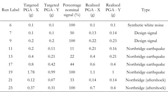
Table 2.1. Dimensions of mock-up structural elements ... 35

Table 2.2: Ground motions’ sequence considered in the blind prediction contest ... 36

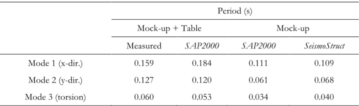
Table 2.3. Comparison between the periods of vibration measured in the experimental test and

computed with different numerical models ... 40

Table 2.4: Relative error associated with the accelerations and displacements measured along X

and Y directions during RUN 19 ... 44

Table 3.1. Modal properties of Structure 1 ... 48

Table 3.2. Structures 2 and 3: Section and material details ... 51

Table 3.3. Modal properties of Structure 2 ... 52

Table 3.4. Estimations of plastic hinge length for the different structures ... 55

Table 3.5. Element discretization scheme adopted for the different structures ... 56

Table 3.6. Sensitivity parameters considered in the parametric study ... 58

Table 3.7. Elastic vibration periods of Structure 2 for different SP modelling options ... 71

Table 5.1. List of input parameters for the proposed bond-slip numerical model ... 131

Table 5.2. Parameters defining the bond-slip relation for deformed ... 134

Table 5.3. Parameters defining the bond-slip relation for deformed rebars under expected

splitting failure (adapted from fib [2011]) ... 136

Table 5.4. Parameters defining the bond-slip relation for plain rebars (adapted from fib [2011]) . 138

Table 5.5. Properties considered for the comparative study ... 158

Table 5.6. IP spacing and corresponding number of IPs ... 158

Table 6.1. Mechanical and material properties of the Test 19 specimen, as well as numerical

parameters adopted for the reference model ... 182

Table 6.2. Parameters and properties considered in the sensitivity analysis ... 184

Table 6.3. Experimental properties and numerical parameters adopted for test SD30, SD50 and

SD70, performed by Shima et al. [1987b] ... 201

Table 6.4. Experimental properties and numerical parameters adopted for tests P.16.16.2 and

(26)

Table 6.5. Experimental properties and numerical parameters adopted for Test 9 and Test 19 specimens ... 209

Table 6.6. Material properties adopted to model the RC frame ... 224

Table 6.7. Cross-sectional properties of the different members of the PRTD RC frame ... 225

Table 6.8. Bond-slip parameters adopted for the PRTD RC frame ... 230

Table 6.9. Comparison between experimental and numerical periods of vibration of the RC

(27)

LIST OF SYMBOLS

a1, a2 = Rayleigh Proportionality Parameters

c = Damping Coefficient

db = Diameter of Longitudinal Rebar

f = Frequency of Vibration fc = Concrete Compressive Stress

fcm = Mean Concrete Compressive Stress

fctm = Mean Concrete Tensile Stress

fy = Yield Stress of Steel

fym = Mean Yield Stress of Steel

fu = Ultimate Stress of Steel

fum = Mean Ultimate Stress of Steel

fr = Bond Index

k = Stiffness m = Mass

r = Strain Hardening Parameter

s = Spacing Between Transvers Reinforcement

t = Time

u = Relative Displacement

𝑢 = Relative Velocity

𝑢 = Relative Acceleration

(28)

wcr = Crack width

A0 = Area of Monotonic Bond-Slip Curve

A1, A2 = Shape Parameters in Reinforcement Models

Ab = Area of Rebar

Ac = Area of Concrete Fibre

Acyc = Cumulative Area of Cyclic Hysteresis

As = Shear Area

Cclear = Clear Spacing Between Rebar Ribs

Dhook = Diameter of Hook

Ec = Modulus of Elasticity of Concrete

Es = Modulus of Elasticity of Steel

Es,p = Modulus of Elasticity at Strain Hardening

Fbar = Rebar Force

Fbond = Bond Force

Fc = Concrete Fibre Force

Ffibre = Fibre Force

F0 = Force at Loaded-End of Rebar

F0,trial = Trial Force at Loaded-End of Rebar

G = Shear Modulus

I = Moment of Inertia

IP = Integration Point

IPeq = Integration Point of Equilibrium

Kfibre = Fibre Stiffness

KIP = Integration Point Stiffness

Ks = Shear Stiffness

(29)

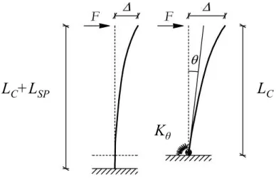
KΘ = Rotational Stiffness

Kunl/rel = Unload and Reload Bond-Slip Stiffness

LC = Shear Span

Ld = Development Length

Le = Embedment Length

Leq = Equivalent Embedment Length

Li = Influence Length

LIP = Distance Between Integration Points

LP = Plastic Hinge Length

Ls = Straight Embedment Length

LSP = Strain Penetration Length

M = Bending Moment

N = Axial Force

Pb = Perimeter of Rebar

Ptr = Transverse Pressure

Rr = Relative Rib Area

S = Rebar Slip

S0 = Slip at Loaded-End of Rebar

SLe = Slip at Free-End of Rebar

SR = Rib Spacing

T = Period of Vibration

α = Bond Stress Parameter

εs = Steel Strain

εs0 = Steel Strain at Loaded-End of Rebar

εs,y = Yield Steel Strain

(30)

εc = Strain at Peak Concrete Stress

µ = Ductility

ξ = Critical Damping Ratio

π = Pi

ρl = Longitudinal Reinforcement Ratio

ρv = Transverse Reinforcement Ratio

σ = Stress

σc = Concrete Stress

τ = Bond Stress

τi = Generic Bond Stress

τm = Modified Bond Stress

τmax = Maximum Bond Stress

τf = Friction Bond Stress

ω = Angular Frequency of Vibration

Δ = Displacement

Δt = Time-Step

Θ = Rotation

Ø = Rebar Diameter / Curvature

Øy = Yield Curvature

Ωcr = Longitudinal Cracking Bond Factor

Ωcyc = CyclicDegradation Bond Factor

Ωp.tr = Transverse Pressure Bond Factor

(31)

1. INTRODUCTION

1.1 RESEARCH MOTIVATION AND OBJECTIVES

Since the appearance of simplified methodologies in the mid-20th_{century (e.g. [Muto,}

1956]), the seismic analysis of structures witnessed a great evolution up to the present days. Modern seismic design and assessment of structures tends to rely heavily on numerical simulation tools. Their development has accompanied the exponential growth of computational power, the advancement of solution algorithms, and the increasing availability of experimental data for model calibration.

Among the available methodologies, nonlinear dynamic analysis appears as the most advanced simulation tool since it allows for an explicit simulation of the structural response to an actual ground motion. Past blind prediction tests showed that, by making use of specific combinations of modelling options, the nonlinear dynamic response of reinforced concrete (RC) structures can be predicted with satisfactory accuracy. Figure 1.1 presents a summarised comparison between the experimentally measured maximum displacements and the numerical estimates submitted by the author and supervisors to two different international blind prediction challenges [Terzic et al., 2015; Costa et al., 2012]. Although the authors won the competition for Structures 2 and 3 (among 38 international teams), and obtained an ’Award of Excellence‘ for Structure 1 (among 41 international teams), it can be observed that there is ample space for simulation improvements.

Figure 1.1. Comparison between experimental results and numerical simulations submitted by the authors to different blind prediction challenges: maximum displacements for seismic motions of increasing intensity

1 2 3 4 5 6 −300 −200 −100 0 100 200 300 400 500 600 Eqk Number Max. Displacement (mm) Structure 1 Numerical Experimental 1 2 3 4 −150 −100 −50 0 50 100 150 Eqk Number Max. Displacement (mm) Structure 2 Numerical Experimental 1 2 3 4 −80 −60 −40 −20 0 20 40 60 80 100 Eqk Number Max. Displacement (mm) Structure 3 Numerical Experimental

(32)

The comparison of other physically measurable quantities at a more local level would further emphasize this preliminary observation. The abovementioned structures, which will be used throughout the present work, are described along with their corresponding experimental program in Section 3.1.

Furthermore, the preceding blind challenges have also evidenced a significant dispersion of predictions between the participating teams, which is more meaningful upon observation that such scatter takes place also between teams using the same structural simulation software as the winning team. This clear symptom of lack of consensual modelling principles causes concern and makes it fundamental to identify the main sources of inaccuracy in nonlinear structural analysis so as to progressively reach an agreement on the modelling options that minimize the gap between experimental and numerical response.

Figure 1.2, which shows the results achieved by all the participants on the blind prediction pier test corresponding to Structure 1 [Terzic et al., 2015; Schoettler et al., 2015], further supports the comments above. It is noted that, even for such a rather simple structure (a single pier with a mass at the top), the predictions for the response parameters submitted by the different teams vary by more than one order of magnitude.

Figure 1.2. Comparison between experimental results and numerical simulations on the ‘Concrete Column Blind Prediction Contest 2010’: maximum horizontal displacement (left) and maximum bending moment (right) (adapted from Terzic et al. [2015])

(33)

A first and crucial decision that every engineer faces when modelling a frame structure for seismic analysis – which is further conditioned by the available structural analysis software – is related to the choice of the element type. Amongst the available approaches, frame models developed in the framework of the Euler-Bernoulli beam theory with distributed plasticity are often considered to offer the best compromise between the degree of output detail and computational demand, at least for research or specialized earthquake engineering applications. Lumped plasticity models are simpler and computationally lighter, but they do not allow modelling the spread of inelasticity throughout the member. In addition, the use of such approach requires the a priori knowledge of the location and extension of inelasticity, which is only possible under certain limiting assumptions [Hines et al., 2004]. Moreover, modelling elements through lumped plasticity models requires a high level of expertise in order to define appropriate constitutive hysteretic relations taking into account the variations of axial force. Hereinafter, the present work focuses solely on distributed plasticity models.

Recent attempts have been made to identify and measure the importance of different modelling options (e.g., [Sousa et al., 2012; Blandon, 2012; Yazgan and Dazio, 2011a, 2011b]). The current study intends to consolidate some of these findings and to further extend them in order to progressively bridge the gap between solidly established theoretical principles and experimental results from shake table tests. Based on the conclusions of previous studies and preliminary tests by the authors, it was found particularly pertinent to analyse the following modelling options given their potential to more critically affect the finite element simulation results and therefore the prediction of engineering demand parameters (EDPs) on which performance-based assessment is ultimately based:

1. Equivalent viscous damping models

2. Element formulation and discretization scheme 3. Strain penetration effects

4. Material constitutive models

5. Numerical integration and time-step size

These variables were used in the numerical applications presented in Chapter 3, wherein the shake table responses of the three foregoing RC structures served as a benchmark. The goodness-of-fit of each approach, assessed in terms of lateral displacements, as well as accelerations when available, is determined based on the error associated with the peak values measured during each time-history record, together with a new frequency-domain error capable of evaluating the records under comparison in terms of both amplitude and frequency content.

(34)

The sensitivity study carried out shows that some of the modelling options seem to present a matured level of development and implementation, namely regarding the material constitutive models as well as the domain integration algorithms and time-step size. However, important limitations were identified in other modelling options, namely with respect to the use of equivalent viscous damping models, alternative discretization schemes and the simulation of strain penetration effects. In particular, the simplified modelling approaches that are typically used to model the latter in common nonlinear software packages appear to be highly unsatisfactory.

When subjected to seismic loading, RC members often depict localized member-end deformations due to rebar slippage between adjacent members, such as beam-column and column-footing joints. Past experimental programs (e.g., [Sezen and Moehle, 2004] and [Goodnight et al., 2015a]) indicate that the resultant member-end rotations can contribute up to 40% of the lateral deformation of the RC members (Figure 1.3).

Despite the recognized importance of strain penetration effects on the response of RC structures, the consideration of such effects in numerical models is still not widespread. The employment of advanced bond-slip models within detailed 3D finite element (FE) formulations, capable of simulating continuous domains with highly discretized meshes, has witnessed great advances over the recent years with encouraging results. Nonetheless, these modelling approaches are computationally heavy and, hence, inapplicable for most practical seismic analysis of RC framed structures.

Alternatively, the consideration of beam-column elements featuring lumped or distributed plasticity represents an alternative solution that is computationally more efficient and, therefore, preferable for most common engineering applications. Unfortunately, for such modelling approaches, the explicit simulation of the interface between the reinforcing bars and the surrounding concrete is not a straightforward task. Therefore, the inclusion of bond-slip effects in beam-column element models has been essentially achieved through the employment of simplified formulations based on empirical relations.

Figure 1.3. Contribution of different deformation mechanisms to the total lateral displacement according to Sezen and Moehle [2004]

Also shown in Figure 7 are the transverse reinforcement strain distributions over the height of columns. The strains were plotted in each loading direction at first yielding in the longitudinal bars, at peak lateral load, and at loss of lateral capacity (ultimate), which is assumed to occur when the lateral load drops to 80 percent of peak lateral strength is reached. At peak and ultimate levels, the transverse reinforcement strains tend to be the largest some short distance away from column ends, where most of

the damage and extensive cracking were observed due to combined high flexural and shear demand. As the damage progresses, more cracks intersect the transverse reinforcement and consequently increase the strains in the bars crossing the cracks. For instance, in Specimen-2 with less damage and less number of cracks at the onset of failure, the strains in the transverse direction were much smaller prior to failure.

Deformation components

As illustrated in Figure 8, total column lateral displacement measured at the top of each column can be assumed to be the summation of deformations due to: a) flexure, ∆flexure; b) longitudinal bar slip at column

ends, ∆slip; and c) shear, ∆shear. Experimental flexure, bar slip, and shear deformations are obtained and

presented in the following sections. Figure 9 shows the contribution of these deformation components to the total column lateral displacement at peak displacement during each displacement cycle. The results indicate that approximately 40 to 60 percent of total lateral displacement is due to flexure, while 25 to 40 percent is due to bar slip deformations. Typically the shear displacement component is relatively small especially in the elastic range and under very high axial loads. However, the contribution of shear deformations can increase significantly as in Specimen-1. In this column, the contribution of shear deformations grew gradually to about 20 percent of the total deformation at a displacement ductility of two, at which time shear strength degradation became severe and shear deformations increased dramatically to about 40 percent of total displacement.

∆_total / ∆_y percentage of displacement shear slip flexure Specimen−1 0 1 2 3 0 20 40 60 80 100 ∆_total / ∆_y Specimen−2 0 0.5 1 1.5 0 20 40 60 80 100 ∆_total / ∆_y Specimen−3 0 1 2 3 0 20 40 60 80 100 Specimen−4 ∆_total / ∆_y 0 1 2 3 0 20 40 60 80 100

Figure 9 Contribution of displacement components to total lateral displacement

(35)

The present study aims at overcoming the foregoing limitation through the development of an explicit bond-slip model applicable to general fibre-based beam-column elements. Adopting a state-of-the-art bond stress-slip cyclic constitutive model, it introduces a zero-length element to simulate the localized member-end deformations resulting from the contribution of the bond-slip response associated to each rebar of a given RC cross-section. Along with the material properties and anchorage conditions, the proposed nonlinear model also accounts for cyclic degradation and rebar yielding effects. Validation studies conducted with the proposed numerical formulation reveal a good agreement with past experimental tests, evidencing an encouraging numerical stability and accuracy at the expense of an acceptable additional computational effort.

1.2 THESIS OUTLINE

The present dissertation is organized in 7 chapters. Following the current introductory text (Chapter 1), Chapter 2 presents a brief discussion on the theoretical framework and current recommendations enveloping modelling options that, in the author’s opinion, represent some of the main sources of epistemic uncertainty in current nonlinear analysis of RC framed structures. In addition, this chapter also discusses the consideration of simplified wide-column models to simulate the response of RC wall buildings.

Based on the above findings, Chapter 3 presents a sensitivity study using three different RC structures featuring alternative modelling options. The analysis of the results allows extracting important indications on the appropriateness of the different solutions considered. Furthermore, this chapter puts into evidence the need to develop improved numerical models to simulate the strain penetration effects in RC members.

The subsequent three chapters, which constitute the core of the thesis, are dedicated to conceptualize, implement and validate a novel bond-slip model for fibre-based nonlinear beam-column elements. Namely, Chapter 4 provides a detailed state-of-the-art review on bond behaviour under different anchorage conditions, together with the identification and characterization of the most relevant numerical approaches currently available to model strain penetration effects.

Chapter 5 presents the theoretical background of the proposed bond-slip model alongside with the numerical formulation, solution algorithms and implementation strategies adopted. The adopted bond stress-slip constitutive relation is also described and validated.

Chapter 6 is divided in two parts. The first introduces a quantitative study on the relative importance of the different anchorage parameters incorporated in the proposed bond-slip model. The second validates the numerical response computed with the proposed model

(36)

against a wide selection of experimental tests, evaluating the response at different structural levels while considering progressively more complex structures and loading demands.

Finally, the main conclusions of the present research work are summarized in Chapter 7, while some suggestions for future developments are proposed.

(37)

2. NONLINEAR MODELLING OF RC STRUCTURES

Over the last years, attempts have been made to identify and measure the importance of different modelling options (e.g., [Sousa et al., 2012; Blandon, 2012; Yazgan and Dazio, 2011a, 2011b]). This work intends to consolidate some of these findings and further extend them in order to progressively bridge the gap between solidly established theoretical principles and shaking table tests’ results.

The present chapter presents a comprehensive theoretical discussion on the following sensitivity parameters:

• Equivalent viscous damping models

• Element formulation and discretization scheme • Strain penetration effects

• Material constitutive models

• Numerical integration algorithms and time-step size

In Chapter 3, the response of three different structures used in international blind prediction challenges will serve as benchmarks for a sensitivity study considering the above listed modelling options.

At the end of the present chapter, a discussion on the use of simplified wide-column models to simulate the response of RC wall buildings is carried out. The appropriateness of this simplified solution is appraised against a shake table test of a scaled U-shaped RC mockup representative of a component extracted from a nuclear power plant building.

2.1 DAMPING

“In spite of a large amount of research, understanding of damping mechanisms is quite primitive”. This excerpt extracted from Adhikari [2000] summarises the state-of-the-art regarding the comprehension of damping mechanisms and the corresponding simulation with current numerical tools, which are explored in more detail in the subsequent sections.

(38)

2.1.1 Damping in Structures

Damping in structures is generally associated with the decay of free-vibration motion due to energy dissipation mechanisms in structural, non-structural, and substructural components. In real structures, several irreversible thermodynamic processes concur to such decay, e.g., global damage in the components, internal friction between materials or at connections, opening and closing of micro-cracks in the materials, and friction between the structure itself and non-structural elements [Chopra, 1995].

Measuring and comparing damping of different structures subjected to distinct loadings is a favoured way to understand the energy dissipation mechanisms in structures. The relation between damping values and structural period of vibration has been recognized for a long time [Wakabayashi, 1986]. In Section 2.4.3.4. of the report PEER/ATC 72-1 [PEER/ATC, 2010], a summary of damping ratios inferred from decrements in peak-to-peak response in free vibrations following shake table or pull-release tests shows that the modal damping values measured in undamaged RC frame (or frame-wall) structures and steel braced frame systems ranged from about 0.5% to 3.5% of critical.

Not surprisingly, significantly damaged structures exhibit modal damping ratios that can go up to 11% [PEER/ATC, 2010]. The compilation of such results indicates that the classical assumption of 5% of critical damping, traditionally adopted in the not-so-distant past as a reference modal damping ratio for RC buildings, may result in a non-negligible overestimation of the energy dissipated during elastic dynamic response.

In order to better understand the energy dissipation associated with different structures, the following sections summarise the results of several studies dedicated to quantify and correlate damping values with distinct structural properties. This information is relevant in the sense that it can provide indications on the amount and type of damping that one can define in nonlinear dynamic analysis.

It should be noted that damping measurements can be influenced by the use of different system identification procedures and quality of the data series considered [Brownjohn and Carden, 2007]. Despite the potential dispersion resulting from this issue, the following observations indicate important trends on what respects the quantification and variation of damping in buildings.

(39)

It is commonly accepted that damage, and consequently energy dissipation, increases with the amplitude to which the structures are subjected. Based on a significant full-scale measurement database, Jeary [1986] proposed a model that relates the damping in buildings with the amplitude of their deformations (Figure 2.1).

Figure 2.1. Variation of damping with amplitude [Fang et al., 1999]

According to this model, at very low amplitudes only the large-scale imperfections are mobilized (e.g. interface of structural elements), whilst for increasing amplitudes the largest material imperfections start to be mobilized. Eventually, all possible mechanisms are activated and even for increasing amplitude, the energy dissipation remains constant [Jeary, 1997].

Over the last two decades, a number of authors proposed predictive expressions for modal damping ratios based on data measured from hundreds of existing buildings. The results presented in Figure 2.2 provides a comparison between the prediction models proposed by Lagomarsino [1993] and Satake et al. [2003] against a large database comprising measurements on 205 buildings in Japan.

Fig. 1. Generalized damping characteristic.

damping (!_{!) and (2) a rate of increase of damping with amplitude (}!_{"). This approach}

leads to the conclusion that absolute value of damping !_!at amplitude x_{" can be} estimated by the following expression:

!_!"!_!#!_"[x"]

H (1)

where H is the height of the building.

It is well known that the damping of a building reflects the capacity of a structure to dissipate the kinetic energy of vibration. Wyatt [3] proposed that all significant energy losses are assumed to be caused by friction. Jeary [2] investigated the mechanism for the amplitude-dependent damping in buildings. Unlike the mass and the stiﬀness characteristics of a structural system, damping does not relate to a unique physical phenomenon. Several researchers investigated the sources of damping in buildings [2,4] and concluded that they comprise

(a) intrinsic internal material damping;

(b) structural damping due to the friction among the structural members; (c) foundation damping both due to radiation of energy and due to the structure and architectural finishes;

(d) aerodynamic damping due to the fanning action of the building in strong wind; (e) additional damping systems built into the structure.