Why standard risk models failed in the subprime crisis? An approach based on Extreme Value Theory as a measure to quantify market risk of equity securities and portfolios

WHY STANDARD RISK MODELS FAILED IN THE SUBPRIME

CRISIS?

An approach based on Extreme Value Theory as a measure to quantify

market risk of equity securities and portfolios

Áurea Ponte Marques

Dissertação submetida como requisito parcial para obtenção do grau

de Mestre em Finanças

Orientador:

Professor Doutor Mohamed Azzim Gulamhussen, Prof. Auxiliar, ISCTE Business School, Departamento de Finanças

The assessment of risk is an important and complex task with which market regulators and financial institutions are faced, especially after the last subprime crisis. It is argued that since market data is endogenous to market behaviour, statistical analysis made in times of stability does not provide much guidance in times of crisis. It is well known that the use of Gaussian models to assess financial risk leads to an underestimation of risk. The reason is because these models are unable to capture some important facts such as heavy tails which indicate the presence of large fluctuations in returns.

This thesis provides an overview of the role of extreme value theory in risk management, as a method for modelling and measuring extreme risks. In this empirical study, the performance of different models in estimating value at risk and expected tail loss, using historical data, are compared. Daily returns of nine popular indices (PSI20, CAC40, DAX, Nikkei225, FTSE100, S&P500, Nasdaq, Dow Jones and Sensex) and seven stock market firms (Apple, Microsoft, Lehman Brothers, BES, BCP, General Electric and Goldman Sachs), during the period from 1999 to 2009, are modelled with empirical (or historical), Gaussian and generalized Pareto (peaks over threshold technique of extreme value theory). It is shown that the generalized Pareto distribution fits well to the extreme values using pre-crisis data. The results support the assumption of fat-tailed distributions of asset returns. As expected, the backtesting results show that extreme value theory, in both value at risk and expected tail loss estimation, outperform other models with normality assumption in all tests. Additionally, the results of the generalized Pareto distribution model are not significantly different from the empirical model. Further topics of interest, including software for extreme value theory to compute a tail risk measure, such as Matlab, are also presented.

Keywords: Value at risk, Expected Tail Loss, Extreme Value Theory, Generalized Pareto

Distribution, Basel II

iv I would like to thank my supervisor, Professor Mohamed Azzim Gulamhussen. Thanks are also due to my professional colleagues at Banco de Portugal Fernando Infante, João Mineiro, José Rosas, Pedro Nunes and Teresa Urbano for their friendship and useful comments.

Abstract ... iii Acknowledgement ... iv Contents ... v 1. Introduction ... 1 2. Literature review ... 6 3. Theoretical Framework ... 11

3.1. Value at Risk (VaR) ... 11

3.2. Coherent risk measures and Expected Tail Loss (ETL) ... 12

3.3. Extreme Value Theory ... 14

4. Empirical study ... 18

4.1. Data and methods ... 19

4.2. Empirical tests and estimated parameters ... 20

4.3. Empirical tests and results ... 25

5. Conclusions ... 29

References ... 33

Tables ... 43

Figures ... 49

vi Apple Apple Inc.

ARCH Autoregressive Conditional Heteroskedasticity BCP Banco Comercial Português, S.A.

BES Banco Espírito Santo, S.A.

BIS Bank for International Settlements

CAC40 Cotation Assistée en Continu - French stock index Committee Basel Committee on Banking Supervision

CVAR Conditional Value at Risk (the same meaning as ETL) DAX Deutscher Aktien Index - German stock index

DJ Dow Jones Industrial Average - American stock index ES Expected Shortfall (the same meaning as ETL)

ETL Expected Tail Loss EVT Extreme Value Theory

EWMA Exponentially Weighted Moving Average

FTSE100 Financial Times Stock Exchange - English stock index GARCH Generalized Autoregressive Conditional Heteroskedasticity GE General Electric Company

GED Generalized Error Distribution GEV Generalized Extreme Value GPD Generalized Pareto Distribution GS The Goldman Sachs Group, Inc. HS Historical Simulation

I.i.d Independent and Identically Distributed LB Lehman Brothers Holdings Inc.

LEL-RM Limited Expected Losses based Risk Management LR Likelihood ratio statistics

LRuc Likelihood ratio statistics of The Unconditional Coverage Test MS Microsoft Corporation

Nasdaq National Association of Securities Dealers Automated Quotations - American stock index

Nikkei225 Nihon Keizai Shimbun - Japanese stock index POT Peaks Over Threshold

PSI20 Portuguese Stock Índex P&L Profits and Losses QQ-plot Quantile-Quantile plot

Sensex Bombay Stock Exchange Sensitive Index - Indian stock market index S&P500 Standard & Poors - American stock index

USA United States of America VaR Value at Risk

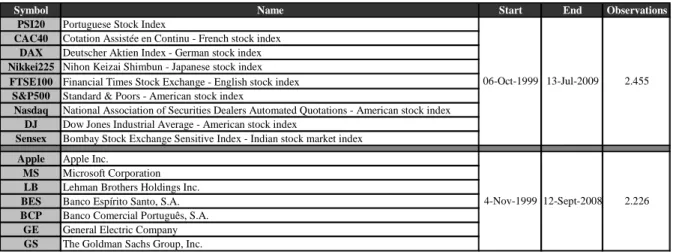
Table I – Data analyzed ... 43

Tables II - Basic statistics ... 43

Tables III - Covariance Matrix ... 44

Tables IV - Correlation matrix ... 44

Table V – Descriptive statistics of daily returns for nine indices and seven stock market firms ... 45

Tables VI - Descriptive assessment of empirical, normal and GPD models in VaR and ETL estimation ... 46

Tables VII - Supervisory Framework for the use of “backtesting” in conjunction with the internal models approach to market risk capital requirements ... 47

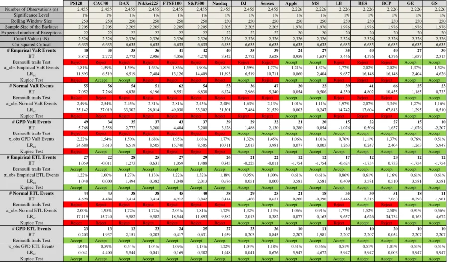
Table VIII - Descriptive statistics of “backtesting” the six models of VaR and ETL estimation by Bernoulli test and Kupiec test ... 48

viii

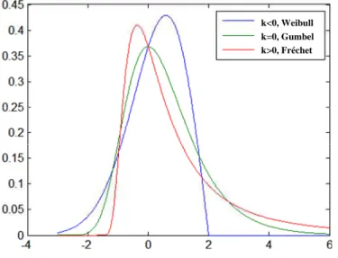
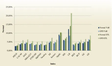
Figure I - Three possible limiting extreme value distributions for the standardized maxima ... 49 Figures II – The historical prices and index returns series ... 50 Figures III – Returns and respective histogram for the nine index portfolio (seven countries) and for the seven firms stock market portfolio ... 58 Figures IV - Histograms for the nine index portfolio (seven countries) and for the seven firms stock market portfolio (VaR and ETL estimation) ... 59 Figures V – Backtesting representation of VaR and ETL estimation for the nine index portfolio (seven countries) and for the seven firms stock market portfolio (VaR and ETL estimation) ... 60 Figures VI – Risk and return representation of the nine index portfolio (seven countries) and the seven firms stock market portfolio ... 61 Figures VII – Visual comparison between empirical, normal and GPD models in VaR and ETL

estimations ... 62 Figure VIII - Visual comparison between normal and GPD models in VaR and ETL estimations ... 63 Figures IX - Checking the asymptotic normality assumption: Histograms of the bootstrap replicates 64 Figures X - Checking the asymptotic normality assumption: QQ plot ... 67 Figures XI - Illustration of the result before filter the returns for each price and index using GARCH method (without i.i.d. assumption) – Example Lehman Brothers ... 70 Figures XII – Illustration of the result after filter the returns for each price and index using GARCH method (i.i.d. assumption) – Example Lehman Brothers ... 71 Figures XIII – Estimation of the semi-parametric cumulative distribution function – Example Lehman Brothers ... 72 Figures XIV - Checking the Fit Visually ... 73

Matlab Code I - Prices and Returns ... 76

Matlab Code II - Filter the Returns for Each Price (GARCH) ... 77

Matlab Code III - Estimate the Semi-Parametric Cumulative Distributions Functions ... 78

Matlab Code IV - Estimating parameters ... 79

Matlab Code V - Assess the GPD Fit ... 79

Matlab Code VI - Computing Standard Errors for the Parameter Estimates ... 79

Matlab Code VII - Checking the Asymptotic Normality Assumption ... 80

Excel Macros Code IX - Mean Exceedances ... 81

1

1. Introduction

In recent years value at risk (VaR) has become a very popular measure of market risk and it has been adopted by central bank regulators as the major determinant of the capital requirements for banks in order to cover for potential losses arising from the market risks they are bearing. Recent directives issued by the Basel Committee have established VaR as the standard measure to quantify market risk. The solvency of banks is mainly important for the stability of the financial system. Central banks and the Basel Committee have a well-built concern in systemic risk, where insolvency in one sector of an economy can lead to a national crisis. The global recession following the stock market crash of 1987 prompted a revision of banking regulations as well as new minimum requirements owned by banks that were imposed in the G10 countries, and after adopted by the most of the countries in the world.

According to Jorion (2007), unforeseen adverse situations unaccounted for by existing models triggered huge losses, eventually ending in bankruptcies or almost bankruptcies1. The financial crisis that started in August 2007 is a case study for extreme risks and risk management practices. In recent years, the problem of extreme risks in financial markets has become topical following the crises in the Asian and Russian markets, and the unexpected big losses of investment banks such as Barings and Daiwa. The events prompted regulators to address the issue, and from the advent of the Basel Capital Accord of 19962 there has been a strong concern about quantifying market risk because banks were demanded to put up risk-adjusted capital as a buffer against likely shortfalls. The Amendment to the Basel Accord in 19963

and the broad lines maintained in the Basel Capital Accord of 20044 allowed financial institutions to employ their own internal market risk management models in order to determine capital requirements.

Unlike economic capital, when estimating the legal minimum required for the banks against its market risk exposures, the manager can use several risk models and risk metrics or simply apply the standardized rules that are set by the regulators. The banks can use an advanced risk model to estimate the market risk, validated by the regulator and provided that the risk management structure in the bank satisfies certain qualitative criteria. It can be one of the two broad types, either a scenario model or a VaR model. The scenario model is used by

1_{The last remarkable cases are Northern Rock, Bear Stearns, ANB Financial, First Integrity Bank, Roskilde}

Bank, IndyMac, First Heritage Bank, First National Bank of Nevada, IKB, Silver State, Fannie Mae, Freddie Mac, Lehman Brothers, AIG and Washington Mutual.

2 _{See http://www.bis.org/publ/bcbs04a.pdf .} 3 _{See http://www.bis.org/publ/bcbs24a.pdf .} 4

smaller banks based on an aggregate maximum loss whereas major banks usually adopt the VaR model.

Since the financial crisis began in mid-2007, an important source of losses and the build up of leverage occurred in the trading book. A main contributing factor was that the current capital framework for market risk, based on the 1996 Amendment to the Capital Accord to incorporate market risks, does not capture some key risks. In response, the Basel Committee on Banking Supervision (the Committee) supplements the current VaR based trading book framework with an incremental risk capital charge, which includes default risk as well as migration risk, for unsecuritised credit products. An additional response to the crisis is the introduction of a “stressed VaR” requirement. Losses in most banks trading books during the financial crisis have been significantly higher than the minimum capital requirements under the former Pillar 1 market risk rules.

In June 2006, the Committee published a comprehensive version of the Basel II framework5 which included the June 2004 Basel II framework, the elements of the 1988 Accord that were not revised during the Basel II process, the 1996 amendment to the Capital Accord to incorporate market risks and the July 2005 paper on the application of Basel II to trading activities and the treatment of double default effects. The Committee released consultative documents on the revisions to the Basel II market risk framework and the guidelines for computing capital for incremental risk in the trading book in July 20086 and more recently in July 20097. The Committee has decided that the incremental risk capital charge should capture not only default risk but also migration risk. This decision is reflected in the proposed revisions to the Basel II market risk framework. Additional guidance on the incremental risk capital charge is provided in a separate document, the guidelines for computing capital for incremental risk in the trading book (referred to as “the Guidelines”)8.

According to the revised Basel II market risk framework, the precise number and composition of the stress scenarios to be applied will be determined by the Committee in consultation with the industry by March 2010. Furthermore, the Committee will evaluate a floor for the comprehensive risk capital charge which could be expressed as a percentage of the charge applicable under the standardised measurement method. This evaluation will be based on a quantitative impact study to be conducted in 2010. The improvements in the Basel II framework concerning internal VaR models in particular require banks to justify any

5 _{See http://www.bis.org/publ/bcbs128.pdf .} 6 _{See http://www.bis.org/publ/bcbs140.pdf .} 7 _{See http://www.bis.org/publ/bcbs158.pdf .} 8 See http://www.bis.org/publ/bcbs159.pdf .

3 factors used in pricing which are left out in the calculation of VaR. They will also be required to use hypothetical backtesting at least for validation, to update market data at least monthly. To complement the incremental risk capital framework, the Committee extends the scope of the prudent valuation guidance to all positions subject to fair value accounting and make the language more consistent with the existing accounting guidance. The Committee has already conducted a preliminary analysis of the impact of an incremental risk capital charge where it included merely the default and migration risks, largely relying on the data collected from its quantitative impact study on incremental default risk in late 2007. It has collected additional data in 2009 to assess the impact of changes to the trading book capital framework. In the coming months, the Committee will review the calibration of the market risk framework in light of the results of this impact assessment. This review will include multipliers to the current and “stressed VaR” numbers. Banks are expected to comply with the revised requirements by December 31, 2010.

Under the revisions of the Basel II market risk framework proposed by the Basel Committee on Banking Supervision, VaR must be computed on a daily basis in a 99th percentile. In calculating VaR, an instantaneous price shock equivalent to a ten-day movement in prices is to be used, i.e., the minimum “holding period” will be ten trading days. The choice of historical observation period (sample period) for calculating VaR will be constrained to a minimum length of one year. Banks must update their data sets frequently by no less than once every month and reassess them whenever market prices are subject to material changes. No particular type of model is prescribed in the framework, however each model used need to capture all the material risks run by the bank. In this way, banks can use models based, for example, on variance-covariance matrices, historical simulations or Monte Carlo simulations. Banks can also recognise empirical correlations within broad risk categories (e.g. interest rates, exchange rates, equity prices and commodity prices, including related options volatilities in each risk factor category). In addition, banks must calculate the above mentioned “stressed VaR” measure. This measure is intended to replicate a VaR estimation that would be generated on the banks current portfolio if the relevant market factors were experiencing a period of stress and should therefore be based in the same conceptions than VaR, but with different calculations. Banks for International Settlements (BIS) did not prescribe any model to calculate this “stressed VaR” and banks can develop different techniques to translate this new addition9. The additional “stressed VaR”

9 _{BIS gives an example, for many portfolios, a 12-month period relating to significant losses in 2007/2008 would}

requirement will also help to reduce the procyclicality of the minimum capital requirements for market risk.

VaR is formally defined as a quantile of the forecasted distribution of profits and losses (P&L) over a time span. The practical advantages of VaR methodology are largely counterbalanced by theoretical flaws10 (see e.g. McNeil, Frey and Embrechts, 2005; Szegö, 2002 for a detailed review of VaR pitfalls), but, even so, VaR has become a regulatory exigency obliging financial institutions to obtain accurate and robust estimates in order to construct adequate capital structures.

The last years have been characterized by significant instabilities in the financial markets. With the latest market adversity started in the United States of America (USA) with the sub-prime mortgage crisis it is clear that there is a need for an approach that comes to terms with problems posed by extreme event estimation. Advances that have been made in VaR should not be lost with the probable (and well deserved) adoption of coherent risk measures into regulatory framework. This has led to numerous criticisms about the existing risk management systems and motivated the search for more appropriate methodologies able to cope with rare events that have heavy consequences. Concerning the extensive range of applications like risk management or regulatory requirements and considering that institutions can use their own approaches, the development of accurate techniques has become a topic of prime importance. While most methodologies could achieve that purpose for common everyday movements, they find themselves unable to account for unexpected events that take place in the crisis. It is well known that the use of Gaussian models to assess financial risk leads to an underestimation of risk. The reason is because these models are unable to capture some important facts such as heavy tails and volatility clustering which indicate the presence of large fluctuations in returns. By comparing the VaR and the Expected Tail Loss (ETL) calculated analytically and using simulations, but both approaches lead to almost the same result. Superior quality of VaR techniques can be employed to yield superior ETL forecasts. Academics and practitioners have extensively studied VaR to propose an unique risk management technique that generates accurate VaR estimations for long and short trading positions and for all types of financial assets. However, they have not yet succeeded as the testing frameworks of the proposals are still being developed. Numerous conditional volatility models that capture the main characteristics of asset returns (asymmetric and leptokurtic unconditional distribution of returns, power transformation and fractional integration of the

10

5 conditional variance) under four distributional assumptions (normal, generalized error distribution (GED), Student-t, and skewed Student-t) have been estimated to find the best model for financial markets, long and short trading positions, and two confidence levels. By following this procedure, the risk manager can significantly reduce the number of competing models that accurately predict both the VaR and the ETL measures. ETL estimations can be significantly improved by using the knowledge obtained from advances in VaR estimation. This way, the VaR and the ETL should be regarded as partners, not rivals.

Further than traditional approaches, various alternative distributions have been proposed to describe fat-tail characteristics. One of the most popularity is based on the Extreme Value Theory (EVT). EVT has traditionally been used in fields like civil engineering, hydrology, meteorology and actuarial applications concerning loss severity distributions, recently being devoted to financial purposes. EVT provides a framework in which an estimate of anticipated forces could be made using historical data. Today, EVT is used in telecommunications, ocean wave modelling, thermodynamics of earthquakes, memory cell failure and many other fields. It is important to be aware of the limitations implied by the adoption of the EVT paradigm. EVT models are developed using asymptotic arguments, which should be kept in mind when applying them to finite samples. This extreme model provides a method to estimate VaR at high quantiles of the distribution, consequently focusing on extraordinary and unusual circumstances. This method focuses on the tails behaviour of distribution of returns. Instead of forcing a single distribution for the entire sample, it investigates only the tails of the return distributions, given that only tails are important for extreme values. Backtesting EVT representations found that EVT schemes could help financial institutions to avoid huge losses arising from market fluctuations. This simple exercise illustrates the advantages of EVT.

The empirical study examines the dynamics of extreme values of overnight returns before and during a financial crisis. It is shown that the generalized Pareto distribution (GPD) using the EVT fits well to extreme values of the exceedances distribution. The examination of tails (extreme values) provides answers to the extreme movements expected in financial markets and in assessing the financial fragility. In order to accomplish this task, a series of computational tools have been selected, such as Statistics Toolbox and Optimization Toolbox, an integrated environment for risk assessment developed in Matlab R2009a. This standard numerical or statistical software now provide functions or routines that can be used for EVT applications. Matlab has been designated because it provides a well-suited programming

environment, where both numerical and interface design challenges can be met with a reduced development effort.

This thesis is structured as follows. In Section 2, the literature survey presents the definitions and reviews used in the empirical study. Section 3 delineates topics regarding the theoretical framework. Section 4 presents the empirical study that assesses the normal, the historical and the extreme values in risk management throughout the estimation of VaR and ETL. The empirical application is based on daily closings of the nine major developed market indices and seven stock market companies from, respectively, October 6, 1999 to July 13, 2009 and November 4, 1999 to September 12, 2008. In particular, the EVT results are used to model the distributions underlying the risk measures by computing the estimations of the tail risk parameters. Section 5 states the concluding remarks and outlines some directions for further research.

2. Literature review

Baumol (1963) made the first attempt to estimate the risk that financial institutions face when he proposed a measure based on a standard deviation adjusted to a confidence level parameter that reflects the attitude towards risk. Since JP Morgan made available its RiskMetrics system on the Internet in 1994, the popularity of VaR and with it the debate among researchers about the validity of the underlying statistical assumptions increased. This is because VaR is essentially a point estimate of the tails of the empirical distribution. The assumed distribution for each market variable in Hull and White (1998) can be chosen in a variety of ways. One possibility is to select an appropriate standard distribution (e.g. a mixture of normals) and use maximum likelihood methods to find the best fit parameters. Another possibility is to smooth the historical distribution (e.g. using a kernel estimator). Using high frequency data others “stylized facts” of real-life returns have been studied namely: volatility clustering, long range dependence and aggregational Gaussianity. Many econometric models have been suggested to explain part of these asset return behavior and among then this study uses the Generalized autoregressive conditionally heteroscedastic model (GARCH). Other models have been suggested to capture this behaviour (Rydberg, 2000). The Hull and White approach provides one way of bridging the gap between the model building and historical simulation approaches. It shows how the model building approach can be modified to incorporate some of the attractive features of the historical simulation approach. Angelidis and Degiannakis (2005) suggest that “(...) a risk manager must employ

7

trading positions (...)”, whereas Angelidis et al. (2004) considered that “(...) the ARCH structure that produces the most accurate VaR forecasts is different for every portfolio (...)”.

Furthermore, Guermat and Harris (2002) applied an exponentially weighted likelihood model in three equity portfolios (US, UK, and Japan) and proved its superiority to the GARCH model under the normal and the Student-t distributions in terms of two backtesting measures (unconditional and conditional coverage). Moreover, Angelidis and Degiannakis (2004) studied the forecasting performance of various risk models to estimate the one-day-ahead realized volatility and the daily VaR. Regarding only on the VaR forecasts, they support that it was more important to model the fat tailed underlying distribution than the fractional integration of the volatility process. Similarly, Bams et al. (2005) argued that complex (simple) tail models often lead to overestimation (underestimation) of the VaR. On the one hand, Taleb (1997) and Hoppe (1999) argued that the underlying statistical assumptions are violated because they could not capture many features of the financial markets (e.g. intelligent agents). Under the same framework, many researchers (see for example Beder, 1995 and Angelidis et al. (2004)) showed that different risk management techniques produced different VaR forecasts and therefore, these risk estimates might be imprecise.

Bams and Wielhouwer (2000) drew similar conclusions, although sophisticated tail modelling results in better VaR estimates but with more uncertainty. They concluded that if the data generating process is close to be integrated, the use of the more general GARCH model introduces estimation error, which might result in the superiority of Exponentially Weighted Moving Average (EWMA). Guermat and Harris (2002) found that EWMA-based VaR forecasts are excessively volatile and unnecessarily high, when returns do not have conditionally normal distribution but fat tails. According to Brooks and Persand (2003) relative performance of different models depends on the loss function used but GARCH models provide reasonably accurate VaR. Christoffersen, Hahn and Inoue (2001) demonstrated that different models (EWMA, GARCH, Implied Volatility) might be optimal for different probability levels. Berkowitz and O'Brien (2002) examined VaR models used by six leading US banks. Their results indicated that these models are in some cases highly inaccurate. Their results indicated that banks models have difficulty dealing with changes in volatility. Žiković (2007) found that widespread VaR model consistently underpredict the true levels of risk especially at higher confidence intervals and that semi-parametric models provide superior VaR forecasts in transitional economies.

The normal or Gaussian model is well accepted in Economics and Finance because of the central limit theorem and the simplicity of concepts. The portfolio selection method of

Markowitz (1952), Sharpe’s (1964) market equilibrium model and Black and Scholes (1973) option pricing theory are examples of developments taking a parent normal model as granted. This state of the art collapsed with the widespread use of computers, which provided exuberant evidence that skewness and kurtosis of empirical data could not support a normal fit in many instances of modelling financial returns. The standard VaR measure presumes that asset returns are normally distributed, whereas it is widely documented that they really exhibit non-zero skewness and excess kurtosis and, hence, the VaR measure either underestimates or overestimates the true risk. On the other hand, even if VaR is useful for financial institutions to understand the risk they face, it is now widely believed that VaR is not the best risk measure.

Although VaR is useful for financial institutions to see the contours of the risks they face, a growing number of papers clearly show that VaR is not an adequate risk measure. As a result, more general complex measures of risk have been proposed. VaR suffers from various shortcomings pointed out in recent studies. For example, numerical instability and difficulties occur for non-normal loss distributions, especially in the presence of “fat tails” or/and empirical discreteness. Artzner et al. (1997, 1998 and 1999) used an axiomatic approach to the problem of defining a satisfactory risk measure. Their study defined attributes that any good risk measure should satisfy and called for risk measures that satisfy these axioms “coherent”. Additionally, the study demonstrate that VaR is not necessarily sub-additive, i.e., the VaR of a portfolio may be greater than the sum of individual VaR and therefore, managing risk by using it may fail to automatically stimulate diversification. VaR can only be made sub-additive if an usually implausible assumption is imposed on returns being normally (or more generally, elliptically) distributed. Sub-additivity expresses the fact that a portfolio will risk an amount, which is at most the sum of the separate amounts risked by its sub-portfolios. Moreover, it does not indicate the size of the potential loss, given that this loss exceeds the VaR. Furthermore, VaR is not a coherent measure of risk in the sense of Delbaen (2002) and Arztner et al. (1997, 1998 and 1999), and it does not take into account the severity of an incurred adverse loss event. A simple alternative measure of risk with some significant advantages over VaR is conditional VaR, expected shortfall or expected tail loss, abbreviated CVaR, ES and ETL respectively. ETL became the most popular alternative to VaR and equals the expected value of the loss, quantify dangers beyond VaR and it is coherent. Moreover, it provides a numerical efficient and stable tool in optimization problems under uncertainty. Some recent studies presenting these advantages and further desirable properties were included in Acerbi et al. (2001), Acerbi and Tasche (2002), Artzner et al. (1997, 1998 and

9 1999), Delbaen (2002), Rockafellar and Uryasev (2002), Testuri and Uryasev (2000), Yamai and Yoshiba (2002a/b/c/d) and Inui and Kijima (2005). Yamai and Yoshiba (2005) compared the two measures - VaR and ETL - and argued that VaR is not reliable during market turmoil as it can mislead rational investors, whereas ETL can be a better choice in the overall. While VaR represents a maximum loss one expects at a determined confidence level during a given holding period, ETL is the loss one expects to suffer, provided that the loss is equal to or greater than VaR. The authors conclude that although ETL is a superior risk measure to VaR, it lacks the depth of the theoretical and empirical research that VaR measure has. Instead of fighting for supremacy VaR and ETL should be used together, combined, giving a better insight into the risks from taking a market position. Furthermore, ETL is a coherent risk measure and hence its utility in evaluating the risk models can be rewarding. Currently, however, most researchers judge the models only by calculating the average number of violations. Even though VaR theoretical flaws outweigh its practical advantages, it is a regulatory obligation. Banks have to calculate their VaR figures to construct adequate capital requirements. VaR is incapable of distinguishing between situations where losses in the tail are only a bit worse, and those where they are overwhelming. Nowadays, ETL is not approved by the regulators as a risk measure that can be used to calculate economic capital. The field of ETL estimation and model comparison is just beginning to develop and there is an obvious lack of empirical research. After all, VaR and ETL are inherently connected in the sense that from the VaR surface of the tail ETL figures can be easily calculated.

Furthermore, Basak and Shapiro (2001) suggested an alternative risk management procedure, namely Limited Expected Losses based Risk Management (LEL-RM), that focuses on the expected loss also when (and if) losses occur. They substantiated that the proposed procedure generates losses lower than what VaR based risk management techniques generate. An alternative way is to use regime-switching models, the latter are able to capture the previous facts. The issue of VaR calculation under regime-switching has been considered by Billio and Pelizzon (2000) and Guidolin and Timmermann (2006).

According to Mandelbrot (1963), the behaviour of assets returns have been extensively studied. Using low frequency data, he confirmed that log returns present heavier tails than the Gaussian’s, so he suggested the use of Pareto stable distributions. In risk assessment, new ways of dealing with evidence provided by extreme order statistics are at the basis of more sophisticated methodologies to avoid extreme losses (Embrechts et al., 2002). The problem is then how to model the rare phenomena that lies outside the range of available observations. In such a situation it seems essential to rely on a well founded methodology.

Most of the financial concepts developed in the past decades rest upon the assumption that returns follow a normal distribution and this is the most well-known classical parametric approach in estimating VaR and ETL. However, empirical results from McNeil (1997), Da Silva and Mendez (2003) and Jondeau and Rockinger (2003), demonstrated that extreme events do not follow Gaussian paradigm. Many have viewed the EVT in finance such as Embrechts et al. (1999), Bensalah (2000), Bradley and Taqqu (2002) and Brodin and Klüppelberg (2006). To investigate the extreme events, McNeil (1997) applied a method using EVT for modelling extreme historical Danish major fire insurances losses. His study indicated the usefulness of EVT in estimating tail distribution of losses. Not only is the EVT approach a convenient framework for the separate treatment of the tails of a distribution, as it allows asymmetry as evidence in LeBaron and Samanta (2005). EVT recently has found more application in hydrology and climatology (De Haan, 1990; Smith, 1989). As its name suggests, this theory is concerned with the modelling of extreme events and in the last few years various authors (Beirlant and Teugels, 1992; Beirlant et al., 1996; Embrechts and Klüppelberg, 1993) have noted that the theory is as relevant to the modelling of extreme losses as it is to the modelling of high river levels or temperatures. Obviously, the empirical returns, especially in the high frequency are characterized by heavier tails than a normal distribution. EVT provides a firm theoretical foundation on which we can build statistical models describing extreme events. In many fields of modern science, engineering and insurance, EVT is well established (Embrechts et al. 1999; Reiss and Thomas, 1997). Recently, numerous research studies have analyzed the extreme variations that financial markets are subject to, mostly because of currency crises, stock market crashes and large credit defaults. The tail behaviour of financial series has, among others, been discussed in Koedijk et al. (1990), Dacorogna et al. (1995), Loretan and Phillips (1994), Longin (1996), Danielsson and de Vries (2000), Kuan and Webber (1998), Straetmans (1998), McNeil (1999), Jondeau and Rockinger (2003), Rootzen and Klüppelberg (1999), Neftci (2000), McNeil and Frey (2000) and Gençay et al. (2003b). An interesting discussion about the potential of EVT in risk management is given in Diebold et al. (1998). These recommendations are the natural consequence of the general admission that heavy tailed models provide much better fit than the normal model. Gilli and Këllezi (2003) advocated the use of EVT due to its firm theoretical grounds to compute both VaR and ETL. Furthermore, Gilli and Këllezi (2006) tried to illustrate EVT by using both block maxima method and peaks over the threshold (POT) in modelling tail-related risk measures, VaR, ETL and return level. They found that EVT is useful in assessing the size of extreme events. In depth, POT proved

11 to be superior as it better exploits the information in sampling. Gençay and Selçuk (2004) have reviewed VaR estimation in some emerging markets using various models including EVT. The study revealed that EVT-based model provides more accurate VaR especially in a higher quantile. In depth, the GPD model fits well with the tail of the return distribution. Harmantzis et al. (2006) and Marinelli et al. (2007) have presented how EVT performs in VaR and ETL estimation compared to the Gaussian and historical simulation models together with the other heavy-tailed approach, the Stable Paretian model. Their empirical study supported that fat-tailed models can predict risk more accurately than non-fat-tailed ones and there exists the benefit of EVT framework especially method using GPD. However, Basel II recommendations maintained some remains of the normal model in the computation of VaR. For the purposes of this thesis, the key result in EVT is the Pickands-Balkema-de Haan theorem (Balkema and de Haan, 1974; Pickands, 1975) which essentially says that, for a wide class of distributions, losses which exceed high enough thresholds follow the GPD. The concern in this thesis is fitting the GPD to data on exceedances of high thresholds. This modelling approach was developed in Davison (1984), Davison and Smith (1990a/b) and other papers by these authors.

3. Theoretical Framework

This section introduces the definitions of two risk measures namely, VaR and ETL and outlines the key concepts of theoretical framework used in the empirical study which are Gaussian and EVT.

3.1. Value at Risk (VaR)

VaR is generally defined as the maximum potential loss that a portfolio can suffer within a fixed confidence level during a holding period (Jorion, 2007). Mathematically, McNeil et al. (2005) define VaR, in absolute value, at α∈

( )

0,1 confidence level VaR_α(Χ)as follows.

[

]

{

α

}

{

( )

α

}

α(X )=inf x P X >x ≤ − =inf x F x ≥

VaR | 1 | _,

where X is the loss of a given market index, and inf

{

x|P

[

X >x

]

≤1−α

}

_{indicates the} smallest number x such that the probability that the loss X exceed x is no larger than (1 - α). Generally, VaR is simply a α-quantile of the probability distributionF

( )

x .

( ) (

α

)

α(X )=F x −1 1−

VaR

(i)

where F

( )

x −1is the so called quantile function defined as the inverse of the distribution function F

( )

x .

According to the Basel II Accord, the financial entities compute a one percent VaR over a ten-day holding period, based on an historical observation period of at least one year of daily data. Each bank must meet, on a daily basis, a capital requirement expressed as the sum of: i) The higher of its previous days VaR number measured according to the parameters specified in revised Basel II market risk framework (2009) and an average of the daily VaR measures on each of the preceding sixty business days multiplied by a multiplication factor plus ii) The higher of its latest available “stressed VaR” number and an average of the “stressed VaR” calculated according to the preceding sixty business days multiplied by a multiplication factor. The multiplication factors will be set by individual supervisory authorities on the basis of their assessment of the quality of the banks risk management system, subject to an absolute minimum of three. Banks will be required to add to these factors a “plus” directly related to the ex-post performance of the model, thereby introducing a built-in positive incentive to maintain the predictive quality of the model. The “multiplication factor” was introduced because the normal hypothesis for the profit and loss distribution is widely recognized as unrealistic.

3.2. Coherent risk measures and Expected Tail Loss (ETL)

Hoppe (1999) revealed that the underlying statistical assumptions are violated because they cannot capture many features of the financial markets such as intelligent agents. Artzner

et al. (1997, 1999) have used an axiomatic approach to the problem of defining a satisfactory

risk measure. They defined attributes that a good risk measure should satisfy, and call risk measures that satisfy these axioms “coherent”. Clearly, there are several axioms that should be satisfied by a good risk metric. A coherent risk measure ρ assigns to each loss X a risk measure ρ(X) such that the following axioms are satisfied (Artzner et al., 1999):

(X) t (tX)

ρ

ρ

= (homogeneity) Y over dominance c stochasti weak a has X if (Y), (X) ρ ρ ≤ (monotonicity) n -(X) n) (X

ρ

ρ

+ = (risk-free condition) (Y) (X) Y) (X

ρ

ρ

ρ

+ ≤ + (sub-additivity)

for any number n and positive number t. These conditions guarantee that the risk function is convex, which in turn corresponds to risk aversion.

(iii) (iv) (v) (vi)

13 Homogeneity and monotonicity conditions are reasonable conditions to impose a priori, and together imply that the function ρ(X) is convex. The risk-free condition means that the addition of a riskless asset to a portfolio will decrease its risk because it will increase the value of end-of-period portfolio. According to the last condition a risk measure is sub-additive if the measured risk of the sum of positions X and Y is less than or equal to the sum of the measured risks of the individual positions considered on their own. Furthermore, the risk measure need to aggregate risks in an intuitive way, accounting for the effects of diversification. The managers should ensure that the risk of a diversified portfolio is no greater than the corresponding weighted average of the risks of the constituents. Without sub-additivity there would be no incentive to hold portfolios and so could not be used for risk budgeting.

According to Artzner et al. (1999), generally, VaR is not a coherent risk measure because quantiles, unlike the variance operator, do not obey simple rules such as sub-additivity unless the returns have elliptical distribution. VaR can only be made sub-additive if an usually implausible assumption is imposed on returns being normally (or slightly more generally, elliptically) distributed because it behaves like the volatility of returns. Furthermore, if risks are not sub-additive, adding them together gives an underestimate of combined risks, and this makes the sum of risks effectively useless as a risk measure. If regulators use non-sub-additive risk measures to set capital requirements, a bank might be tempted to break itself up to reduce its regulatory capital requirements, because the sum of the capital requirements of the smaller units would be less than the capital requirement of the bank as a whole. This is maybe the most characterizing feature of a coherent risk measure and represents the concept of risk. The global risk of a portfolio will then be the sum of the risks of its parts only in the case when the latter can be triggered by concurrent events, namely if the sources of these risks may conspire to act altogether. In all other cases, the global risk of the portfolio will be strictly less than the sum of its partial risks thanks to risk diversification.

For a sub-additive measure, such as ETL is, portfolio diversification always leads to risk reduction, while for measures which violate this axiom, such as VaR, diversification may produce an increase in their value even when partial risks are triggered by mutually exclusive events. ETL can be defined as the expected value of the loss of the portfolio in the 100(1- α)% worst cases during a holding period (Artzner et al., 1999).

ETL is closely related to VaR. It is known as the conditional expectation of loss given that the loss is beyond the VaR level. An intuitive expression to show that ETL can be interpreted as the expected loss that is incurred when VaR is exceeded (McNeil et al., 2005). (vii)

[

X|X VaR (X)

]

E ) X ( TL E _α = ≥ _α

3.3. Extreme Value Theory (EVT)

The most famous parametric approach for calculating VaR and ETL is based on the Gaussian assumption. It is assumed the independent identical distribution of standardized residual terms. On the other hand, EVT is used to model the risk of extreme, rare events (e.g., 1755 Lisbon, 1906 San Francisco or 2004 Aceh-Sumatra earthquakes). Critical questions related to the probability of a market crash or boom require an understanding of statistical behaviour expected in the tails. EVT allows us to measure a “tail index” that characterizes the density function in the tail of a distribution. Then is simulated a theoretical process that captures the extreme features of the empirical data and estimates the probability of extraordinary market movements. Embrechts, Klüppelberg and Mikosch (1997), Reiss and Thomas (1997) and Beirlant et al. (1996) provided a comprehensive source of the EVT for the finance and insurance literature. Danielsson and de Vries (1997), Embrechts (2000) and Gençay and Selçuk (2004) also provided references therein for EVT applications in finance. There are two well-known general approaches to model formulation: the block maxima or minima method stems from the behaviour of the k largest order statistics within a block for small values of k and POT roots in observations exceeding a high threshold.

The theorem of Fisher and Tippet (1928) and Gnedenko (1943) is the core of the EVT. The theory deals with the convergence of maxima (known as distribution of maxima or

block maxima method). Suppose that X1,X2,…,Xn is a sequence of independent and

identically distributed (i.i.d.) random variables from an unknown distribution function F(x). Jenkinson (1955) and von Mises (1954) suggested the following one-parameter representation, with shape parameter k

( )

( )      = ≠ = − − − + − 0 0 1 1 k if e k if e x H x k e kx k

EVT, even without exact knowledge of the distribution of the parent variable X, can derive certain limiting results of the distribution of maxima. As in general we do not know in advance the type of limiting distribution of the sample maxima, the generalized representation is particularly useful when maximum likelihood estimates have to be computed.

Denote the maximum of the first m<n observations of X byM_m =max

(

X₁,K,X_n

)

_.

Given a sequence of a_m >0 and bm such that(Mm-bm)/am, the sequence of normalized

15 maxima converges in the following so-called generalized Extreme Value (GEV) distribution which uses a modelling technique known as the block maxima or minima method. This approach, divides an historical data set into a set of sub-intervals, or blocks, and the largest or smallest observation in each block is recorded and fitted to a GEV distribution. The cumulative function for the GEV distribution with location parameter µ, scale parameter σ, and shape parameter k ≠ 0, is

(

)

, 1 ( ) 0 1 ) ( 1 >       ₋ + = −       ₊ − − σ µ σ µ σ µ x k e , k, | x f k x k

The probability density function is, consequently,

(

)

k x k k e x k 1 , k, | x f 1 ) ( 1 1 1 ) ( 1 −       ₊ − − − − ⋅       − + ⋅       = σ µ σ µ σ σ µ

As the number of observations over which the maximum is taken tends towards infinity, the Fisher Tippet theorem summarizes three possible limiting extreme value distributions for the standardized maxima. When k is greater than zero the distribution is known as the Fréchet distribution and the fat-tail decay as a polynomial11, meaning that F(x) is leptokurtotic. The greater shape parameter means a more fat-tailed distribution. If k is less than zero, the distribution is known as the Weibull distribution, meaning that F(x) is platokurtotic, and the tail decays with finite upper endpoint, such as the Beta. Finally, if k is equal to zero, it is the Gumbel distribution, meaning that F(x) has normal kurtosis, and the tail can decay exponentially and have all finite moments, such as the normal, lognormal and gamma (Gumbel, 1958). Note the differences in the ranges of interest for the three extreme value distributions: Gumbel has no limit, Fréchet has a lower limit, while the reversed Weibull has an upper limit (see Figure I).

The three cases covered by the GEV distribution are often referred to as the Types I, II, and III. Each type corresponds to the limiting distribution of block maxima from a different class of underlying distributions. The GEV combines three simpler distributions into a single form, allowing a continuous range of possible shapes. The GEV distribution allows to "let the data decide" which distribution is appropriate. Among these three extreme value types of distributions the crucial point is to find the relevant distribution in modelling the behaviour of equity market returns. Since the concern is with stock market returns that are known to be fat tailed, then the choice cannot be a Gumbel distribution. Since returns are theoretically

11

e.g. examples are the stable Paretian, Cauchy and Student-t distributions.

(ix)

unbounded, the Weibull distribution is excluded. The focus will be on the Fréchet domain of attraction that encompasses numerous distributions ranging from the Student-t, Cauchy to the stable Paretian.

An alternative approach uses a modelling technique known as the peak over

threshold (POT) method or the distribution of exceedances over a certain threshold.

Suppose the following X₁,K,X_{nbe n observations and are all i.i.d. sequences of losses with}

distribution function F_x

( )

x =P

[

X ≤x

]

and the corresponding Y₁,K,Y_{n are the excess over}

the threshold µ. The subject is to understand the distribution function F particularly on its lower tail. Firstly, it is described the distribution over a certain threshold µ using the GPD which is the main distributional model for excess over the threshold. The excess over threshold occurs whenX_i >µ. This approach sorts an historical data set, and fits the amount by which those observations exceed a specified threshold to a GPD. Like the exponential distribution, the GPD is often used to model the tails of another distribution. However, while the normal distribution might be a good model near its mode, it might not be a good fit to real data in the tails and a more complex model might be needed to describe the full range of the data. The GPD distribution allows a continuous range of possible shapes that includes both the exponential and Pareto distributions as special cases. Let denotes the distribution of excess values of X over threshold µ, which is called the conditional excess distribution function, is defined by

( ) (

)

( ) ( )

_{( )}

µ µ µ µ µ µ = ≤ > = ₋− ≤ y≤xF − F F x F X | y -X P y F , 0 1

where y =x-µ for X >µ is the excess over threshold and x_t ≤∞is the right endpoint of F. At this point EVT can prove to very helpful as it provides a powerful result about the conditional excess distribution function which is stated in the theorem by Pickands (1975),

Balkema and de Haan (1974). Following the theorem, for a sufficiently high threshold µ, the

distribution function of the excess can be approximated by the generalized Pareto, i.e., the excess distribution Fu(y) converges to the GPD (Gk,σ

( )

y ) below as the threshold µ gets large,

( )

( )

[

(

)

]

, 0 , 0 0 , 0 , 0 1 0 1 1 1 ,      <       − ≥ − ∈        = − ≠       + − = ≈ − − k if k k if x y k if e k if y k y G y F F y k k σ µ σ σ σ µ

where σ > 0, and the support is y > 0 when k ≥ 0, and 0 ≤ y < σ/k when k < 0

(xi)

17 In the sense of the above theorem, Xi with distribution of F assumes that the

distribution of excesses (y) may be approximated by the GPD by estimating some scale parameter σ and tail index or shape parameter k as a function of a high threshold µ. The tail index k gives an indication of the heaviness of the tail, i.e., larger k means heavier tail. The parameters of the GPD can be estimated with various methods12.

The cumulative function for the GPD with and threshold parameter µ, scale parameter σ, and shape parameter k ≠ 0, is

(

)

y k k k y f 1 ) ( 1 1 , , | −       − + − =

σ

µ

σ

µ

The probability density function is, consequently,

(

)

_y k k k y f 1 1 ) ( 1 1 , , | − −       ₋ + ⋅       =

σ

µ

σ

σ

µ

The k parameter is known as the shape parameter and the case of most interest in finance is where k is superior to zero, which corresponds to the fat tails commonly founded in financial return data. If k and µ are equal to zero, the GPD is equivalent to the exponential distribution. If k is superior to zero and µ is equal to σ/k, the GPD is equivalent to the Pareto distribution. EVT tells us that the limiting distribution of extreme excess returns always has the same form. It is important because it allows us to estimate extreme probabilities and extreme quantiles, including VaR and ETL, without having to make strong assumptions about the full shape of the unknown parent distribution. For the security returns or high frequency foreign exchange returns, the estimates of k are usually less than 0,5 implying that the returns have finite variance (Longin, 1996; Dacorogna et al. 2001). For k greater than -0,5, which corresponds to heavy tails, Hosking and Wallis (1987) presents evidence that maximum likelihood regularity conditions are fulfilled and the maximum likelihood estimates are asymptotically normally distributed. Therefore, the approximate standard errors for the estimators of σ and k can be obtained through maximum likelihood estimation. The GPD is the limiting distribution of sample extremes (Embrechts, Klüppelberg and Mikosch, 1997). This distribution is analogous to the GEV. The two distributions differ in their definition of extremes. While the GEV is the limiting distribution of the extremes taken over n samples, the GPD defines extremes as all points above a certain threshold. Both distributions are

12 _{The methods are the maximum likelihood estimation, the method of moments, the method of}

probability-weighted moments and the elemental percentile method. For detailed discussions about their use for fitting the GPD to data, see Hosking and Wallis (1987), Grimshaw (1993), Tajvidi (2003) and Castillo and Hadi (1997).

(xiii)

parametrized by the scale, location and shape parameters with the same interpretation in both cases. Jondeau and Rockinger (2003) fit a GPD to a range of emerging and developed market equity return series.

Additionally, if the i.i.d. condition fails, the EVT may still be an accurate approximation of the actual distribution function of maxima (Reiss and Thomas, 1997). Furthermore, a discussion on dependency, extremal index and its implications in practice can be found in Longin and Solnik (2001) and Embrechts et al. (1997).

Assuming a GPD function for the tail distribution, analytical expressions for VaR and ETL can be defined as a function of GPD parameters. Following McNeil (1999), the formula used to obtain VaR for a given probability α is,

        −         − + = − 1 ) 1 ( ) ( k N n k X VaR µ σ α µ α

where n represents the number of observations and Nµ is the number of observations in the tail

beyond the threshold µ. The associated ETL atVaRα( X)>µ, can be calculated as,

k k X VaR X VaR X | X VaR -X E X VaR X ETL − − + =     _> + = 1 ) ( ) ( ) ( ) ( ) ( α α α α σ µ α

In effect, the first step is to estimate the parameters of extreme value distribution and then project the tail out beyond the data sample, thereby allows to estimate extreme risk measures and the probabilities associated with them.

4. Empirical study

As the financial system becomes more complex, the need for complicated statistical models to measure risk and to price assets becomes greater. Indeed, the credit crises, which started in the summer of 2007, showed that risk models are of somewhat lower quality than was generally believed. This does not suggest that statistical models should not be employed. On the contrary, they play a fundamental role in the internal risk management operations of financial institutions. According to Danielsson (2008) the main problem was the unrealistic expectations of what models can do. However, for practitioners, regulators, academics, and especially model designers, using models are very important not only for internal risk control but also for the assessment of systemic risk which is crucial for the regulation of financial institutions. Additionally, remembering the 1997 financial crisis in East Asia, where 75% drop in the Thai stock market contributed to a 554-point drop in the Dow Jones index, proven (xv)

19 that VaR models have excessive dependency on history or unrealistic statistical assumptions. These crisis apparently moved events that have at least three things in common: they occur rarely, they are extreme in scope, and they are difficult to predict. The most crucial subject is to predict the likelihood and severity of a crash in financial markets and assess their probability and magnitude. Statisticians have applied a variety of techniques in their attempts to model rare events. These techniques frequently are based on EVT, a branch of statistics that analyzes events that deviate sharply from the norm, and copulas, which can be used to model the co-movement of dependent variables whose probability distributions are different from each other and might not be normal.

In this thesis the tail estimation of loss severity distributions assumes a particularly interest. In this situation it is essential to find a good statistical model for the largest observed historical losses. The benefits of this study are the better understanding and implication about the VaR and the ETL in fat-tailed environment, the efficiency in risk measurement prediction and the tail distribution of the financial returns.

4.1. Data and methods

This empirical study and its modelling is based on the EVT, a theory which until comparatively recently has found more application in hydrology and climatology (de Haan, 1990; Smith, 1989) than in finance. As its name suggests, this theory is concerned with the modelling of extreme events and in the last few years various authors (Beirlant and Teugels, 1992), Embrechts and Klüppelberg, 1993) have noted that the theory is as relevant to the modelling of extreme finance or insurance losses as it is to the modelling of high river levels or temperatures (following McNeil and Frey, 2000). For this study purposes, the key result in EVT is the Pickands-Balkema-de Haan theorem (Balkema and de Haan, 1974; Pickands, 1975) which essentially says that, for a wide class of distributions, losses which exceed high enough thresholds follow the GPD. The GPD can be fitted to data on excesses of high thresholds by a variety of methods including the maximum likelihood method. In this empirical study the maximum likelihood method has been chosen. Different methods can be used to estimate the parameters of the GPD. In this empirical study, the model will fit GPD to data on exceedances of high thresholds.

It will be presented how EVT framework performs under the select risk measures, such as VaR and ETL, on a data set. The data set is the daily closings of the nine major developed market indices and seven stock market companies from, respectively, October 6, 1999 to July 13, 2009 and November 4, 1999 to September 12, 2008. This historical market

data was downloaded from Yahoo13. There are 2.455 observations in the data set for the nine market indices and 2.226 observations in the data set for the seven stock market firms. Table I gives the list of the financial series considered in this empirical study. VaR and ETL estimation are made on daily basis and their calculations are based on the realized losses (left-tail) within given historical window size. The estimation is conducted at 99% confidence level.

The daily logarithmic returns (also called geometric, or continuously compounded, returns) are defined by X_t =ln(

(

P_t P_t-1

)

, where Pt denotes the daily closing prices at day t. In

the Figures II the historical prices and the empirical returns series are presented. This empirical study will exemplify the tail distribution estimation of a set of financial series of daily returns and use the results to quantify the market risk. This approach is compared to the Gaussian-based model and the historical simulation. Lastly, the predictive accuracy of the models is evaluated using backtesting procedure.

4.2. Empirical tests and estimated parameters

This empirical study presents a series of computational tools that can be used to calculate these different risk measures. The data, to analyse VaR and ETL Gaussian-based model, is tested in ECVaR software developed by Rho-Works14. The data and parameters to analyse the VaR and the ETL EVT based models are executed in a Matlab R2009a programming environment. Standard numerical or statistical software, like for example Matlab, now also provide functions or routines that can be used for EVT applications. Other

software for extreme value analysis can be used such as Extreme Values In S-Plus (EVIS) developed by Alexander J. McNeil at the Swiss Federal Institute of Technology Zurich (ETH) and Xtremes developed by Rolf Reiss and Michael Thomas at the University of Siegen in Germany.

The implementation of the POT method involves the following steps: select the threshold µ, fit the GPD function to the exceedances over µ and then compute point and interval estimates for VaR and ETL. Modelling the exceedances over a given threshold provides estimations in high quantiles of the return distribution and the corresponding VaR and ETL, using the maximum likelihood estimation, which is one of the most common

13 _{Available for free at http://finance.yahoo.com/ .} 14

21 estimation procedures used in practice15. The greater computational complexity of the likelihood-based approach is nowadays no longer an obstacle for its use. Matlab has been chosen because it provides a well-suited programming environment, where both numerical and interface design challenges can be met with a reduced development effort. The tools integrated in Matlab permit the selection of several autoregressive models, such as GARCH. These tools also provide a graphical user interface. The estimation of the GPD parameters, such as k and σ, can be computed using Matlab software by fitting this distribution to the Nu excess losses given the data and the calculated loss exceeding threshold µ. VaR and ETL may be directly read in the plot or calculated from equations (xv) and (xvi) by replacing with our estimated parameters. The crucial step in estimating GPD parameters is the determination of the threshold µ. According to Pattarathammas and Mokkhavesa (2008) the choice of µ ultimately involves the trade-off between bias and variance. If the threshold is conservatively selected with few order statistics in the tail, then the tail estimate will be sensitive to outliers in the distribution and have a higher variance. On the other hand, to extend the tail more into the central part of the distribution it creates a more stable index but results in a biased value. This sensitive trade-off can be dealt in a variety of ways but there is no standard methodology of selecting the right threshold. However, in this empirical study the Nu is constant and

calculated from Matlab (see Code IV, VI, IX and X and Table V) to be the 99th percentile of the GPD distribution, where n is the rolling window size which is equal to 2.455 and 2.226 observations, respectively, for the nine market indices and the seven stock market firms, or approximately ten years length. A tool that is very helpful for the selection of the threshold µ is the sample mean excess plot. These values are located at the beginning of a portion of the sample mean excess plot that is roughly linear. With this procedure, it actually fixes the number of index return data in the tail by using the largest one percent of the realized losses

15 _{Maximum likelihood methods perform better when tails are thicker providing greater observations exceeding}

the threshold. This can be a severe constraint on effective estimation when studying relatively short histories of emerging markets. Additionally, it has the assumption about the distribution and dependence structure of the data that are used to calibrate the size of sub-samples and to estimate standard errors. Jansen and de Vries (1991) show that in the Fréchet domain of attraction that includes most distributions of financial returns, maximum likelihood methods are consistent but not the most efficient. An alternative to maximum likelihood estimation, a “nonparametric” school offers efficient estimators that rely on the largest order statistics of the parent distribution and only require that the data generating distribution be broadly well behaved. Nonparametric estimators have a long history in EVT, beginning with Hill’s index first proposed in 1975 (Hill, 1975). The Hill index measures the average increase in the Pareto plot above the tail cut-off point and can be interpreted as the slope of the linear part of the Pareto quantile plot. The Hill index relies on the average distance between extreme observations and the tail cut-off point to extrapolate the behaviour of the tails into the broader part of the distribution. In the case that a Fréchet limit law applies, this index is a powerful measure of tail behaviour. The weakness of this index lies in the a priori need to determine the size of the tail.