Unconventional monetary policies in the eurozone and the provision of credit: an events study approach

(1)

UNCONVENTIONAL MONETARY POLICIES IN THE EUROZONE

AND THE PROVISION OF CREDIT: AN EVENTS STUDY

APPROACH

Joana Bárbara Monteiro Batista

Project submitted as partial requirement for the conferral of Master in Finance

Supervisor:

Prof. Alexandra Ferreira-Lopes, Assistant Professor, ISCTE Business School, Department of Economics

Co-supervisor:

Prof. Luís Filipe Martins, Assistant Professor, ISCTE Business School, Department of Quantitative Methods for Management and Economics

(2)

II

Resumo

Com o objetivo de alcançar taxas de inflação baixas e estáveis, o Banco Central Europeu (BCE) normalmente utilizava instrumentos monetários convencionais. Contudo, a crise financeira provocou alguns desafios a esses instrumentos tradicionais, uma vez que o objetivo era estimular a economia num cenário de inflação extremamente baixa. Como consequência da crise financeira, as taxas de juro de referência em muitas economias desenvolvidas alcançaram o limiar do 0% (Zero Lower Bound) devido à baixa inflação e à ineficácia das políticas monetárias convencionais em estimular o crescimento económico. Como resultado destes efeitos, as políticas monetárias não convencionais começaram a ser implementadas nas maiores economias do Mundo, nomeadamente nos Estados Unidos da América, no Reino Unido e na Zona Euro. Usando o Método do Estudo de Acontecimentos, estudámos como o mercado europeu de crédito responde a estas políticas implementadas pelo BCE no período entre 2008 e 2016. Os resultados sugerem que tanto as compras mensais líquidas inseridas no programa do BCE de compras do sector público, como a dummy associada ao Método do Estudo de eventos da política monetária não convencional, têm um efeito positivo na concessão dos diferentes tipos de crédito.

Palavras-Chave: Quantitative Easing, Política Monetária Não-Convencional, Crédito, Abordagem por Estudo de Eventos, Zona Euro, Dados em Painel

(3)

III

Abstract

In order to achieve low and stable inflation rates, the European Central Bank (ECB) usually used conventional monetary instruments. However, the financial crisis brought some challenges to these traditional instruments since the goal was to stimulate the economy in a scenario of very low inflation. In the aftermath of the financial crisis, the policy interest rate in many developed economies reached the Zero Lower Bound due to low inflation and conventional monetary policies started to be ineffective to stimulate economic growth. As a consequence of the crisis, unconventional monetary policies started to be implemented in the World most important economies, namely in the USA, the UK and the Euro Area. Using an Events Study Method we study how the European credit market responds to these unconventional monetary policies implemented by the ECB in the period between 2008 and 2016. Our results suggest that both the monthly net purchase of Public Sector Purchase Program and the dummy associated to the events study method of unconventional monetary policy, have a positive impact in the different kind of credit concession.

Keywords: Quantitative easing, Unconventional monetary policy, Credit, Events study approach, Euro Area, Panel Data

(4)

IV

Acknowledgements

After an intensive period of work, today is the day do give some acknowledgements to some people who have supported and helped me throughout this time.

Firstly, I would like to thank Professor Alexandra Ferreira-Lopes and Professor Luís Martins for accepting to be my supervisor and co-supervisor, as well as for their patience, motivation, availability, comprehension and huge knowledge. Their help was crucial in all the time of research and writing of this thesis.

To my dear friend João Moura, I give my special appreciation and thanks for his friendship, all support and availability for all I needed.

I would also like to thank my parents and my family for their wise counsel, for giving me confidence and supporting me spiritually throughout my life. Without you was impossible to achieve most of my goals.

Finally, for all of my friends, that in several ways contributed for the conclusion of this project.

(5)

V

Index of Figures

Figure 1 – Transmission Channels of QE ……….…4

(7)

VII

Index of Tables

Table 1 – QE Announcements and Implementation Dates………10

Table 2 – Eurosystem Holdings under the Expanded Asset Purchase Program….10 Table 3 – Eurosystem Outright Operations………11

Table 4 – Descriptive Statistics for the Main Variables……….18

Table 5 – Arithmetic Mean for Credit Variables by Country (Cross-Section)…...19

Table 6 – Summary of Individual Effects’ Test………..24

Table 7 – Summary of the Hausman Test………...24

Table 8 – Final Output for dependent variable GOV with PSPP……….26

Table 9 – Final Output for dependent variable TOT……….27

Table 10 – Final Output for dependent variable GOV………..27

Table 11 – Final Output for dependent variable HCC………..28

Table 12 – Final Output for dependent variable HIH………...28

(8)

VIII

Index of Appendices

Figure A1 – Observed Seasonality in the IPI………..34

Figure A2 – Variable IPI after the X-12 ARIMA Adjustment (IPI_NS)………….35

Table A1 – Unit Root Test for Variable TOT……….36

Table A2 – Unit Root Test for Variable GOV………36

Table A3 – Unit Root Test for Variable HCC……….37

Table A4 – Unit Root Test for Variable HIH….……….37

Table A5 – Unit Root Test for Variable HOUSE….………..38

Table A6– Unit Root Test for Variable IPI_NS………..38

Table A7 – Unit Root Test for Variable EUR03M……….39

Table A8 – Unit Root Test for Variable EUR06M……….39

Table A9 – Unit Root Test for Variable GOV10Y……….40

Table A10 – Unit Root Test for Variable INTRATE………...40

Table A11 – Unit Root Test for Variable INFL………..41

Table A12 – Unit Root Test for Variable PSPP………..41

Table A13 – Announcements of Unconventional Monetary Policy Decisions…….42

Table A14 – Changes in Conventional Monetary Policy………...45

Table A15 – Correlation between Independent Variables……….47

Table A16 – Test for Individual effects for dependent variable TOT………..48

Table A17 – Test for Individual effects for dependent variable GOV……….49

Table A18 – Test for Individual effects for dependent variable HCC………..50

Table A19 – Test for Individual effects for dependent variable HIH………...51

Table A20 – Test for Individual effects for dependent variable HOUSE………….52

Table A21 – Hausman Test for dependent variable TOT……….53

Table A22 – Hausman Test for dependent variable HCC……….54

(9)

IX Table A24 – Hausman Test for dependent variable HOUSE………56

(10)

X

List of Abbreviations

ABSPP: Asset-Backed Securities Purchase Program

APP: Asset Purchase Program

CBPP: Covered Bond Purchase Program

CBPP2: Second Covered Bond Purchase Program

CBPP3: Third Covered Bond Purchase Program

CPI: Consumer Price Index

CSPP: Corporate Sector Purchase Program

CUSIP: Committee on Uniform Securities Identification Procedures

DSGE: Dynamic Stochastic General Equilibrium

EAPP: Expanded Asset Purchase Program

ECB: European Central Bank

Fed: Federal Reserve

FOMC: Federal Open Market Committee

GDP: Gross Domestic Product

HICP: Harmonized Index of Consumer Prices

IPI: Industrial Production Index

JGB: Japanese Government Bond LSAP: Large-Scale Asset Purchase

LTRO: Long-Term Refinancing Operation

MBS: Mortgage-Backed Security

MFI: Monetary Financial Institutions

MPC: Monetary Policy Committee

PSPP: Public Sector Purchase Program QE: Quantitative Easing

(11)

XI SVAR: Structural Vector Auto-Regression

TLTRO: Targeted Longer-Term Refinancing Operation

U.K.: United Kingdom

U.S.A.: United States of America VAR: Vector Auto-Regression

(12)

XII

Sumário Executivo

O objetivo da presente dissertação assenta na elaboração de um estudo sobre o impacto que as políticas monetárias não convencionais, que têm vindo a ser implementadas pelo Banco Central Europeu, têm sobre a concessão de crédito na Zona Euro.

Em primeiro lugar é elaborada uma revisão literária aos estudos realizados no âmbito destas políticas monetárias a nível de outras economias, com especial ênfase para os estudos de Gagnon et al. (2011) e Chen et al. (2011) que são especialmente aplicados à economia dos E.U.A., Breedon et al. (2012) e Bridges e Thomas (2012), que focam-se no impacto destas políticas nos mercados financeiros e na oferta de moeda no Reino Unido, e Bowman et al. (2011) que estudou a eficiência da liquidez injetada no mercado interbancário Japonês na promoção dos empréstimos bancários.

Além de fazer uma revisão literária aos estudos noutras economias, foi também feita uma revisão aos estudos realizados neste âmbito para a economia em estudo, a Zona Euro. Após a análise da revisão de literatura é formulada uma base para o contributo que vai ser apresentado na presente dissertação - uma interação entre a concessão de crédito e a política monetária não convencional, Quantitative Easing, na Zona Euro.

É utilizada uma abordagem econométrica, por via da estimação de modelos para dados em painel, de forma a obter os resultados relevantes para a pergunta inicial da presente dissertação. A base de dados tem uma periodicidade mensal para os 19 países pertencentes à Zona Euro, compreendidos entre Janeiro de 2008 e Maio de 2016. Para capturar o efeito do Quantitative Easing no crédito, construiu-se uma dummy associada ao método de estudo de eventos (neste caso da política monetária não convencional), bem como utilizou-se uma variável de nível, associada às compras mensais líquidas para cada país de ativos do Estado, inseridas no programa do Banco Central Europeu em estudo. É assim desta forma que é analisada a eventual existência de impactos da política monetária não-convencional na concessão de crédito, quer a nível global, dos governos e também a nível das famílias, depois de controlados todos os outros fatores que determinam o crédito.

(13)

XIII Os resultados permitem concluir que a implementação destas políticas monetárias não convencionais na economia tem uma relação estatisticamente significativa na explicação da evolução da concessão do crédito, uma vez que através deste estudo verificou-se o impacto positivo que estas políticas têm sobre o crédito. Por sua vez, quando analisado separadamente por agentes económicos, o maior impacto é verificado no crédito concedido aos governos da Zona Euro, com três períodos de desfasamento.

(14)

1

1. Introduction

The present work aims to disclose how unconventional monetary policies implemented by the ECB affects the provision of credit in the Euro Area.

The subprime crisis, which started in the USA, quickly spread through other nations, generating a global financial crisis, affecting economies throughout the world. In the aftermath of this global crisis, the policy interest rate reached the Zero Lower Bound in several countries and financial markets, due to disruptions, generated losses, affecting liquidity. These two factors are appointed by Joyce et al. (2012) as reasons for the failure of conventional monetary policy.

Conventional monetary policy measures did not work anymore and Central Banks needed new tools to stimulate the economy, so the implementation of unconventional policies was crucial for economy recovery. This topic is relatively recent and there is not too much literature about it. Most studies about unconventional monetary policies are about the USA, the UK, and the Japanese economies, focusing on the impacts on financial and bond markets, and/or are usually studies made by Central Banks using data not available outside these institutions.

In contrast to the studies available in the literature, this work uses publicly available data (from Bloomberg, Thomson Reuters DataStream Database, Eurostat and the European Central Bank) to study how much unconventional monetary policies affect the provision of credit in the Euro Area, an economy that has been somehow neglected in the literature. A panel data was created with data for the 19 countries of the Euro Area, during a period of 101 months (January 2008 until May 2016).

In order to capture the effect of these policies, a dummy variable was created using the Events Study Approach, as well as a real-valued variable measuring the monthly net purchases under the Public Sector Purchase Program (PSPP). The results were obtained through panel linear regression analysis.

This work is organized in the following way. In Section 2 we present a literature review about the main features related with unconventional monetary policies and Quantitative Easing throughout the world (USA, UK, and Japan) and also about the main

(15)

2 determinants of credit. On Section 3 data sources and treatment is described. On Section 4 the methodology is presented, which includes several diagnosis tests and the estimation method. On Section 5 the analysis of the results are presented. Finally, in Section 6 we conclude.

2. Literature Review

The main objective of the European Central Bank (ECB)’s monetary policy is to promote price stability. Specifically, the ECB aims to achieve low and stable inflation rates, which means, inflation rates below, but close to 2%, in the medium term. In order to achieve its goals, the ECB used to rely on conventional monetary policy instruments, such as target interest rates, bank reserve limits, and changes in money supply through open market operations (European Central Bank, 2011). However, the financial crisis of 2007-2008 has brought some challenges for traditional monetary policy instruments and central banks (Joyce et al., 2012).

In September 2008, the bankruptcy of the U.S. Investment bank Lehman Brothers has brought consequences which were suffered in the world’s financial markets and investors lost confidence in other banks. In the words of Paulson (2008) “we had a system-wide crisis. Credit markets froze and banks substantially reduced interbank lending. Confidence was seriously compromised throughout our financial system. Our system was on the verge of collapse, a collapse that would have significantly worsened and prolonged the economic downturn that was already underway.”

In the aftermath of the global financial crisis of 2007-08, policy interest rates in several advanced economies reached the zero lower bound (ZLB) due to low inflation, the long and deep recession, and low real interest rates (Driffill, 2016). The reasons appointed for the failure of conventional monetary policy in recent years are: (1) Nominal short-term interest rates reached the ZLB, losing the capability to stimulate the economy; (2) Disruptions in the financial markets generated large losses, affecting the liquidity and solvency of both banks and borrowers. Since conventional policies were not working, Central Banks needed new tools to stimulate their sluggish economies, which means to implement unconventional policies (Joyce et al., 2012).

(16)

3 The unconventional monetary policy, in the last years designated by Quantitative Easing (QE), consists in a large-scale asset purchase program (APP) which means that Central Banks expand the left size of the Balance Sheet through the purchase of public sector debt and private assets with longer maturities, holding constant the assets’ composition (Driffill, 2016). The described unconventional measure is the most common, but there is also the Qualitative Easing, which is "a shift in the composition of the assets of the Central Bank towards less liquid and riskier assets holding constant the size of the balance sheet" (Buiter, 2008).

a. The Transmission Mechanism of Quantitative Easing

The large-scale asset purchases affect the interest rate through various transmission channels, changing the willingness of: companies to invest, households to consume, and banks to lend. These changes influence the inflation rate and economic growth.

The signaling channel affects the interest rate across the yield curve and the effects depend on bond maturities. The QE measures increase the liquidity of the banking system, leading to a reduction in the liquidity price premium and an increase on government bond yields. However, this effect only persists if central banks purchase assets (Krishnamurthy and Vissing-Jorgensen, 2011).

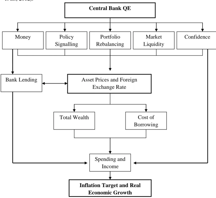
The asset purchases, under QE, push up asset prices by lowering expectations about the future short-term interest rate and reducing the term premium. Higher asset prices increase the net wealth of asset holdings and reduce the cost of borrowing, boosting nominal spending in the private sector, helping to achieve a higher inflation rate, stimulate economic growth, and reduce the unemployment rate. The asset price channel may have an impact through the bank lending and confidence channels: (1) in the bank lending channel, the improvement of liquidity persuades banks to finance more new loan (however, there are restrictions due to the weak financial system); (2) the confidence channel may encourage investment and spending directly or further boost asset prices by reducing the risk premium. The channels which QE may support investment and spending are summarized in Figure 1 below, taken from Hausken and Ncube (2013). The main transmission mechanism between monetary policy instruments (e.g., the official interest rate and the monetary base) and the real economy is the bank

(17)

4 lending channel. However, during the latest financial crisis, the risk aversion by banks increased, leading to the failure of the mechanism and shrinking the credit available to the private sector (Olmo and Sanso-Navarro, 2014). As referred previously, the crisis led to a strong economic contraction worldwide and for this reason, Central Banks announced unconventional monetary policies in order to stimulate the economy (Joyce et al., 2012).

Figure 1 – Transmission Channels of QE

Olmo and Sanso-Navarro (2014) argue that the goal of unconventional monetary policies is also to restore the bank lending channel and after that, to reestablish the other transmission mechanisms. They developed a bank-based model to connect the money stock, interest rates, and real income and highlight the relevance of competition in the banking sector. Central Bank QE Money Policy Signalling Confidence Market Liquidity Portfolio Rebalancing

Asset Prices and Foreign Exchange Rate Bank Lending Cost of Borrowing Total Wealth Spending and Income

Inflation Target and Real Economic Growth

(18)

5

b. The Determinants of Credit to the Private Sector

The private sector is divided in households and non-financial corporation and the access to credit is important in both groups. Families, normally, acquires loans to finance consumer expenses, while firms, do it mostly, to finance investment expenditures. Economic growth has an impact on credit demand, as well as productivity expectations. These two factors are included in the four sets of variables that explain the dynamics of credit allocation:

 Borrowing capacity of households

 Financial conditions

 Financial condition of the borrower

 Structural factors that affect the banking system

Structural factors that affect the banking system are linked with the determinants of credit supply and demand, and according to the literature, the determinants of credit focus on the variables related with the demand for credit, due to the strain in measuring supply variables. Both the determinants of demand and the supply of credit are important variables in the dynamics of credit (Castro and Santos, 2010).

According to the majority of the literature that estimates a long-run relationship between the aggregated value of credit and some macroeconomic variables, the total amount of credit has a positive correlation with GDP and asset prices, while presenting a negative correlation with the interest rates (Egert et al., 2007).

c. The Several Quantitative Easing Programs throughout the

World

i. Quantitative Easing in Japan

The economist Richard Werner was the one introducing the term “Quantitative Easing” (QE) for the first time, also proposing the implementation of this kind of policy in Japan in 1994 (Visconti and Quirici, 2015). Therefore, Japan was the first country to implement an unconventional monetary policy in March 2001 due to the decline in consumer prices, a weak banking system and the expectation of a new recession following the collapse of the global information technology bubble. The first program

(19)

6 lasted for 5 years and other QE programs followed (Bowman et al., 2011). The QE Program aimed to introduce more liquidity in the banking system, keeping the overnight interest rate near zero, encouraging bank lending. Others objectives of the Program were the commitment to maintain interest rates at the ZLB – until the core CPI is above zero – and the purchases of Japanese Government Bonds (JGBs), in order to supply banks with liquidity (Gagnon et al., 2011).

Bowman et al. (2011) estimate panel data regressions, using semiannual data for 137 banks over the period of March 2000 to March 2009. The authors study the effectiveness of the Bank of Japan’s injections of liquidity into the interbank market in promoting bank lending. The authors find a robust, positive and statistically significant effect of QE policy on credit boost to the economy. Ugai (2007) investigates the effect of JGBs purchases under QE on portfolio balance, finding small or insignificant effects on longer-term interest rates, including on corporate bonds. According to the author, the maximum of JGBs hold by Bank of Japan was about 4% of GDP, less than the 12% of GDP increase in the Federal Reserve holdings under the Large-Scale Assets Purchases (LSAP).

After the financial crisis the policy rates in the United States and the UK decreased quickly and the ECB followed since 2009, although the interest rates were kept above 1% until 2012. Subsequently, the ECB cut all its policy interest rates gradually until late 2014. Regarding the BoJ’s policy rates, these have been at the ZLB since the financial crisis, as can be seen in Figure 2 (Driffill, 2016).

(20)

7 Figure 2 - Central Bank Interest Rates

ii. Quantitative Easing in the USA

The Federal Reserve started to increase the balance sheet after the Lehman Brothers bankruptcy, starting the QE1 (2008-2009) buying $600 billion in mortgage-backed securities (MBS). In March 2009 it held $1.75 trillion in bank debt, MBS and Treasury notes. The Fed halted the program after the economy started to improve, however the program resumed shortly, since the economy was not growing vigorously. In November 2010, the Fed announced the QE2 program, buying $600 billion in long-term Treasury Securities (Driffill, 2016). These kind of actions resulted in excess reserves leading to an improvement in the economy as well as in the banks’ opportunities to lend and invest (Thornton, 2012). In September 2012 was announced the QE3 program by the Federal Reserve and the Federal Open Market Committee (FOMC), with monthly purchases of $40 billion of agency mortgage-backed securities in an open-ended program. Three months later, the FOMC announced an increase in the monthly purchases from $40 to $85 billion (Driffill, 2016). -1 0 1 2 3 4 5 6 7 %

Central Bank Interest Rates

Main refinancing rate (ECB, euro area) Federal target rate (Fed, United States) Bank rate (BoE, United Kingdom) Target policy rate (BoJ, Japan)

(21)

8 Using daily data from the Committee on Uniform Securities Identification Procedures (CUSIP)1 on LSAP and returns, D’Amico and King (2010) analyze the effects of changes in the supply of publicly available Treasury debt on yields. The result is a reduction in longer-term Treasury yields, between 30 and 50 basis points, which is large taking into account the historical standards and represents a cut in the cost of borrowing for corporations and households. Therefore, the Treasury LSAP program “was probably successful in its stated goal of broadly reducing interest rates, at least relative to what they would otherwise have been”.

Gagnon et al. (2011) was one of the first studies about the US Federal Reserve’s LSAPs, focusing on the effects on securities’ long-term interest rates. The conclusion is that QE had economically significant and long-lasting effects. The authors found a reduction, between 30 and 100 basis points, in the 10-year term premium, which they estimated to be in the lower and middle thirds of this interval. Moreover, they find a more dominant effect of the interest rates on agency debt and agency mortgage-backed securities (MBS), improving the liquidity of the financial system.

Chen et al. (2011) estimated the effects of LSAP2 on some macroeconomic variables using a dynamic stochastic general equilibrium (DSGE) model incorporating asset market segmentation. The results show that the impact of LSAP2 on GDP growth is not expected to go beyond 0.5%, with a minimal impact on inflation.

iii. Quantitative Easing in the UK

In March 2009 the Bank of England’s Monetary Policy Committee (MPC) announced the program of large-scale purchase of public and private assets – QE - in addition to the reduction of its bank rate to the historical low rate of 0.5%. In the first round of QE, the Bank of England purchased £200 billion of assets, exclusively Government Bonds (Gilts). Later on, the Bank of England purchased more £175 billion, bringing the total amount of the program to £375 billion (Joyce and Spaltro, 2014).

The impact of the initial QE program (2009-2010) on financial markets is analysed by Breedon et al. (2012), taking into account two empirical approaches to measure the

1

According to D'Amico and King (2010) the CUSIP-level data allow us to analyze the effects better. It is possible to examine "differential effects of purchases across security characteristics such as maturity and liquidity".

(22)

9 impact of QE, uncovering an economically significant impact on bond market. The impact of this type of monetary policy on the economy, in particular on financial markets, remains controversial. The study by Joyce et al. (2011), with the identical purpose, found that the medium long-term UK government bond yields fall by about 100 basis points.

Bridges and Thomas (2012) examine the impact of QE on money supply using a “Monetary Approach” and the estimates are applied to two econometric models: (1) an aggregate structural vector autoregression (SVAR) model and (2) a model linked with a set of sectoral money demand systems (a sectoral approach). The authors concluded that an increase of 8% in money holdings, in the QE period, decrease the yields, on average, about 150 basis points, and increased the asset values by 20%. These effects, based on the sectoral approach, led to a boost in the GDP around 2% and in the CPI by about 1%.

Joyce and Spaltro (2014) study the effects of QE on bank lending growth, using new non-publicly available data on UK banks and explore the heterogeneities between large and small banks. The authors found that QE may lead to an increase in bank lending, since the deposit ratio has a statistically significant effect on bank lending. Moreover, the effects on small banks are higher than in the big ones.

d. Quantitative Easing in the Euro Area

In order to respond to the financial and the sovereign debt crises, the ECB implemented some measures to provide liquidity in the economic system. The programs implemented were:

 Long-Term Refinancing Operations (LTROs) in October 2008 – LTROs is a three-month liquidity-providing operation (in euros), one of the two regular open market operations. Through this program, the ECB provides financing to Euro Area banks.

 Covered Bond Purchase Program (CBPP) in May 2009 and 2nd CBPP Program in October 2011 – The purchase of covered bonds helps to improve the functioning of the monetary policy transmission mechanism as well as support lending conditions in the Euro Area.

 Securities Market Program (SMP) in May 2010 – ECB’s interventions in public and private debt securities markets in the Euro Area in order to restore monetary

(23)

10 policy transmission mechanism, making the monetary policy efficient-oriented towards price stability in medium term.

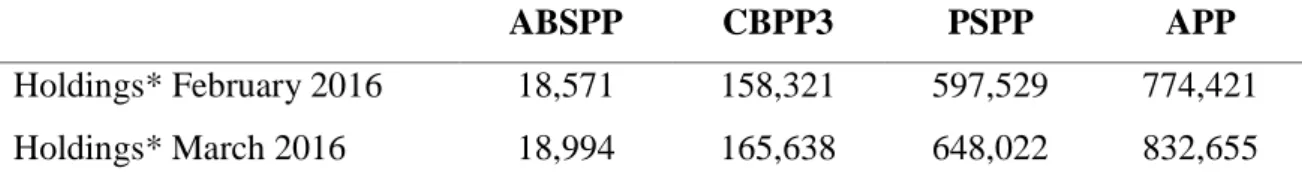
However, none of these programs was enough to provide liquidity and give confidence to the investors about the default risk on the sovereign debt of some countries like Portugal, Spain, Italy, and Greece (Driffill, 2016). So, after the Japan, United States and United Kingdom, it was the turn of the ECB to announce, in September 2014, the Expanded Asset Purchase Program (EAPP), the unconventional monetary policy formally designated by QE. The first announcement and implementation was the Third CBPP and the Asset-Backed Securities Purchase Program (ABSPP). On 22 January 2015, it was announced another type of QE Program, specifically the first Public Sector Purchase Program (PSPP), directed to the purchase of sovereign bonds from Euro Area governments and securities from European supranational institutions and national agencies. Therefore, PSPP was added to the CBPP3 and to the ABSPP, like we can see in Table 1.

Table 1 - QE Announcement and Implementation Dates

Source: ECB

In Tables 2 and 3 is possible to verify that the ABSPP is the smallest of the three programs and the PSPP is the biggest of all instruments (Claeys et al., 2015).

Table 2 - Eurosystem Holdings under the Expanded Asset Purchase Program

ABSPP CBPP3 PSPP APP

Holdings* February 2016 18,571 158,321 597,529 774,421

Holdings* March 2016 18,994 165,638 648,022 832,655

Source: ECB. * - at amortized cost, in euro million, at the end of the month.

Program Announcement Implementation

CBPP3 4th September 2014 20th October 2014

ABSPP 4th September 2014 21st November 2014

(24)

11 Table 3 - Eurosystem Outright Operations

The original guidelines of PSPP correspond to €60 billion worth of monthly purchases until September 2016 with the following purchases allocation: (1) €10 billion per month of asset-backed securities and covered bonds; (2) €44 billion per month of government and national agency bonds (divided in holdings of the ECB and the National Central Banks); (3) €6 billion per month of supranational institutions located in the Euro Area. On the 3rd of December 2015, Mario Draghi announced an extension of the program, leading to changes in the initial guidelines (Claeys and Leandro, 2016). In its website, the ECB claimed that: “The initial program changed in March 2016, changing the monthly amount of purchases from 60 to €80 billion and changing its end to March 2017 or until the Governing Council sees a sustained adjustment in the inflation, which means the observation of at least a trajectory to the inflation target. According to the Governing Council, one of the reasons to announce the EAPP was the historical low rates in most indicators of actual and expected inflation in the Euro Area. This program can stimulate the economy and ease monetary and financial conditions, which makes access to finance cheaper for firms and households.”

The governments of the Euro Area could not implement fiscal stimulus because most European economies are highly indebted and are reducing deficits. So, taking into account the background of “below target inflation, high unemployment, weak growth, high public debt, the unavailability of fiscal policy, and nominal interest rates at rock bottom” the Central Banks have been using unconventional policies (Driffill, 2016). The introduction of QE by the ECB led to a new perspective about the link between monetary policy and financial stability after the ECB clarify that price stability is the

Instrument Reference date Outstanding amount*

CBPP 29 April 2016 19,082

SMP 29 April 2016 114,685

CBPP 2 29 April 2016 8,442

CBPP 3 29 April 2016 172,253

ABSPP 29 April 2016 19,043

Public sector purchase program 29 April 2016 726,521 Source: ECB. * - at amortized cost, in euro million.

(25)

12 main objective of this program, seconded by financial stability. The Vice-President of the ECB has named this as a new separation principle, implying that fiscal dominance

and financial stability dominance of monetary policy should be avoided by the central banks (Constâncio, 2015). Taking into account this principle, Draghi (2015) says that the financial stability risk should be driven by macro-prudential policy instruments. There are some expectations that QE could increase some price bubbles on certain categories of assets, but Draghi (2015) responds that for now the ECB sees no sign of bubbles, only certain situations in specific markets, in which prices grow up fast. However, if bubbles are of a local nature, the macro-prudential instruments are the most appropriate.

The separation principle, referred above, is criticized by End (2015), concluding that the approach of tightening monetary policy for financial stability reasons at the expense of short-term inflation is not an appropriate reaction, since in some countries the inflation rate is far below the target, making this monetary policy infeasible. The author refers that the financial stability should have more weight as a driving force of asset prices. In a regression with quarterly data for the period 1978-2014, 11 advanced economies2 are analyzed and it was found that a decrease in equity prices and an increase in corporate bond rates lower the inflation rate, meaning that asset price developments should be taken into account in monetary policy.

Albu et al. (2014) analyze the impact of the unconventional monetary policy – QE – issued by four major central banks3 on credit risk, in nine countries of Central and Eastern Europe4. In the study is used daily data in an ARMA-GARCH Model and two variables: credit default closing prices and dates of the announcements of QE policies. The range of influence of QE on credit risk, on the analyzed countries, is similar between the ECB and the BoJ. On the other hand, the influence of QE by the Bank of England and the Federal Reserve is lower (and identical between them). Moreover, the QE policies of the ECB and the Federal Reserve, determine both surges and descents in credit risk, while for the Bank of England and the BoJ the leaning of reduction is superior to those of growth.

2_{Advanced economies are the USA, Japan, UK, Germany, France, Italy, Netherlands, Australia, Norway,}

Sweden and Spain.

3

QE issued by The ECB, the Bank of England, the Federal Reserve and the Bank of Japan.

4

Nine countries analyzed: Turkey, Russia, Germany, Poland, Hungary, Ukraine, Austria, Bulgaria and Romania.

(26)

13 In order to analyze the QE’ effects on prices and yields, Driffill (2016) collected the dates of announcements and actions to examine the changes around those dates. The effects are diverse, depending on the date and country in analysis, hence there are countries more sensitive to announcements than others (e.g., the fall in the 10-year Government bond yields was higher in Portugal - 57.75 basis points - than in Germany, France and Greece - 23.20; 15.00, and 5.06, respectively).

Credit to the private sector is a key source of funding for households and non-financial corporations in the Euro Area, as well as a source of valuable information to analyze and forecast economic activity, prices, and monetary developments. The developments of credit in the Euro Area have received little attention. An exception is Calza et al. (2003), who study the demand for loans to the private sector in the Euro Area between 1980 and 1999 with quarterly data. Relative to the empirical model, the authors argue that “the analysis of the demand for loans to the private sector in the Euro Area is limited to a relatively small set of explanatory variables representing general economic activity and the cost of loans”. Consequently, the model is based in the following long-run relation:

In which LOANS is the logarithm of loans to the private sector (in real terms), GDP stands for logarithm of GDP (in real terms), ST denote the real short-term interest rate, and LT represents the real long-term interest rate. The coefficient associated with the GDP is positive (1.457) while with the real short-term and real long-term interest rates are negative (-0.416 and -3.084, respectively). The second coefficient, associated with the real long-term interest rates, is much higher, meaning that interest rates with higher maturities have more impact on loans.

Hofmann (2001) studies the determinants of credit to the private non-financial sector in 16 industrialized countries5, including 8 Euro Area countries, based on a cointegrated VAR (Vector Autoregressive) estimation, over the period 1980-1998, using quarterly data. The outcome of this study is that in the long-run credit is positively linked to real GDP and real property prices and negatively to the real interest rate. The author also

5

16 Industrialized countries: United States, Japan, Germany, France, Italy, United Kingdom, Canada, Australia, Spain, Netherlands, Belgium, Ireland, Switzerland, Sweden, Norway and Finland.

(27)

14 argues that a rise in real GDP affects lending and property prices positively and increases in both credit and property prices, promote real GDP growth.

The EAPP was introduced to improve lending conditions to the private sector (firms and households). From the related literature is possible to claim that there is little evidence on the impact of this policy on lending conditions. This may be due to lack of information about asset purchases and interest rates, while there is ample evidence on bond yields (Blattner et al., 2016). The authors study the effects of the EAPP through new comprehensive loan-level data from Portugal, and find some positive evidence of its impact at banks exposed to QE both via lower prices and larger quantities. Portugal is relevant to the study because both the size of purchases are large relative to the size of the market, suggesting a significant impact of EAPP, and the dependence of the private sector for bank credit is significant, being a good example to study the transmission of QE through the bank lending channel.

3. Data

In this section we will describe our dataset, data sources, and define our variables and time period. Our work aims to analyze the impact of unconventional monetary policy on private credit in the 19 Euro Area countries.6 The choice of this monetary union can be justified by the little evidence on the impact of QE on credit for several economic agents of the member countries, namely households, firms, and the government, when compared with others economies, namely the U.S.A. and the United Kingdom. A panel model is estimated using monthly data, covering the period between January 2008 and May 2016 (101 time-series across 19 cross-sections). With this sample period it is possible to analyze unconventional monetary policies since their beginning, i.e., after the Lehman Brother’s bankruptcy in September 2008.

The dependent variables were taken from the Thomson Reuters DataStream database and are the loans of Monetary Financial Institutions (MFIs) to Euro Area residents, both private and public (TOT) by country and four other variables related to credit, which will be used interchangeably as dependent variables, namely:

6

The 19 Euro Area economies are: Austria, Belgium, Cyprus, Estonia, Finland, France, Germany, Greece, Ireland, Italy, Latvia, Lithuania, Luxembourg, Malta, the Netherlands, Portugal, Slovakia, Slovenia, and Spain.

(28)

15

 Loans of MFIs to Euro Area general governments (GOV);

 Loans of MFIs to households consumer credit (HCC);

 Loans of MFIs to households for house purchase (HIH).

 We have computed the variable HOUSE, which is the sum of the variables HCC and HIC.

All the referred five dependent variables (TOT, GOV, HCC, HIH, and HOUSE) have p-values for the panel unit root tests above the significance level, hence they are non-stationary (see Tables A1, A2, A3, A4 and A5, respectively, in the Appendix).

We have the following independent variables, chosen according to the literature:

 Industrial Production Index (IPI) - IPI is a monthly series that measures output in manufacturing, mining and electric, and gas utilities, presenting values between 0 and 100. The IPI is used as a proxy for the Gross Domestic Product (GDP), which measures the market value of goods and services produced in a country. The source of this data was the Thomson Reuters DataStream database. This variable presented evidence of seasonality in all its cross-sections (countries), which can be seen in Figure A1 in the Appendix. In order to remove the seasonal component we used the X-12-ARIMA procedure, with a multiplicative decomposition. The series after seasonality have been removed are presented on Figure A2. This series was labelled IPI_NS. IPI_NS has a p-value in unit root tests below the significance levels, so it is stationary (see Table A6 in the Appendix).

 EURIBOR (Euro Interbank Offer Rates) – The EURIBOR is based on average interest rates established by a group of around 50 European banks that lend and borrow from each other. We have data for EURIBOR 3 months (EUR03M) and 6 months (EUR06M). The Bloomberg was the database used to get this data. Both variables have p-values lower than significance levels, so they are stationary (see Tables A7 and A8 in the Appendix).

 Risk-Free Rate (GOV10Y) – To represent the risk-free rate we choose the 10-year Government Bond Yield for each country in analysis. Usually, a government bond is issued by a national government and is denominated in the

(29)

16 country’s currency. The source for this variable was the Eurostat. In contrast to the last four independent variables mentioned, GOV10Y is non-stationary (see Table A9 in the Appendix).

 Interbank Offered Rate (INTRATE) – The interbank rate is the rate of interest charged on short-term loans made between banks, which can borrow or lend money in the interbank market in order to control for liquidity. There is a broad range of interbank rates such as: LIBOR (London), LISBOR (Lisbon) and VIBOR (Vienna). These rates are set taking into account the average rates on loans made within that interbank market. Thomson Reuters DataStream database was the source for all these rates. The Interbank Offered Rate is a stationary variable, having low p-values (see Table A10 in the Appendix).

 Inflation Rate (INFL) – The annual inflation rate, in percentage, is measured by the Harmonized Index of Consumer Prices (HICP) and this rate measures the change of the HICP between a month and the same month of the previous year. The source for this variable was the Thomson Reuters DataStream database. The unit root tests for INFL have opposite results. For the Levin, Lin & Chu (2002) and Im, Pesaran & Shin (2003) tests, the variable is stationary, while for the ADF – Fisher and PP – Fisher tests is non-stationary (see Table A11 in the Appendix).

 Quantitative Easing (PSPP) – This variable is the monthly net purchases under the Public Sector Purchase Program (PSPP) by country and data are available since March 2015, when the program started, until May 2016. However, there are no data for Greece and Cyprus presents missing values. The explanation for the absence of data for Greece is that the ECB cannot buy Greek sovereign bonds as part of its QE program. The Greek rating was too low and the Governing Council decided that the countries that have bond yields lower than the deposit rate are excluded from the purchases. In relation to Cyprus, the reason is that it became eligible for the EAPP of the ECB only on October 2015. The negative net purchase in Cyprus in March 2016 is the result of transactions conducted to ensure continued compliance within the limit framework, reflecting buyback operations by the Cypriot Public Debt Management Office.

(30)

17 The source for monthly net purchases was the ECB. The PSPP variable is non-stationary (see Table A12 in the Appendix). In this kind of variables we have to take first differences.

 UNCONV (Dummy) - The dummy was built to capture the effect of unconventional monetary policy on the dependent variables and is the same for all countries. In order to perform an event study, we made a list with monetary policy announcement days (see Table A13 in the Appendix). The dates match announcements dates of unconventional monetary policy initiatives by the ECB. In the same table, there is a column that shows whether conventional monetary policy measures were announced on that same day, i.e., whether there were changes in short-term policy interest rate at the same day. The first announcement by the ECB concerning unconventional monetary policies is on the 28 of March 2008, year of the Lehman Brother’s bankruptcy, representing the start of the financial crisis period. The dummy is defined as follows below.

 CONV (Dummy) – This dummy was built taking into account the changes in conventional monetary policy at the time of regular Governing Council meeting (see Table A14 in the Appendix). The dummy is defined as:

 TT (Dummy) – This variable intends to capture the effect of the period since the ZLB started (February/2012 – May/2016). The dummy is defined as:

 TT3 (Dummy) – This dummy defines the period that the ECB was concerned in controlling for the inflation rate (above the target of 2%). The definition is:

(31)

18

Through the Correlation Matrix between the independent variables (see Table A15 in the Appendix) is possible to determine the possibility of the existence of multicollinearity. We can conclude that the two variables that cannot be simultaneously in the regressions, because the correlation between them is higher than 0.8, is the EUR03M and EUR06M.

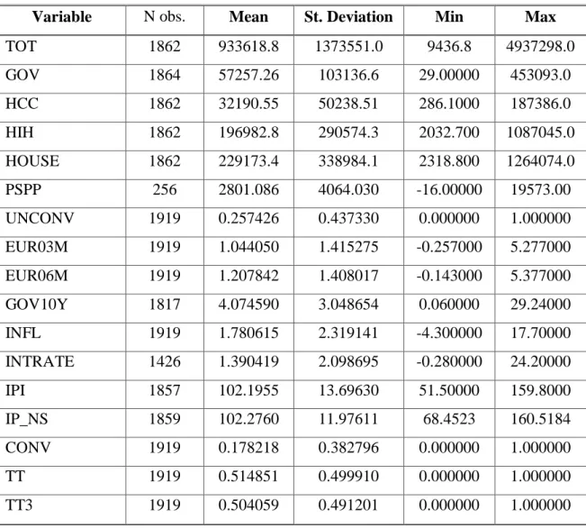
Table 4 presents summary statistics (number of observations, mean, standard deviation, minimum, and maximum) for the dependent and independent variables. Table 5 shows the arithmetic average for the dependent variables, calculated by country (cross-section).

Table 4 - Descriptive Statistics for the Main Variables

Variable N obs. Mean St. Deviation Min Max

TOT 1862 933618.8 1373551.0 9436.8 4937298.0 GOV 1864 57257.26 103136.6 29.00000 453093.0 HCC 1862 32190.55 50238.51 286.1000 187386.0 HIH 1862 196982.8 290574.3 2032.700 1087045.0 HOUSE 1862 229173.4 338984.1 2318.800 1264074.0 PSPP 256 2801.086 4064.030 -16.00000 19573.00 UNCONV 1919 0.257426 0.437330 0.000000 1.000000 EUR03M 1919 1.044050 1.415275 -0.257000 5.277000 EUR06M 1919 1.207842 1.408017 -0.143000 5.377000 GOV10Y 1817 4.074590 3.048654 0.060000 29.24000 INFL 1919 1.780615 2.319141 -4.300000 17.70000 INTRATE 1426 1.390419 2.098695 -0.280000 24.20000 IPI 1857 102.1955 13.69630 51.50000 159.8000 IP_NS 1859 102.2760 11.97611 68.4523 160.5184 CONV 1919 0.178218 0.382796 0.000000 1.000000 TT 1919 0.514851 0.499910 0.000000 1.000000 TT3 1919 0.504059 0.491201 0.000000 1.000000

(32)

19 Table 5 - Arithmetic Mean for Credit Variables by Country (Cross-Section)

Country TOT GOV HCC HIH HOUSE PSPP

Austria 581,525 28,120 23,403 82,035 105,438 1,393 Belgium 545,485 25,681 8,753 96,942 105,695 1,755 Cyprus 71,432 1,045 3,384 11,070 14,454 67 Estonia 16,727 427 663 6,003 6,666 7 Finland 241,019 8,918 12,859 80,272 93,131 892 France 4,208,911 293,635 152,713 796,231 948,944 10,127 Germany 4,602,594 377,981 177,845 995,206 1,173,051 12,759 Greece 270,676 9,696 29,521 71,371 100,892 --- Ireland 494,117 22,672 17,331 94,726 112,057 811 Italy 2,451,557 257,385 60,490 333,906 394,396 8,749 Latvia 18,724 114 792 5,874 6,666 62 Lithuania 18,939 795 852 5,915 6,767 111 Luxembourg 440,803 4,313 1,944 20,438 22,282 106 Malta 14,055 140 371 2,938 3,309 37 Netherlands 1,305,919 52,973 25,036 384,768 409,804 2,839 Portugal 306,501 8,626 13,958 108,078 122,036 1,180 Slovakia 40,205 942 3,114 12,759 15,873 456 Slovenia 35,264 1,285 2,557 4,708 7,265 232 Spain 2,074,302 83,735 76,034 629,434 705,468 6,273

Notes: values in Euro (millions).

4. Methodology

a. Panel Linear Regression Model

In order to analyze the relationship between the amount of credit concession and the net purchases under the PSPP and the announcements of unconventional monetary policy measures, we use an events-study approach through standard panel linear regression

(33)

20 models.7 As explained in the previous section, our work will focus on the 19 Euro Area economies and cover the monthly period between January 2008 and May 2016. Thus, we will develop panel data models, i.e., with both country cross-sectional and time-series dimensions. Our dataset can be regarded as a macro-panel since the number of time periods clearly dominates over the number of countries. Our panel is balanced, with all our cross-section observations valid (no missing values) during the entire time-series period. The general model can be written as follows:

For cross-sections and periods

This KX-dimensional vector represents the “external” explanatory variables, namely

EUR03M and EUR06M. These variables are international, i.e., equal for all countries and cannot be controlled (exogenous).

This KZ-dimensional vector represents the “internal” explanatory variables,

specifically INFL, IPI_NS, GOV10Y, and INTRATE. These variables are determined at each country’s level.

This variable represents the announcements of non-conventional monetary policy. The announcements were transformed in a dummy variable (UNCONV).

This variable (PSPP) represents the amount of purchases through the Public Sector

Program for each country.

This variable (CONV) represents the changes in conventional monetary policy at

the time of the regular Governing Council meeting.

The variable (TT) captures the effect of the ZLB period.

The variable (TT3) captures the effect of the period that the ECB was concern in

controlling the inflation rate (above the target rate of 2%)

7

(34)

21 Represents the intercept. The is the partial slope associated to the jth regressor, after controlling for all other terms.

Is the error term and includes all unobserved components that also affect .

In the general model, we may also include interactions of the announcements dummy variable with other covariates, lags and/or nonlinearities in some particular regressors, and a deterministic time trend.

In order to identify the effect of the EAPP on credit, three different kinds of credit will be considered as the dependent variable : (1) the total loans from MFIs to euro residents; (2) the loans from MFIs to Euro Area general governments; (3) and the total loans from MFIs to households (it includes credit for consumption and for the acquisition of houses).

b. Panel Unit Root Tests and Individual Effects Tests

In macro-panels, the statistical properties of the sample regarding time are relevant for the decision on how variables in the model are to be measured. In particular, stationarity of the series must be tested for so that one can justify using (logs of) levels or first-differences of the observed data and, furthermore, in a cointegration context or not. To that extend, we consider the following panel unit root tests obtained by EViews: Levin, Lin and Chu (2002), Im, Pesaran and Shin (2003), Fisher-type tests using ADF and PP tests – Maddala and Wu (1999). The null hypothesis is of non-stationarity with common or not unit root processes across cross-sections.

In linear regression models using panel data is important to determine the statistical properties of the potential individual-specific effects (country and/or time) – unobservable - which may be correlated with the other observed explanatory variables. The individual country-specific effects are assumed to be time-invariant, fixed or random, distributed independently across individuals and with variance (Hausman and Taylor, 1981). The model’s error is typically decomposed as:

Where can also be added to account for time-specific effects. In this case, and drop out of the model due to collinearity problems. In the LM test, it is assumed that the

(35)

22 unobserved individual effects are distributed as independent and the idiosyncratic disturbances are independent . The null hypothesis is of no individual effects .

Under the null hypothesis, the coefficients are estimated using standard least squares methods. Under the alternative hypothesis, and to know whether the individual effects are fixed or random, it is used the Hausman Test (Hausman, 1978). This test is only applicable under homoskedasticity and cannot include time fixed effects. The random effects (RE) is chosen under the null hypothesis due to its higher efficiency, while under the alternative hypothesis we pick the fixed effects (FE) estimator, the one that is consistent.

Hausman Test Statistic:

Where is the FE estimator for the panel data model with FE errors and is the corresponding RE estimator. The “Cov” terms are the variance-covariance matrices. The limiting law is therefore the chi-squared distribution with k degrees of freedom, where k is the number of coefficients in the model.

(36)

23 Interpretation of the Hausman Test

is true is true

Random Effects (RE) Estimator

Consistent

Efficient

Inconsistent

Fixed Effects (FE) Estimator

Consistent

Inefficient

Consistent

For further details about the estimation and inference of panel data models see, for example, Wooldridge (2006) and Arellano (2003).

5. Results

This study aims to show the contributions of unconventional monetary policies to the loans of MFIs to Euro Area residents (total), as well as disaggregated by Euro Area general government and households, as we have explained above. The results presented were estimated through a regression analysis using a method of Least Squares (LS) and all coefficients are significant and apparently with the expected signs.

The existence of individual effects was tested for all models, concluding that only for GOV does not exist individual effects, since the p-value of the test is above the significance level. For all other models the p-value is close to zero, which means that there are individual effects (see Table 6 below).

(37)

24 Table 6 - Summary of Individual Effects’ Test

Redundant Fixed Effects Test8 Test cross-section fixed effects

Dependent Variable P-values

Cross-section F Cross-section Chi-square

TOT 0.0001 0.0001

GOV 0.9672 0.9658

HCC 0.0000 0.0000

HIH 0.0000 0.0000

HOUSE 0.0000 0.0000

After we have tested for the existence of individual effects, we use the Hausman test to know whether the individual effects are fixed or random. The conclusion is that all models that present evidence of individual effects, have p-values below the significance level, meaning that they exhibit fixed-type effects (see Table 7 below).

Table 7 - Summary of the Hausman Test

Correlated Random Effects – Hausman Test9 Test cross-section random effects

Dependent Variable P-value Cross-section random

TOT 0.0026

HCC 0.0004

HIH 0.0093

HOUSE 0.0012

As explained before, in order to capture the effect of non-conventional monetary policies on Credit, there are two particular independent variables of interest: UNCONV (dummy) and PSPP (level variable). We use these variables interchangeably in the models, but never together, in order to know the impact of each one on credit. We only

8

See all outputs in Tables A16, A17, A18, A19, and A20.

(38)

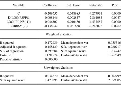
25 use the PSPP variable in the GOV estimations, since this program will have a direct impact in the loans to governments – the biggest percentage of monthly asset purchases by the Eurosystem is allocated to the Public Sector Purchases. So GOV was studied in two ways: first with PSPP and then with UNCONV.

The estimation with PSPP of the GOV model was made with the GLS Weight Period SUR procedure and concludes that, for a 1% increase, ceteris paribus, PSPP and the IPI_NS have a positive impact in loans to Euro Area Governments of 0.00815% and 0.04651%, respectively. On the other hand, for the same 1% increase, ceteris paribus, the EURIBOR 6 months (with a lag of 3 months) has a negative impact of -13.824% (see Table 8 below).

The results presented before were estimated with PSPP as an explanatory variable for the unconventional monetary policy. The following results were estimated with the dummy variable, UNCONV.

An increase of 1% in the IPI_NS causes an increase in credit, ceteris paribus. This impact occurred in five dependent variables, being higher in loans to euro area general governments (0.0666%) than for TOT, HCC, HIH and HOUSE (0.03673%, 0.01148%, 0.01298%, and 0.01225%, respectively). The sign of the coefficient is as expected, since the IPI is a proxy of GDP and according to the literature review this variable has a positive relationship with credit (See Tables 9, 10, 11, 12, and 13 below).

The implementation of an unconventional monetary policy affects positively the amount of loans (credit). One month after the implementation of measures of unconventional monetary policy, there was an increase of 0.401% and 0.339% in total credit (TOT) and in credit to households’ consumer credit, respectively, ceteris paribus. For the other credit variables, the unconventional monetary policy measures (with a delay of three months) have a smaller impact, but still positive, in credit to households’ for purchase house and total households, 0.1304% and 0.185%, respectively, and higher in credit to government, 1.154%, ceteris paribus (See Tables 9, 10, 11, 12, and 13 below).

During the ZLB years, the variation of 1% in EURIBOR 6 months has a negative impact on loans, which varies between -0.283% and -0.586%, ceteris paribus; depending on the kind of loans that is affecting (See Tables 9, 11, 12, and 13). For the case of the governments the interest rate that affects negatively the loans is the

(39)

26 Interbank Offered Rate. The deviation of 1% in INTRATE, during the ZLB years, decreases the loans to government by 2.497%, ceteris paribus (See Table 10 below).

In the case of loans to the households, the inflation’s impact only occurs during the TT3 period (the period that the ECB was concerned in controlling the inflation rate). For a 1% increase, ceteris paribus, the uppermost impact is in HCC, with 0.091%, and for HIH and HOUSE is 0.039% and 0.043%, respectively.

In the case of loans to the euro area governments, the inflation’s impact only occurs during the conventional monetary policy. When the ECB changes the conventional monetary policy (with a delay of the impact in two months), for a 1% increase, ceteris paribus, of inflation, there is a 0.534% increase in loans.

Also during the conventional monetary policy (with a three months delay), for a 1% increase, ceteris paribus, the impact of GOV10Y in the total credit to euro area residents is superior in 1.019%.

Dependent Variable: D(LOG(GOV)) Method: Panel EGLS (Period SUR) Date: 08/16/16 Time: 16:21

Sample (adjusted): 2015M04 2016M03 Periods included: 12

Cross-sections included: 18

Total panel (unbalanced) observations: 175 Linear estimation after one-step weighting matrix

Variable Coefficient Std. Error t-Statistic Prob.

C -0.209555 0.048985 -4.277931 0.0000

D(LOG(PSPP)) 0.008146 0.002847 2.861084 0.0047

LOG(IPI_NS(-1)) 0.046507 0.010480 4.437552 0.0000

EUR06M(-3) -0.138242 0.061658 -2.242072 0.0262

Weighted Statistics

R-squared 0.172939 Mean dependent var -0.035516

Adjusted R-squared 0.158429 S.D. dependent var 0.980717

S.E. of regression 0.899884 Sum squared resid 138.4742

F-statistic 11.91874 Durbin-Watson stat 1.962549

Prob(F-statistic) 0.000000

Unweighted Statistics

R-squared 0.034370 Mean dependent var 0.002799

Sum squared resid 1.423295 Durbin-Watson stat 2.059805

(40)

27

Dependent Variable: D(LOG(TOT)) Method: Panel Least Squares Date: 08/24/16 Time: 17:29

Total panel (unbalanced) observations: 1697

C -0.169442 0.029288 -5.785360 0.0000 LOG(IPI_NS) 0.036733 0.006351 5.783652 0.0000 UNCONV(-1) 0.004009 0.001336 3.001824 0.0027 TT*EUR06M -0.005864 0.002134 -2.747950 0.0061 CONV(-3)*D(GOV10Y) 0.010190 0.001980 5.146360 0.0000 Effects Specification Cross-section fixed (dummy variables)

S.E. of regression 0.023504 Akaike info criterion -4.650442

Sum squared resid 0.925306 Schwarz criterion -4.579962

Log likelihood 3967.900 Hannan-Quinn criter. -4.624348

Table 9 – Final Output for Dependent Variable TOT

Dependent Variable: D(LOG(GOV)) Method: Panel Least Squares Date: 08/24/16 Time: 17:24

C -0.305562 0.135291 -2.258554 0.0241

LOG(IPI_NS) 0.066631 0.029375 2.268339 0.0235

UNCONV(-3) 0.011543 0.006806 1.696075 0.0901

TT*INTRATE -0.024972 0.010611 -2.353384 0.0187

CONV(-2)*INFL 0.005339 0.002357 2.265430 0.0236

(41)

28

Dependent Variable: D(LOG(HCC)) Method: Panel Least Squares Date: 08/24/16 Time: 17:25

C -0.055086 0.027376 -2.012213 0.0443 LOG(IPI_NS) 0.011487 0.005939 1.934320 0.0532 UNCONV(-1) 0.003399 0.001341 2.535480 0.0113 TT*EUR06M -0.005042 0.002132 -2.364571 0.0182 TT3*INFL 0.000905 0.000256 3.528752 0.0004 Effects Specification Cross-section fixed (dummy variables)

Table 11 – Final Output for Dependent Variable HCC

Dependent Variable: D(LOG(HIH)) Method: Panel Least Squares Date: 08/29/16 Time: 16:20

C -0.057995 0.014166 -4.093888 0.0000 LOG(IPI_NS) 0.012975 0.003073 4.221972 0.0000 EUR06M*TT -0.002833 0.001082 -2.619465 0.0089 INFL*TT3 0.000389 0.000136 2.865839 0.0042 UNCONV(-3) 0.001304 0.000690 1.888627 0.0591 Effects Specification Cross-section fixed (dummy variables)