REM WORKING PAPER SERIES
Into the heterogeneities in the Portuguese labour market: an
empirical assessment
Fernando Martins and Domingos Seward
REM Working Paper 076-2019
March 2019
REM – Research in Economics and Mathematics
Rua Miguel Lúpi 20,
1249-078 Lisboa,
Portugal
ISSN 2184-108X
Any opinions expressed are those of the authors and not those of REM. Short, up to two paragraphs can be cited provided that full credit is given to the authors.
market: an empirical assessment
Fernando Martins
Banco de Portugal Universidade Lusíada de Lisboa REM - Research in Economics and
Mathematics, UECE
Domingos Seward
Conselho das Finanças Públicas
March 2019
Abstract
This paper provides a comprehensive study of the heterogeneity in the Portuguese labour market. We use Labour Force Survey microdata covering a complete business cycle, from 1998:1 to 2018:1, to evaluate the labour market attachment of several labour states and assess the most suitable allocation of individuals across statuses. We also evaluate the adequacy of the conventional unemployment criteria. Following the relevant strand of literature on this topic, we apply an evidence-based categorisation of labour market status by exploiting the information on the results of the behaviour of non-employed. To that end, we use multinomial and binary logit models of the determinants of transitions of workers across labour market states to test for the equivalence between non-employed groups. We conclude that heterogeneity is an evident feature of the Portuguese labour market, both between and within the conventional non-employment states. In particular, we find that the status comprising those inactive workers which want work constitutes a distinct state in the labour market and displays a transition behaviour closer to unemployment than to the group of inactive workers which do not want work. Moreover, the classification as inactive workers of individuals which report "waiting" as a reason for not having searched for a job, those individuals who have searched for a job but are still considered to be out-of-the-labour-force, as well as those individuals which are due to start work in more than three months might not be reasonable, since they show considerable attachment to the labour market and we reject the pooling of such states with their counterparts.
JEL: C82, E24, J20.
Keywords: labour market dynamics, heterogeneity, labour force survey, unemployment, labour market slack.
Acknowledgements: We thank David Neves, Pedro Maia Gomes, Pedro Raposo, Lucena Vieira, and Pedro Portugal for valuable inputs, comments, and suggestions. The analyses, opinions and findings of this paper represent the views of the authors and they are not necessarily those of the Banco de Portugal, the Eurosystem, or Conselho das Finanças Públicas. UECE – Research Unit on Complexity and Economics is supported by Fundação para a Ciência e a Tecnologia. E-mail: fmartins@bportugal.pt; dgosseward@cfp.pt
1. Introduction
The recovery from the global financial crisis and the European sovereign debt crisis that followed is mostly complete. At 2.7% per year in 2017, the Portuguese economy is experiencing the strongest growth of real Gross Domestic Product (GDP) of the past 17 years. Likewise, conventional indicators point towards an ever improving and tightening labour market. The employment ratio has increased steadily since the first quarter of 2013 and the unemployment rate is back to pre-crisis levels. Job vacancies have also increased substantially over the post-crisis period as the labour market tightens.
However, in spite of the aforementioned signs of recovery and improving labour market conditions, wage growth remains weak in most advanced countries (OECD (2018)). Portugal has not been an exception. Indeed, whereas the unemployment rate has followed a decreasing path for several years, wage growth remains exceptionally lower than it was before the global financial crisis for equivalent levels of unemployment. This background of low and decreasing unemployment and relatively stable wage inflation has frequently been regarded as a "puzzle" requiring clarification. In particular, it has prompted doubts on the ability of the unemployment rate to accurately capture the slack contained in the labour market (see, e.g. Yellen (2014)).
The definition of unemployment applied in the Labour Force Survey (LFS) only considers individuals without work during the reference week, who have actively searched for a job in the past four weeks, and are available to work in the next two weeks following the interview, as well as those individuals out of work, who have found a job due to start in the next three months. According to the Portuguese LFS, about three million of the working-age population were not in paid work in 2017. From these people, only roughly 1 in 7 satisfied the requirements to be classified as unemployed, with the remaining classified as inactive (thus deemed to be out of the labour force).
The non-employed population appears to be very heterogeneous. While the distinction between the employed and the non-employed is quite straightforward, the boundary between the unemployed and the inactive (and therefore the associated definition of unemployment) is difficult to trace. Some persons classified as inactive can be considered close to unemployment if they have recently searched for a job or if they express desire to work. Other inactive persons do not seem to show any sort of attachment to the labour force and display little marketable skills or desire to work. Most of these groups are less likely to find a job compared to those who have recently become unemployed, but the examination of longitudinal data on worker flows appears to suggest that some subgroups within inactivity are at least as likely to become employed as the unemployed. Moreover, although the chance of transitioning from inactivity to employment is on average lower than it is from unemployment, the comparatively large size of the inactive population implies that these transitions can contribute substantially to the growth in employment, especially
when unemployment decreases during expansions. One implication is that any effort towards measuring the slack in the labour market by dichotomising the non-employed into "unemployment" and "inactivity" should be expected to be unable to comprehensively capture the complexity of labour market activity.
As extensively discussed by Jones and Riddell (1999, 2006), these measurement matters are crucial for several reasons. First, the measurement of unemployment is of paramount importance for economic analyses, since substantial attention is paid even to small variations in the headline unemployment rate and to differences in the rates across countries. Second, much economic investigation focuses on the durations in several non-employment statuses, and therefore the measurement of these spells (especially when they concern multiple categorisation changes within a single spell in non-employment) is central to this research (see, e.g. Clark and Summers (1979)). Third, withdrawal from the labour force and cyclical participation are critical for macroeconomic fluctuations in the labour market, and these factors in turn stem crucially from persons on the margin of the current categorisations (see,
e.g.Barnichon and Figura (2015)). Lastly, the assessment of these measurement
issues may also inform theoretical research on the labour market. In particular, the notion of productive "waiting" for new job opportunities is frequently applied in flow-based macroeconomic analyses of the labour market, replacing the usual notion of active search for work (Hall (1983) and Blanchard and Diamond (1992)). Furthermore, the so-called "stock-flow" matching is often applied, replacing the random matching of workers and job vacancies (see,
e.g. Coles and Smith (1994) and Coles and Petrongolo (2008)). Thus, it is
apparent that many unemployment modelling studies do not fit well with the conventional measurement system which essentially relies on the job search criterion.
Against this backdrop, the aim of this paper is primarily to assess the above-mentioned issues by conducting a comprehensive study of the heterogeneity in the Portuguese labour market, covering a complete business cycle, and using rich LFS microdata from 1998:1 to 2018:1. At the same time, we evaluate the adequacy of the criteria used for the measurement of unemployment. As proposed by Flinn and Heckman (1983) and subsequently extended by Jones and Riddell (1999, 2006), we apply an evidence-based categorisation of labour market status by exploiting the information on the results of the behaviour of non-employed individuals. Therefore, we classify individuals into the same status if they exhibit equivalent behaviour regarding subsequent status. Such an approach is a valuable complement to the conventional categorisation procedures which are essentially based upon reported information and a
priori reasoning (e.g. regarding which actions should be considered to provide
evidence of attachment to the labour market).
This paper is organised as follows. Section 2 develops our motivation, presents relevant theoretical perspectives with labour market slack measurement implications, and provides a literature review about past evidence
on the heterogeneities in the labour market. Section 5 briefly describes the data used in our study and the adopted labour market classification strategy. Section 6 provides a comprehensive empirical assessment of the heterogeneity in the Portuguese labour market: we set out the statistical framework; we present an unconditional assessment; and we report the conditional assessment, including the econometric model, the discussion of the results, and a robustness check. Section 7 concludes.
2. The Measurement of Labour Market Slack
2.1. How good is the unemployment rate as a measure of labour market slack?
The concept of labour market slack can be defined in several ways. For the purpose of this paper, labour market slack is defined as the shortfall between the amount of work supplied by workers and the actual amount of work demanded by employers. It represents the unmet supply of paid work in an economy.
The unemployment rate is the most commonly used proxy of labour market slack. It is defined as the ratio between the number of unemployed individuals over the labour force.
Labour force surveys constitute the main source of data for the estimation of the number of unemployed individuals and their characterisation. Labour statistics split the working-age population into three mutually-exclusive groups: the employed, the unemployed, and the inactive (i.e. the group of individuals deemed to be out of the labour force).
However, while the distinction between the employed and the non-employed is quite straightforward, the boundary between the unemployed and the inactive (and therefore the associated definition of unemployment) is difficult to trace. According to the Portuguese Labour Force Survey (LFS), which follows the general guidelines set by the International Labour Organisation (ILO) and the Eurostat, an unemployed person must fulfil simultaneously three conditions: (i) did not work during the reference week, (ii) is available to work during the reference week or within the next two weeks, and (iii) has actively searched for work during the reference week or within the previous three weeks (or, having not searched, must be due to start work in the next three months).
The classification relies on the degree of attachment to the labour market, based on the job search criterion. However, such a requirement does not necessarily square well with an economic analysis framework. The search criterion is usually not defined with respect to time or pecuniary inputs and, importantly, it does not refer to the characteristics of the job, e.g. the offered wage, that could lead it to be acceptable or not (Jones and Riddell (1999, 2006)). Absent is some notion of whether a specific type of search is suitable for the individual concerned, which may lead the distinction between the
unemployed and the inactive to rely on survey answers containing little or no behavioural substance1.
In addition, the non-employed population seems to be a very heterogeneous group. Some persons classified as inactive can be considered close to unemployment if they have recently searched for a job, if they express desire to work, or if they are about to start a new job but beyond the three-month threshold for an individual to be classified as unemployed. Other inactive persons do not appear to show any sort of attachment to the labour force and display little marketable skills or desire to work. A group classified as inactive which has been the subject of increasing policy concern comprises the so-called discouraged workers, which are those individuals that want to work, but do not actively search for a job. Among the reasons for not actively searching for work is the belief that no work is available. More generally, inactivity includes individuals marginally-attached to the labour force, comprising those individuals that express a desire to work, but do not engage in active search for several reasons. There has been significant debate on the criteria used
to measure unemployment2 and, in particular, on the issue of whether this
marginally-attached group should be treated as inactive as is current practice.3
Even within unemployment the behaviour of the long-term unemployed suggests considerable variations in employability. Indeed, recent resumé audit investigations conclude that short-term and long-term unemployed exhibit substantial differences in the transition behaviour to employment (see Kroft
et al.(2012) and Eriksson and Rooth (2014)).
Unemployment will not be an ideal metric of labour market slack if the requirements do not sort individuals appropriately relative to their willingness to work and/or their likeliness of finding a job, e.g. if considerable fractions of the non-employed, which do not satisfy the requirements to be classified as unemployed, are likely to answer in a similar way when finding a relevant job vacancy.4
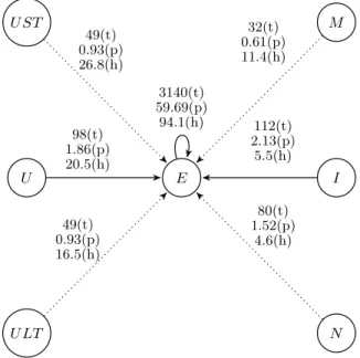
In practice, many non-employed persons become employed without ever being recorded in unemployment. Figure 1 summarises the average quarterly employment inflows disaggregated by several subgroups, over the period from 2012:1 to 2018:1. We observe that indeed employment inflows originating
1. A discussion on this issue is provided in Lucas and Rapping (1969) and Jones and Riddell (1999).
2. This debate is reflected in differences in the criteria that persist between countries, as well as within countries over time (Sorrentino (2000)). Notably, many countries have switched from a concept of unemployment defined in a broad sense (whereby the active search criterion was not considered) to a concept of unemployment defined in a strict sense. For instance, in Portugal the former concept of unemployment was adopted in the survey until 1982.
3. See Cain (1980), OECD (1987), Norwood (1988), Jones and Riddell (1999, 2006) for examples on this discussion.
4. See, e.g. Jones and Riddell (1999, 2006) and Schweitzer (2003) for discussions on these issues.
from inactivity are substantial, and represent on average 112,000 individuals which transition into employment each quarter. This figure compares with an average of 98,000 individuals originating from unemployment, over the period under consideration. In particular, we observe that the transition pattern differs considerably between the inactivity subgroups. Approximately 11% of the marginally-attached (those that express a desire to work) move into employment each quarter on average. On the other hand, the non-attached workers are less likely to transition to employment (only 5% do so each quarter). Still, given the considerable size of the non-attached, such a low transition rate translates into non-negligible gross flows into employment in absolute terms (80,000 non-attached individuals move to employment quarterly). In addition, differences among the unemployed are also noteworthy. As expected, the short-term unemployed are much more likely to move into employment than the long-term unemployed (26.8% versus 16.5%, respectively).
U U ST U LT E I M N 98(t) 1.86(p) 20.5(h) 49(t) 0.93(p) 26.8(h) 49(t) 0.93(p) 16.5(h) 3140(t) 59.69(p) 94.1(h) 32(t) 0.61(p) 11.4(h) 112(t) 2.13(p) 5.5(h) 80(t) 1.52(p) 4.6(h)
Figure 1: Average quarterly worker flows into employment by subgroups, 2012:1-2018:1.
Source: Authors’ calculations based on the LFS.
Notes: the worker gross flows are expressed as total number of individuals in thousands (t), as a percentage of the labour force (p), and as a hazard rate (h). The statistics are the quarterly averages of the period from 2012:1 to 2018:1. U , U ST , U LT , I, M , and N stand for unemployment, short-term unemployment (less than 12 months), long-term unemployment (12 or more months), inactivity, marginally-attached, and non-attached, respectively.
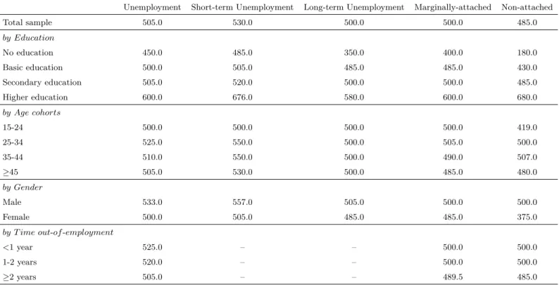
These apparent differences in employability are reflected in the wages earned once these individuals become employed. Remarkably, inactive individuals
which express a desire to work report a median net wage which is comparable to that of the unemployed (500 Euros versus 505 Euros, respectively), and equal to the one reported by the long-term unemployed (see the second line in table B.1 in Appendix B). On the other hand, the reported net wage by those that do not express a desire to work is considerably lower (485 Euros), which is a further indication of the apparent heterogeneity among inactivity. Even though the reported median net wages by the subgroups under consideration reflect similar effects by education, by age cohort, by gender, and by time out-of-employment, in level they appear to mirror substantial differences in employability, as suspected by a preliminary analysis of the transition rates.
The aforementioned subgroups of inactivity are quantitatively relevant and could thus affect one’s perspective on the amount of underutilised labour supply in the market. In our data, the marginally-attached represent roughly 6% of the non-employed population and discouraged workers almost 2% (see table B.2 in Appendix B). Whereas most individuals in these groups have a lower chance of moving to employment compared with the recently unemployed, they often obtain work. Therefore, they can serve to enlarge the pool of unemployed as a potential source of workers.
In sum, the unemployment rate does not capture all relevant forms of labour market slack. Particularly, measured unemployment does not account for slack that might persist within inactivity. Its chief defect is that it relies on a single-boundary conceptual framework, excluding individuals which exhibit attachment to the labour market. Therefore, it does not recognise the substantial heterogeneity in the labour supply and it ignores non-employed individuals which often move into employment.
3. Theoretical perspectives
The classical labour theory is not particularly useful in terms of unemployment measurement implications considering that within this framework the amount of demanded labour by firms equals the amount of supplied labour by workers at a market-clearing wage, i.e. no unemployment arises. This aspect of the so-called Walrasian theory of unemployment has led to the historical understanding of unemployment as (at least partially) a result of disequilibrium phenomena. Even though such terminology has contributed to the debate surrounding the modelling of unemployment, it has not improved our comprehension of the determinants underpinning unemployment or on how
one should measure it.5
5. It is apparent that the assumption set by the classical equilibrium theory of a centralised market wherein labour is traded at a given price does not occur in reality. Regardless, useful economic models need not be realistic, and the Walrasian paradigm is important for the analysis
Much economic analysis of unemployment relies on the distinction between the unemployed and the inactive, with the former often modelled as those that are engaged in optimal search activities and the latter considered to be engaged in household production. The building-block of this approach is based on the observation that the job-finding process is uncertain, requiring time as well as financial resources, which contrasts with the classical model of unemployment, where the intervening agents are assumed to be fully informed at no cost on work opportunities and potential workers (Stigler (1962)). This alternative modelling approach to unemployment is referred to as the
search-theory of unemployment.6It seeks to explain unemployment within a modelling
framework in which an equilibrium rate of unemployment arises as a result of the optimising behaviour of workers and firms, emphasising the frictions associated to the exchange process.
In spite of its atheoretical origins, the view of identifying unemployment with active search has established itself as standard for the measurement
of labour market slack.7 Indeed, most labour market models consider those
individuals classified as unemployed to be willing to work at the prevailing market wage (and therefore located at an "interior solution" regarding the desired hours of work), whereas individuals classified as inactive are modelled as being located at a "corner solution", i.e. in order to enter the labour market they require a higher offered wage.8
On the other hand, flow-based macroeconomic analysis of the labour market frequently apply the notion of productive "waiting" for new job opportunities, which replaces the usual notion of active search for work. In fact, as argued by Hall (1983), in some circumstances, "waiting" might be a productive behaviour regarding the prospects of obtaining work. For instance, the recently unemployed individuals may consider a given stock of job opportunities over which they must search and possibly apply for. As Blanchard and Diamond (1992) put it, "waiting is a more descriptive term than searching" in flow models of the labour market in which separations are a result of job destruction. Furthermore, the random matching of workers and job vacancies is often replaced by the so-called "stock-flow" matching, whereby jobs are created via the matching of the stock or the flow of vacancies with the workers which are available to work (see, e.g. Coles and Smith (1994) and Coles and
of many issues pertaining to labour economics. Still, it is evident that this approach is ill-suited for studying the above-mentioned topics.
6. See Stigler (1962), Diamond (1982a,b), Mortensen (1982), Pissarides (1985), and Mortensen and Pissarides (1994) for notable contributions to this field. For an extensive survey of search-theoretic models of the labour market, see Rogerson et al. (2005).
7. In this respect, Card (2011) provides a discussion on the evolution of the concept of unemployment and its measurement, and how it relates with the existing theoretical constructs. 8. Some examples of research which apply a three-state model for labour market behaviour are: Burdett et al. (1984), Blau and Robins (1986), and van den Berg (1990), among others.
Petrongolo (2008)). The job flows approach assumes that the process of job finding follows an endogenous duration, which ultimately specifies the level of unemployment and wages. Such a theoretical concept is more encompassing than the conventional unemployment conceptual framework, which is chiefly based upon the active search criterion.
Moreover, segmented labour market models such as those presented by McDonald and Solow (1985) and Bulow and Summers (1986) predict that individuals might queue for job vacancies in the primary sector, instead of accepting available job opportunities in the secondary sector. Despite the fact that this behaviour is referred to as "wait" unemployment9 by modellers, in
reality such persons would be classified as inactive in the absence of the conventional search requirement.
Overall, theoretical constructs of labour market do have conceptual implications for unemployment measurement. The conventional criteria for the measurement of unemployment essentially equates its concept with active search, which is broadly consistent with search-theoretic models of unemployment. However, it is clear that many unemployment modelling studies do not fit well with the conventional measurement system.
4. Literature review
The study of the heterogeneity between and within labour market states is crucial for a faithful and comprehensive characterisation of the labour market slack. The literature on transition rates from labour market states into employment with implications for the classification of individuals was started by Clark and Summers (1978). In analysing the dynamics of youth unemployment for the US, the authors claim that most of youth non-employment is not captured by the unemployment statistics, since many stop searching and withdraw from the labour force. The distinction between unemployment and inactive status for youth people might be meaningless, if we consider the wide array of non-market options accessible to youths and limitations imposed by unemployment compensation schemes on the eligibility of this group. The analysis suggests that the empirical distinction between the above-mentioned statuses for this group is considerably arbitrary and of little practical value.
More generally, Clark and Summers (1979) find that transitions between unemployment and employment in the US are considerably lower in magnitude compared with transitions into and out of inactivity. In addition, many individuals appear to experience several changes in classification within a single non-employment spell, with repeated spells of unemployment discontinued by withdrawal from the labour force. Such evidence is supportive of a
weak distinction between the unemployment and the inactive categories. These findings inspired several statistical analyses of the equivalence of the unemployment and inactivity categories.
Flinn and Heckman (1983) test the observation done by Clark and Summers (1978, 1979). Their work is the basis of the subsequent research on this topic. The authors rationalised the distinction between labour market states based on transition probabilities. In this sense, individuals are said to belong to the same labour market state if they exhibit equivalent behaviour with respect
to subsequent labour market status.10 The authors proposed a statistical
framework for testing the behavioural equivalence of labour market states in
longitudinal data, based on a duration of status econometric approach11. Using
the National Longitudinal Survey of Young Men (NLSYM)12, they test for the
equivalence between the unemployment and inactive states for young white American males from the moment they graduate from highschool. They find evidence that rejects this hypothesis. These results are generally in agreement with versions of search theory, whereby unemployment is a state facilitating job search.
Tano (1991) employs the same line of thought, by testing the hypothesis that unemployment and inactive are behaviourally meaningless classifications using the Current Population Survey (CPS) gross flows data. To do so, the author employs a binary logit econometric framework. The results indicate that the two states are distinct for youth, whereas for prime-age individuals they are meaningless. In the same vein, Gönül (1992) extends the former analysis to a wider group of male and female highschool graduates, by employing
a duration econometric model, with mixed results by gender.13 It is worth
pointing out that, in the datasets used by Tano (1991) and Gönül (1992) only the employment, unemployment, and inactive states are observed, which means that they are unable to test for labour market heterogeneity within such states. Jones and Riddell (1999, 2006) extended the former literature by examining the transition behaviour within the unemployed and the inactive groups for the USA and Canada. The authors based their research on labour market status data that enables the identification of the individuals’ expressed desire to work
10. Therefore, two groups may be considered equally attached to the labour market if they are equally likely to move to employment in the following period.
11. In particular, they adopt an exponential functional form in order to model the hazard rates across several labour market statuses.
12. The NLSYM dataset is hampered by the fact that only the duration spells of non-employment and the proportion of the spell spent searching for a job are reported. Flinn and Heckman (1983) tackle this issue by excluding from their analysis all the spells of non-employment spent partly in unnon-employment. Still, such a procedure means that a considerable amount of data is lost and questions the findings’ generalizability.
13. As opposed to Flinn and Heckman (1983), Gönül (1992) does not exclude observations from the econometric analysis, which implies allowing for multiple scenarios in a combinatorial framework, and requiring that some assumptions be put in place, e.g. stationary.
and alternative job search strategies. They examine the equivalence between groups by applying a multinomial logit model for the transition behaviour of individuals. The authors find that the desire to work is a useful indicator for predicting employment in the subsequent period. Accordingly, the group of marginally-attached workers (comprising those inactives that do not search, but want work) is shown to be a distinct labour market state, as well as some subgroups engaged in waiting.
Brandolini et al. (2006) also find evidence of substantial heterogeneity among the inactive group for European countries. The authors investigate the role of the four-week job search requirement by examining the behaviour of those individuals who search for work but did so more than four weeks
before the survey interview.14 The authors’ work is based on the European
Community Household Panel (ECHP), which is a harmonised longitudinal survey coordinated by Eurostat. Their analysis is conducted by a non-parametric equality test. The results show that for most countries this group forms a distinct state in the labour market. In addition, the authors find that these individuals are behaviourally equivalent to the unemployed when their last search effort was done not long before the four-week ILO requirement, which highlights the arbitrariness of the criterion.
In the context of the Portuguese economy, Centeno and Fernandes (2004) studied the heterogeneity of its labour market. The data employed in their work is also drawn from the Portuguese LFS, for the period ranging from 1992:1 to 2003:4. The authors’ methodology follows the seminal work by Flinn and Heckman (1983) in that they adopt a duration econometric framework to model hazard rates. In accordance with previous findings, the results show that
the marginally-attached group is a distinct labour market state in Portugal.15
These findings have subsequently been confirmed by Centeno et al. (2010), with implications for the NAIRU.
Regarding the heterogeneity within the unemployed state, Hornstein (2012) and Krueger et al. (2014) show that even within unemployment the behaviour of the long-term unemployed points towards considerable variations in employability. Indeed, recent resumé audit investigations conclude that short-term and long-term unemployed exhibit substantial differences in the transition behaviour to employment (see Kroft et al. (2012) and Eriksson and Rooth (2014)).
14. Therefore, such workers are not eligible for unemployment.
15. This finding serves as a rough guide to the present work. Even though we adopt a different econometric approach in comparison to Centeno and Fernandes (2004), as well as a longer and more recent sample period, it provides evidence that the Portuguese labour market is also characterised by heterogeneity, at least within inactivity.
5. Data Overview and Classification Strategy
5.1. The Portuguese Labour Force Survey
The Portuguese Labour Force Survey16(LFS) is a household survey conducted
quarterly by Statistics Portugal (Instituto Nacional de Estatística, hereafter INE), with the goal of characterising the Portuguese labour market. The basic structure of the LFS follows the general conceptual, methodological, and precision guidelines set by Eurostat.
The LFS collects individual information on several features pertaining to the labour market, as well as demographic and socio-economic characteristics of the respondents. On the basis of this information, the INE provides quarterly estimates for the stocks of employment, unemployment, and inactivity, which in turn are used for computing several indicators, e.g. the unemployment rate. The richness of the data collected by the LFS allows researchers and policy-makers alike to analyse a wide range of issues related to the labour market.
Every quarter, the INE surveys approximately 40,000 individuals. The population considered in the survey is the group of residents in national territory and the sample unit is the household as main residence. The probabilistic sample of the household units is drawn via the application of a multistage stratified sampling procedure, such that each individual becomes representative of a subgroup of individuals of the population. The sampling procedure ensures an adequate precision at various levels of disaggregation, namely with respect to the regions for statistical purposes (NUTS). Thus, each individual is associated with a given weight, which is then applied for conducting statistical inference to the population.17
The total sample is composed of six sub-samples (i.e. rotations) of individuals, which follow a rotation scheme whereby each quarter 1/6 of the sample is rotated out and 5/6 is kept on the sample. Thus, once selected into the LFS sample, households are interviewed for six consecutive quarters. This feature of the sample allows for the analysis of the data in a longitudinal fashion, because five out of six rotations are the same for every two adjacent quarters. In particular, one can observe the labour force status for 5/6 of the respondents included in the sample in quarters t and t − 1, which enables the computation of worker flows and transition rates.18
We had access to the LFS microdata for the period ranging from 1998:1 to 2018:1.
16. In Portuguese, Inquérito ao Emprego.
17. For further details regarding the sampling procedure and the computation of the weights refer to INE (2015).
18. In practice, we observe less than 5/6 of the sample in adjacent quarters due to non-response. See Appendix A for a discussion on this issue.
5.2. Algorithm for status classification
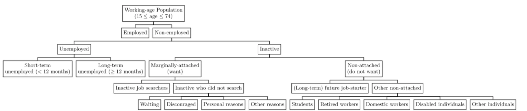
The LFS data are exceptionally rich in the information supplied regarding the methods of job search, reasons for inactivity, and present activities of the non-employed, which enables to generate subgroups of non-employment potentially available to take on work. The adopted classification strategy considers several factors: (i) the findings obtained by the previous literature, which highlight the importance of an expressed desire to work by the inactive individuals as a predictor of future employment; (ii) the structure of the Portuguese LFS questionnaire; (iii) the goal of assessing the heterogeneity in the Portuguese labour market and the classification criteria followed by the INE; and (iv) sample size considerations. It results in a combined categorisation of the non-employment state into 13 mutually-exclusive and exhaustive categories. The adopted classification is summarised in figure B.1 in Appendix B.
We classify individuals in working-age into four states: employment (E), unemployment (U), marginal-attachment (M), and non-attachment (N). The employment and the unemployment states coincide with the conventional classification in the LFS. The latter two states, M and N, are obtained by disaggregating the usual inactivity state according to the wanting criterion. Assignment of the marginal attachment group relies on the LFS question "Would you like to obtain a job?". Those individuals classified by the LFS as inactive which answer "Yes" to the mentioned question are assigned to the
M group. Since only those individuals that did not search for work answer the
question, we also classify inactive individuals that did search for work into M.19
The remainder are assigned to the N group.
Based on the LFS, we perform the conventional split of U according to duration into short- (less than twelve months) and long-term (twelve or more months) unemployed. We further disaggregate the M group into those that searched and those that did not search for work. The latter comprises four subgroups according to reasons for not searching: workers waiting for recall (which includes temporary layoffs), discouraged workers (which indicate economic reasons for not having searched20), workers not searching for personal
reasons21, and workers indicating other reasons for not searching22. Within the
N group, we make a distinction between persons who have found a job due to
start in more than three months (to which we refer to as long-term future job starters) and the remainder; the latter are divided into demographic groups:
19. We do so in order to ensure that the four states considered in our model are both mutually-exclusive and exhaustive.
20. These include individuals that believe that no jobs are available, search is not worthwhile, do not know how to search, consider themselves too young/old or do not have enough education. 21. Namely, due to sickness, looking after family, or other personal reasons.
students, retired workers, domestic workers, disabled individuals, and other individuals.
6. Heterogeneity in the Portuguese Labour Market
6.1. Statistical framework
The literature often relies on multi-state stochastic frameworks in order to analyse the dynamic features of longitudinal data. The adopted statistical framework folows the seminal contribution by Flinn and Heckman (1983) and subsequently extended by Jones and Riddell (1999, 2006) in focusing on transition rates to assess the equivalence between states and the extent of heterogeneity in the labour market.
Let Yt be a random variable describing the status of persons in the labour
market at quarter t. For the purpose of this work, Yt is assumed discrete
and takes on values corresponding to k mutually-exclusive and exhaustive states. We assume that the transition of workers among labour market states is represented by a discrete Markov chain of order 1. Therefore, the data generating process, {Yt}Tt=1, follows:
P r(Yt= i|Yt−1, Yt−2, . . . , Y1) = P r(Yt= i|Yt−1) (1)
wherein i = 1, 2, . . . , k indexes the observed status in the Yt domain. The
process represented by equation (1) is said to respect the Markov property23.
Thus, the observed values for Yt depend only on the current status. In other
words, all other past values for the random process are irrelevant for the determination of future conditional transition probabilities.24
The probabilities of transition from state i to state j over time periods t − 1 and t are given by:
pij,t = P r(Yt= j|Yt−1= i), i, j = 1, 2, . . . , k (2)
Consistent with the adopted status classification presented in section 5.2, we
start by considering four broad labour market states, i.e. k = 4.25The number
of employed, E, unemployed, U, marginally-attached, M, and non-attached, N, then satisfy the following system:
23. In the analysis of labour market dynamics, such assumption is rather strict and whenever possible should be tested. This issue is addressed in subsection 6.3.3.
24. In this sense, the process is said to be "memoryless".
25. It should be noted that the flexibility of the statistical framework allows for the generalisation to any k labour states. This is important to evaluate the heterogeneity within the conventional labour states.
E U M N t = Pt E U M N t−1 (3) The dynamic model can be summarised by the four-by-four transition
matrix P , where the ijth element of the matrix, p
ij, represents the probability
of a person moving from state i ∈ {E, U, M, N} in the current period to state j ∈ {E, U, M, N }in the following period:26
Pt= pEE pEU pEM pEN pU E pU U pU M pU N pM E pM U pM M pM N pN E pN U pN M pN N t (4) In this paper, we apply an evidence-based categorisation of labour market status by exploiting the information on the results of the behaviour of non-employed individuals. Therefore, we classify individuals into the same state if they exhibit equivalent behaviour regarding subsequent status. For instance, one may consider two groups to be equally attached to the market if they are equally likely to move to employment in the next period. The approach we take generalises this idea to all the statuses considered.
Considering this Markovian framework, a necessary and sufficient condition for states M and N to be behaviourally equivalent is that the probability of moving from state M to E is equal to the probability of moving from state
N to E and the probability of moving from state M to U is equal to that of
moving from state N to U:27
(
pM E = pN E
pM U = pN U
(5) If the above condition holds, it is reasonable to pool the M and N states into a single inactivity state, i.e. our four-state model of the labour market collapses into the conventional model (E, U, and I). With regards to equation (5), the wanting-a-job criterion would not convey any useful information on labour market status of individuals.
The opposite scenario occurs if information provided by the job search question does not convey information on the labour market status. In other words, the M and U groups are behaviourally equivalent. Such a result would support the view that the traditional job search requirement for unemployment
26. The matrix Ptis said to be a stochastic matrix considering thatPkj=1pij,t= 1, ∀i, j, t.
Consequently the transition probabilities in each row must sum up to unity.
27. Note that the equivalence conditions relate only exit rates into states other than the origin states under consideration.
classification is too strict. The necessary and sufficient conditions for this case to hold are: ( pM E = pU E pM N = pU N (6) If M is found to be behaviourally distinct from both the U and N states, i.e. if conditions (5) and (6) do not hold simultaneously, we might expect that the attachment pattern between the states follows some kind of order, for example:
pU E > pM E> pN E (7)
From the point-of-view of the LFS data collection methodology, such a finding would suggest the inclusion of the wanting-a-job question as a criterion for status classification.
6.2. Unconditional assessment
In this section, we study the heterogeneity in the Portuguese labour market by analysing the features of the estimated transition rates from the empirical matrix (4). The algorithm constructed for the estimation of the transition rates utilises the rotation scheme of the LFS, which allows to match individual’s responses in one quarter to their labour market outcomes in the subsequent quarter. The algorithm is described in detail in Appendix A.
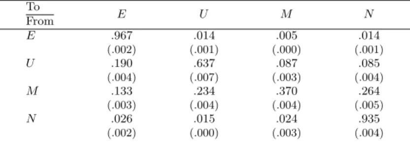
Table 1 shows the estimated transition rates for adjacent quarters averaged across the sample period. For transitions into E, there is a noticeable difference between U and M as origin states, with the transition rate from U at 19%, 6 percentage points above that of M (roughly 13%). Moreover, there is a striking difference between the M and N origin groups, with the transition rate from N to E averaging only 2.6%. The standard errors of the estimated transition probabilities are small (considering the LFS large sample size), such that equality of the means would be easily rejected by a formal statistical test. Moreover, for each non-employment destination state, the transition rates between origin groups U and M and between M and N differ considerably. For transitions into U, the average transition rate from the M group is 23.4%, which
is much higher than the estimated transition rate ˆpN U (at only 1.5%); whereas
for transitions into N, the ˆpM N averages approximately 26.4% in comparison
to 8.5% for ˆpU N.
It is worth pointing out that, judging from the results obtained for the empirical transition matrix, a person who wants to work appears to behave differently from one that does not want to work. First, someone who expresses a desire to work (M) is likely to enter the labour force in the next quarter
(ˆpM U + ˆpM E = 0.37). Equivalently, a person who wants to work can be
considered at the margin of participation. In contrast, a person who does not want to work (N) is very unlikely to enter the labour force in the next
quarter (ˆpN U + ˆpN E = 0.04) and is therefore quite far from labour force
activity and the margin of participation. Second, a marginally-attached non-participant has a higher chance of entering the labour force via unemployment than via employment (i.e. ˆpM U > ˆpM E), but the opposite occurs for a
non-attached person, since it is much more likely to move into the labour force via employment (i.e. ˆpN E> ˆpN U). To From E U M N E .967 .014 .005 .014 (.002) (.001) (.000) (.001) U .190 .637 .087 .085 (.004) (.007) (.003) (.004) M .133 .234 .370 .264 (.003) (.004) (.004) (.005) N .026 .015 .024 .935 (.002) (.000) (.003) (.004)
Table 1. Average quarterly transition rates, 1998:1-2018:1.
Source: Authors’ calculations based on the LFS.
Note: Standard errors in parentheses; The observations from 2010 through 2011 are not considered in the sample to avoid biases resulting from the methodological break of the LFS.
The diagonal elements (ˆpU U, ˆpM M, and ˆpN N) are numerically substantial
and their analysis suggests that M is the least stable group over time, with an estimated 37% probability of an individual remaining in M from one quarter to the next, while N appears to be an absorbing group: at a retention rate of almost 94%, it is by far the most stable.
The examination of the time-series of the transition rates over the sample period (see figures B.2 in Appendix B) confirms to a large extent the behaviour observed for the average transitions obtained for the empirical matrix. Several features should be mentioned. First, the transition rates exhibit in general considerable stability over time, with the exception of the transitions into employment, for which the cyclical pattern is very marked. Second, the ordering of the transition rates is the same in every single quarter over the sample period, with ˆpU E > ˆpM E> ˆpN E, ˆpU U> ˆpM U > ˆpN U, and ˆpN N > ˆpM N > ˆpU N.
Moreover, the difference between ˆpU E and ˆpM Eis consistently much lower than
the difference between ˆpM E and ˆpN E. The fact that ˆpM E is close to ˆpU E is an
indication that an expressed desire to work among non-participants conveys substantial information about their attachment to the labour market.
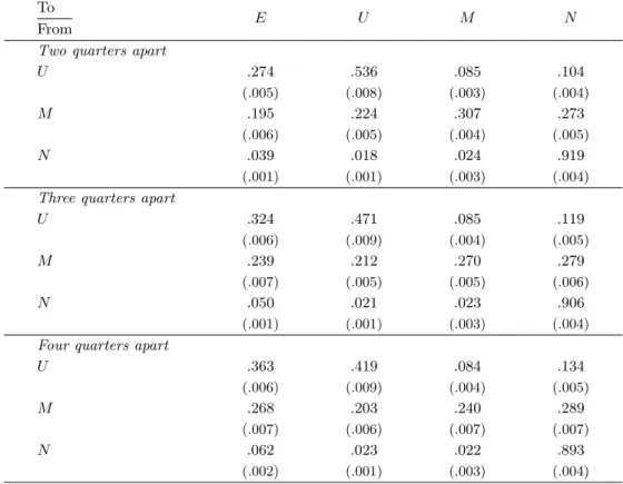
For robustness, we also examine the effect of horizon lengthening on the average transition rates.28The results are reported in table B.3 in Appendix B.
We find that, at each time interval between destination and origin quarters, the
28. This is done by matching individuals over longer time intervals. For example, by matching an individual in a given quarter to the same individual two quarters ahead.
above-mentioned transition regularities are maintained. All the transition rates into E increase at longer time spans, but the ordering ˆpU E > ˆpM E > ˆpN E is
consistent throughout. In general, the standard errors increase as the respective sample size decreases, but the differences are still statistically significant even at 4-quarter horizons.
The other elements of the empirical transition matrix also exhibit coherent behaviour as we increase the time span. The diagonal elements (ˆpU U, ˆpM M, and
ˆ
pN N) decrease at longer horizons, since mobility increases over time, although
the impact is more noticeable for the U and the M rates. One can also observe that the hazard from U to inactivity increases slightly as we move to longer horizons. Importantly, the ordering of the estimated transition probabilities clearly holds, which further confirms the above results.
In order to examine the extent of heterogeneity within the labour market states considered, we also compute the average transition rates by detailed origin state (see table B.4 in Appendix B). We perform the conventional split of U by duration into short-term and long-term unemployed. As expected, the short-term unemployed are almost twice as likely to move into E (25%) relative to the long-term unemployed (14%). Conversely, the long-term unemployed have a higher chance to remain unemployed or to transition to inactivity in the following quarter.
Furthermore, we find important heterogeneity within the M group. The striking result is that the "waiting" subgroup, which averages 23.33 thousand individuals quarterly over the sample period (approximately 12% of the M) -see table B.2 in Appendix B - shows a transition rate into E considerably higher than the other subgroups of M. This category displays an average hazard of 28.8% (see table B.4), exhibiting quarterly rates in excess of 50% (see figure B.3 in Appendix B), as opposed to the other four subgroups that average in the range from 9% to 16%. As reported in table B.4, the higher hazard into
E coexists with a much lower hazard into N, i.e. the waiting subgroup is
not only more likely to transition into E, but also less likely to become non-attached. Moreover, those M individuals which report having searched for a job, which amount to roughly 14 thousand individuals quarterly on average (corresponding to 7% of the M), also display significant attachment to the labour market. In particular, approximately 16% of these individuals move to employment quarterly on average, which is above the transition rate of the long-term unemployed (14%). Despite this, such individuals also move often to
N (19% do so each quarter on average), which is still considerably below the
corresponding transition rate displayed by most of their M counterparts. A further set of measurement issues we aim at addressing arise for persons which do not search for work but have found a job due to start in more than three months (or within three months, but do not meet the availability criterion), to which we refer to as long-term future job starts. In Portugal, as in many other countries, such persons are classified as inactive. Therefore, statistical agencies treat this subgroup in a different way relative to those that
have found a job due to start within three months and are available (which do not need to fulfil the job search criterion to be categorised as U). This subgroup of N amounts to 1.44 thousand individuals quarterly on average over the sample period in consideration (see table B.2 in Appendix B). The last panel of table B.4 presents the hazards for this group, as well as for the remainder of the non-attached group. We find that long-term future job starts display the largest hazard into E of all subgroups considered: approximately 39% move into employment on average every quarter. However, they also exhibit an almost as high hazard into inactivity, which makes it hard to evaluate this classification practice based on these unconditional data. Still, it is apparent that long-term future starts display very different transition behaviour in comparison with other non-attached workers.
In sum, these unconditional data suggest that the U, M, and N groups exhibit considerably distinct behaviour. It appears that the behaviour of the
M is closer to that of the U than to the N, but the U and the M groups
may nevertheless be distinct labour market states.29 Accordingly, we find that
searching for a job and an expressed desire to work among non-participants conveys substantial information about a person’s attachment to the labour market, as pointed out by Centeno and Fernandes (2004) and Centeno et al. (2010).
We also find substantial heterogeneity within labour market states. In particular, the short-term and the long-term unemployed display substantially different transition behaviour. Moreover, the waiting subgroup of M shows stronger attachment relative to the remainder that express desire to work. In fact, on the basis of the empirical transition rates to employment, the waiting subgroup of M is more attached than the unemployed. Those individuals classified as inactive, but who have nevertheless searched for a job, also appear to be more attached to the labour market than their M counterparts, exhibiting transition rates into E in excess of the long-term U. Likewise, the long-term future job starts appear to be much more attached to the labour market than
their non-attached counterparts.30
6.3. Conditional assessment
The findings obtained for the unconditional transition rates are informative, but must be treated with caution. The average transition rates analysed consider persons who differ on various characteristics. Therefore, it is crucial to assess whether the findings are essentially due to compositional effects, such that different types of persons are more or less likely to belong to different groups
29. Such a conclusion would support the view that M is an intermediate state, lying in between U and N .
30. The differences are quantitatively large and consistent with previous evidence found by Jones and Riddell (1999) for the USA and Canada.
than others, with an impact on the respective transitions, or whether the findings still hold after controlling for such differences. A conditional assessment is thus called for. In this section, we specify the econometric apparatus used for this assessment. We then present and discuss the results. Finally, we address several limitations of the adopted specification by performing a robustness check.
6.3.1. Econometric model. We estimate multinomial logit models (MLM)31of
the determinants of transitions across several employment and non-employment
states.32 Such models will enable us to test whether two origin states are
equivalent controlling for the observable characteristics of the individuals. This amounts to testing the conditional versions of the restrictions (5) and (6) presented above.
The choice of modelling transition rates through MLM, as opposed to alternative longitudinal frameworks is due to two reasons. The first reason is related with the potential issue of attrition. A longitudinal framework is more associated with persistence and is more sensitive to attrition. However, the current analysis is more concerned with recurrence, since any transitions across time periods are under consideration despite potential problems of attrition33.
Second, since the main focus of this work is on non-employment groups in which duration is not well measured, we consider that this econometric approach is preferable to employing a duration modelling framework (as have done,
e.g. Flinn and Heckman (1983) and Gönül (1992)), because we refrain from
additional assumptions regarding the functional form of the model. The individual conditional transition probabilities are as follows:
pij,h,t= P r(Yh,t= j|Yh,t−1= i, xh,t), h = 1, 2, . . . , n (8)
where h indexes the person, Yh,t denotes the first-order Markov chain for
person h at time t, and xh,t refers to any vector of conditioning individual
characteristics. The labour market states are constructed such that they are both mutually-exclusive and exhaustive. Therefore, the probabilities add up to unity for each individual h, i.e. Pk
j=1pij,h= 1, ∀h.
The simplest approach to the MLM is to define one of the outcome categories as a baseline, compute the log-odds with respect to the baseline category, and then let the log-odds be a linear function of the covariates. As such, the probability of moving into a category is compared to the probability
31. For an overview of the multinomial logit class of models, see Greene (2012) and Hosmer
et al. (2013).
32. As opposed to Jones and Riddell (1999, 2006), we report the results from pooled multinomial logit regressions, since it has the advantage of increasing the sample size. We have also estimated the same set of models for each of the transitions quarterly, with very similar results.
of membership in the baseline category. Considering that, in the most general case, we have k categories, such an approach requires the computation of k − 1 equations, one for each destination state with respect to the baseline. Thus,
there will be k − 1 predicted log-odds. If we define the j∗ as the baseline
outcome, we obtain the following system: fj(xh,t) = ln
P r(Yh,t= j|Yh,t−1= i, xh,t)
P r(Yh,t= j∗|Yh,t−1= i, xh,t)
= αj+ x0hβj, j 6= j∗ (9)
Where αj denotes a constant and βj denotes the vector of regression
coefficients. According to the MLM, the predicted transition probabilities can be expressed as follows: pij,h,t= exp{fj(xh,t)} Pk j=1exp{fj(xh,t)} , if j 6= j∗ 1 Pk j=1exp{fj(xh,t)} , if j = j∗ (10) Since fj∗(xh,t) = 0, we obtain exp{fj∗(xh,t)} = exp{0} = 1. In our model,
we set j∗= i, i.e. we define the baseline outcome as the individual remaining
in the previous state. The model is estimated via maximum likelihood procedure.34
A variety of transition probability tests can be executed through tests on the comparison of coefficients. In particular, likelihood ratio tests can be implemented for some alternative imposed as a restriction on the vector of coefficients.
We aim at testing for the equivalence between the probabilities of transitions into different labour market states, for instance, to test whether one can pool individuals originating from state M with individuals originating from state
N. To do so, we take all individuals in our sample which occupy the M or
N state in the first period, such that their three destination outcomes are E,
U, or to remain in the pooled inactivity state, and we run a multinomial logit
regression, as in equation (9). The covariates refer to the personal and socio-economic characteristics of the respondents, as well as to a set of seasonal and
regional dummy variables35 (see table B.5 in Appendix B).
Afterwards, an unrestricted model is estimated, by adding a dummy variable identifying the individuals which were originally in state M. The origin state dummy is interacted with each explanatory variable. Therefore, the unrestricted model allows for distinct intercepts and influences of the
34. The maximum likelihood estimator, ˆβj, is consistent, asymptotically efficient, and
normally distributed. See Greene (2012) for a proof.
35. Seasonal dummy variables are added because the seasonal behaviour of the transitions is very marked, which might distort our conclusions if not appropriately accounted for.
conditioning characteristics of the individuals, depending on their origin state,
i.e.distinct transition behaviour for individuals who originate from M and N.
In order to test for the equivalence between M and N, i.e. condition (5), we employ a likelihood-ratio test, which compares the maximised values of the logarithm of the likelihood function under the null hypothesis of equivalence between groups and under the alternative hypothesis that the groups are different36.
The same reasoning is applied to test whether there is statistical evidence supporting the equivalence between the M and the U states on the basis of their transition rates, i.e. to test for the condition (6), as well as for testing the equivalence between other subgroups of non-employment.
In practice, the adopted methodology assesses whether two origin states provide sets of coefficients which are statistically significantly equal to each other. In other words, we test whether one should pool together the two origin states, by applying a joint model for the respective transition probabilities. On the one hand, in the case that the coefficients are found to be significantly equal, such that the states can be pooled without any information loss, then we conclude that the states under consideration are equivalent. On the other hand, if the sets of coefficients are found to be statistically different at some suitable significance level (i.e. we reject pooling the states together), we infer that the states should be considered distinct.37
Since the LFS was subject to a survey redesign in the first quarter of 2011, we are forced to conduct the tests separately for each survey. The results will enable us to assess the extent of heterogeneity in the Portuguese labour market.
6.3.2. Discussion of results. The results of the above-mentioned
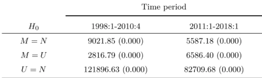
likelihood-ratio tests for the pairwise equivalence between the U, the M, and the N groups are reported in table 2. For each test, the observed value of the test-statistic and the respective p−value are presented. Given our interest in the equivalence tests rather than on the interpretation of the estimated MLM regressions, we
relegate the corresponding MLM estimations to Appendix C.38
We evidently reject the equivalence between M and N, M and U, and
N and U, both in the first and second LFS series. This finding can be
36. The corresponding test statistic follows a chi-squared distribution with degrees of freedom equal to the number of restrictions imposed under the null, if the null is true (Greene (2012)). 37. Despite its convenience, the adoption of a multinomial logit econometric framework raises the concern over the independence between the possible transition outcomes, e.g. whether the relative rates of transition into employment and unemployment would change if the outcome to remain in the marginally-attached and non-attached pooled state were removed. We address this issue in subsection 6.3.3.
38. The estimated regressions are too numerous to report here. We only report those estimations concerning the equivalence between U , M , and N . The remainder are available upon request. We highlight that the majority of the estimated coefficients are significant at the usual significance levels.
Time period
H0 1998:1-2010:4 2011:1-2018:1
M = N 9021.85 (0.000) 5587.18 (0.000) M = U 2816.79 (0.000) 6586.40 (0.000) U = N 121896.63 (0.000) 82709.68 (0.000)
Table 2. Multinomial logit likelihood ratio test for the equivalence between non-employment states.
Source: Based on LFS data.
Notes: The reported values are the observed likelihood-ratio test statistics for the respective H0. The p−values are reported in parentheses.
inferred from the large values for the observed likelihood-ratio test statistic and the respective p−values equal to 0.000 for all the conducted tests. Such results provide evidence supporting the hypothesis that the group comprising marginally-attached workers is distinct from the non-attached, on the basis of the full multinomial logit model, as well as rejecting the equivalence between the marginally-attached group and the unemployed. Furthermore, we decisively
reject the pooling of the unemployed and the non-attached groups.39 Hence,
these formal statistical tests, which account for the observed differences of the individuals in each state, generally corroborate the evidence found for the unconditional assessment.
We also test the heterogeneity within the groups of unemployment, marginal-attachment, and non-attachment (see table B.6 in Appendix B). For the unemployed, our results point towards a rejection of the equivalence between the short-term and the long-term unemployed. In addition, within the marginally-attached, the statistical evidence leads to a clear rejection of the equivalence between its subgroups. Finally, within the non-attached group, we test and strongly reject the null of equivalence between future job starts and
other non-attached.40
Lastly, we conduct statistical tests of two equivalence hypotheses which compare subgroups across the conventional classification criteria. As depicted in figure B.3 and table B.4, there is substantial heterogeneity within the marginally-attached. It is apparent that those marginally-attached which report "waiting" (M(W )) as a reason for not searching exhibit higher transition rates to employment relative to the other subgroups and, importantly, relative to the unemployed. The heterogeneity within non-attachment is also
39. Such a hypothesis was much less plausible from the unconditional analysis.
40. Such a finding is not at all surprising considering the markedly different empirical transition rates observed for these subgroups.
noteworthy, since future job starts (N(F JS)) display on average transition rates to employment above the unemployed, and clearly above those of
other non-attached individuals.41 These observations provide a prima facie
for investigating whether such non-employment states are equivalent to the unemployed. Table B.7 in Appendix B reports the results.
The tests again lead us to reject equivalence between all the states considered. However, one can argue that, to the extent that the tests reject
pooling the states, it is mainly due to pM (W )E > pU E than the other way
around. The same conclusion can be inferred for those future job starts classified as non-attached. Such findings might indicate that the adopted criteria for unemployment lacks empirical foundations. Particularly, in Portugal, the classification as inactive workers of non-employed individuals which indicate waiting and future job starts might not be reasonable.
6.3.3. Limitations and robustness check. We recognise that the adopted
statistical framework is hampered by several drawbacks. The MLM specification implicitly imposes the independence of irrelevant alternatives assumption (IIA) (see Luce (1959)). Under this strong assumption, the relative probabilities of transitions into, e.g. E and U, would not change given the removal of the (irrelevant) alternative of transitions into inactivity. Such a scenario seems unrealistic considering that U is in one sense closer to inactivity than to E.42
Hausman and McFadden (1984) developed a Hausman-type test of the
IIA43. We conduct this IIA test for the multinomial logit models applied for
the equivalence between M and N, and M and U44; the results are reported
in tables C.5 and C.6 in Appendix C, respectively. We obtain mixed results
41. As already noted, the group comprising future job starts also exhibits low probabilities of staying in non-attachment vis-à-vis the very high retention rate of non-attached individuals. 42. This modelling issue had been raised by Jones and Riddell (1999)
43. An alternative test of the IIA has been proposed by Small and Hsiao (1985). We choose to report the Hausman-McFadden tests because the Small-Hsiao test relies on the creation of random half-samples from the data, which implies that results may differ considerably for successive calls of the test; nonetheless, both tests provide mixed results in our data.
44. The test comprises the following stages. First, we estimate the full model with k possible outcomes and the respective estimates are included in bβF. Second, we estimate a restricted model by removing one of the possible outcomes and the respective estimates are included in
b
βR. We proceed to determine bβF∗, a subset of bβF obtained by removing the coefficients which
are not considered in the restricted model. The test is then based on the following test statistic: QIIA= ( ˆβR− ˆβF∗)
0
[ dV ar( ˆβR) − dV ar( ˆβF∗)]−1( ˆβR− ˆβF∗) (11)
which follows asymptotically a chi-square distribution with degrees of freedom equal to the number of coefficients contained in ˆβR, if the null of IIA holds. A significant value for
Q constitutes evidence against the IIA. Hausman and McFadden (1984) note that the test-statistic might assume negative values if dV ar( ˆβR) − dV ar( ˆβ∗F) is not a positive semi-definite
for each outcome, which depends on the category omitted from the full model. Therefore, we cannot rule out the presence of IIA in the multinomial logit models.
To assess the robustness of our results, we thus estimate binary logit models, which can be viewed as imposing the polar assumption of complete
dependence.4546
The statistical framework resembles the one outlined in section 6.1, only that the transition matrix now becomes:
Pt= pE,E pE,E pE 1,E pE1,E pE 2,E pE2,E ... ... pE 13,E pE13,E t (12)
where E denotes the non-employment state and the 13 non-employment mutually-exclusive subcategories are identified from E1 to E13. For the sake of
simplicity, the outflows from E and transitions across non-employment states are ignored.
As noted previously, we are interested in hypotheses pertaining to comparisons to the unemployment group. For instance, we aim at assessing whether the transition rate from the inactive subgroup which states "personal reasons" for not searching is comparable to the one of the unemployed, ceteris
paribus. From a practical point-of-view, it is also relevant to check whether the
estimated transition rate is higher for some subgroup of inactivity relative to the unemployed.
We take advantage of this statistical framework, to conduct a more detailed assessment of the heterogeneity in the Portuguese labour market. Namely, we perform the same set of equivalence tests relative to both the short-term and the long-term unemployed. The tests’ associations are summarised in table C.7
in Appendix C, in order of transition rate (from the highest to the lowest).47
The existence of any of these marks challenges the use of the unemployment rate for slack measurement purposes, even though the literature on this topic usually focuses on the hypothesis marked by "♣" (as we have addressed in the previous section).48
45. In fact, the MLM is an extension of the binary logit model, whereby the probability distribution is multinomial as opposed to binomial and we obtain k − 1 equations instead of one. If k = 2, the model collapses into the usual logistic regression model.
46. We have performed binary logits for all outcomes. The results are in line with those presented in this section, and reinforce the robustness of the previous findings.
47. To keep the table of results manageable we only display the tests for the highest transition,
e.g. if some subgroup qualifies for "F", the "♣" is not shown.
48. The equivalence test relative to the long-term and the short-term unemployed is performed via a test for equality of the respective coefficients. However, the test for the equivalence relative