Repositório ISCTE-IUL
Deposited in Repositório ISCTE-IUL: 2019-03-22
Deposited version: Post-print
Peer-review status of attached file: Peer-reviewed
Citation for published item:
Andrade, A. R. & Stow, J. (2017). Assessing the efficiency of maintenance operators: a case study of turning railway wheelsets on an under-floor wheel lathe. Proceedings of the Institution of Mechanical Engineers, Part O: Journal of Risk and Reliability. 231 (2), 155-163
Further information on publisher's website: 10.1177/1748006X16688606
Publisher's copyright statement:
This is the peer reviewed version of the following article: Andrade, A. R. & Stow, J. (2017). Assessing the efficiency of maintenance operators: a case study of turning railway wheelsets on an under-floor wheel lathe. Proceedings of the Institution of Mechanical Engineers, Part O: Journal of Risk and Reliability. 231 (2), 155-163, which has been published in final form at
https://dx.doi.org/10.1177/1748006X16688606. This article may be used for non-commercial purposes in accordance with the Publisher's Terms and Conditions for self-archiving.
Use policy
Creative Commons CC BY 4.0
The full-text may be used and/or reproduced, and given to third parties in any format or medium, without prior permission or charge, for personal research or study, educational, or not-for-profit purposes provided that:
• a full bibliographic reference is made to the original source • a link is made to the metadata record in the Repository • the full-text is not changed in any way
The full-text must not be sold in any format or medium without the formal permission of the copyright holders. Serviços de Informação e Documentação, Instituto Universitário de Lisboa (ISCTE-IUL)
Av. das Forças Armadas, Edifício II, 1649-026 Lisboa Portugal Phone: +(351) 217 903 024 | e-mail: [email protected]
Assessing the efficiency of maintenance operators: a case study of turning railway wheelsets on an under-floor wheel lathe Andrade, A. R.1,2 and Stow, J. M.3 Abstract The present paper assesses the technical efficiency of different operators turning railway wheelsets on a under-floor wheel lathe. This type of lathe is a Computer Numerical Control (CNC) machine used to turn wheelsets in-situ on the train. As railway wheels are turned, a certain amount of the wheel diameter is lost to restore the tread profile and full flange thickness of the wheel. The technical efficiencies of the different wheel lathe operators are assessed using a Stochastic Frontier Analysis (SFA), whilst controlling for other explaining variables such as the flange thickness and the occurrence of rolling contact fatigue (RCF) defects, wheel flats and cavities. Different model specifications for the SFA are compared with Linear Mixed Model (LMM) specifications, showing that the SFA model exhibits a better Akaike Information Criterion (AIC). Keywords: Technical Efficiency; Railway maintenance; Stochastic Frontier Analysis; Linear Mixed Models; Performance modelling. 1- Introduction An important factor in the life-cycle of a railway wheelset is the turning maintenance operations. Turning is conducted using an under-floor wheel lathe while the wheelset remains in-situ on the vehicle. Wheels are typically turned to restore the shape of the tread profile (which changes due to wear) and to remove tread damage such as rolling contact fatigue, wheel flats and cavities. Turning may be undertaken at fixed mileage intervals or using a condition-based strategy. However, as the wheel reaches a minimum diameter – the scrap diameter, turning is no longer possible and the wheel has to be renewed. Therefore, in order to maximise wheelset life, wheel lathe operators should try to remove the minimum amount of diameter possible, whilst removing all tread defects and/or restoring the original wheel profile. 1 Assistant Professor (Invited), Instituto Universitário de Lisboa (ISCTE-IUL), Business Research Unit (BRU-IUL), Lisboa, Portugal Corresponding author e-mail: [email protected] 2 Institute of Railway Research, University of Huddersfield, UK. Queensgate, Huddersfield HD1 3DH, UK.
3 Assistant Director – Principal Enterprise Fellow, Institute of Railway Research, University of Huddersfield,
In generic terms, a railway wheel lathe can be regarded as a maintenance system in which humans and machines interact, i.e. the operators interact with the wheel lathe. This ‘maintenance system’ receives as input the wheel condition pre-turning, including the wear and damage defects suffered during operation and the pre-turning diameter (𝐷"#$), as well as the technician/operator and their attitude and experience;
and it provides as output: the wheel condition post-turning, namely its final/post-turning diameter (𝐷"%&'). The diameter loss due to turning (∆𝐷
)) is then the difference between the pre-turning diameter
and the post-turning diameter, i.e. ∆𝐷) = 𝐷"#$− 𝐷"%&', and it is a measure that can be used to assess
how efficient a wheel operator is in the turning operation controlling for any other influencing factor. The wheel lathe operator decides how much material to remove whilst the lathe will advise how much is required to restore the profile. When removing damaged material, the operator has to decide how much to remove to get underneath the damaged material.
Two research questions can be formulated: i) which factors may contribute to explain the variability in the diameter loss due to turning? and ii) controlling for those factors, do different operators exhibit significant differences in their performance using the wheel lathe?
To answer these research questions, we made use of a Stochastic Frontier Analysis (SFA) model, which is a common statistical model in economics, management and business sciences for benchmarking. This was then compared with a Linear Mixed Model (LMM) to understand the effect of variability in the decisions taken by different technicians on the statistical modelling of diameter loss due to turning. The main advantage of using SFA, comparing with other benchmarking techniques, is that it allows a separation between noise and inefficiency1.
The main novelty of the present paper is the application of SFA in the risk and reliability area in a mechanical system, by showing that SFA provides a better fit than LMM, which are complex models currently being used in statistically modelling wear and damage of railway wheelsets2. Therefore, the paper provides an example of why risk and reliability researchers should start paying attention to SFA as an alternative technique to statistically model the degradation of mechanical components in a system. The outline of this paper is as follows: this first section introduces the need to assess the technical efficiency of different wheel lathe operators in statistical modelling of the diameter loss due to turning, whereas the second section provides some background on the SFA topic. The third section discusses the statistical methods used in this paper, namely SFA and LMM, and the fourth section provides details on a sample dataset from a wheel lathe. Then, section fifth applies SFA and LMM models to a, comparing
several model specifications for the SFA and LMM approaches. Finally, the last section highlights the main conclusions and some directions for future research.
2- A brief background
The assessment of technical efficiency has its roots in the economic literature under the topics of benchmarking and quantitative performance evaluation. Many studies have been published in areas like economics, operation research, management and business, and though this is a mature topic in economic literature, it is not common in mechanical engineering and especially in modelling physical phenomena in general, or in the context of human-machine interaction in a maintenance system.
In the economic literature, the classical reference on this topic is Farrell3 who proposed a method to measure productive efficiency. The introduction of the SFA as a robust statistical method was put forward twenty years later in 1977. According to Kumbhakar and Lovell4, SFA was first proposed by Meeusen and Broeck5, Aigner et al.6 and Battese and Corra7. These SFA models specified two error components: i) a first component associated with statistical/measurement noise and ii) a second non-negative component associated with technical inefficiency. These three different SFA models were distinct in the sense that they specified different distributions for the second error component: an exponential5, a half-normal7 and both distributions6. In transportation systems, some references on measuring technical efficiency using SFA can be found in various contexts. For the airway system, Michaelides et al.8 explored SFA for international air carriers, analysing a dataset of the world’s largest network airlines and comparing estimates of technical efficiency using SFA and Data Envelopment Analysis (DEA). Scotti et al.9 analysed the role of airport competition on the technical efficiency of 38 Italian airports by applying an SFA approach. For the road transport system, Welde and Odeck10 compared the technical efficiency of road toll companies operating in Norway, using both SFA and DEA techniques. Filippini et al.11 used SFA to assess differences in levels of cost efficiency of bus lines operated under competitively tendered contracts versus performance-based negotiated contracts in Swiss public transport. For the railway system, Smith12 applied the SFA technique to estimate the efficiency gap between Network Rail and other European rail infrastructure managers to provide a quantitative basis for fair regulation. Farsi et al.13 applied several statistical models, including the SFA technique to measure cost efficiency in Swiss railways for a panel of 50 railway companies operating over a 13-year period. Other applications of SFA can also be found in a literature review on the economic performance of waste management 14.
To the best of our knowledge, the SFA method to statistically compare the performance of different machine operators in a maintenance system has not been applied before, and it provides an opportunity to compare it with other statistical models such as LMM. Moreover, free access to R packages15 called Benchmarking and lme4 has equipped researchers and practitioners with routines to conduct SFA1 and to estimate LMM16 in a straightforward way. The next section provides details on these two statistical techniques.
3- Statistical methods
This section discusses the statistical methods used to model the diameter loss due to turning (∆𝐷)),
namely a) SFA and b) LMM. a. SFA SFA is a method typically used in benchmarking, especially in economic literature to assess the technical efficiency of different firms/agents. In simple terms, given a set of data (typically an output and some input), the basic research question is to find a frontier, above which it is technically impossible to increase the output for that level of input. This is called a ‘production frontier’. SFA is a method used to assess technical efficiency of different agents in producing some outputs provided a certain amount of inputs. An agent or a firm, as it is usually referred to in microeconomics literature, will be more efficient if it produces maximum output with the least inputs needed. Therefore, the central idea of SFA is to try to define a frontier of efficiency, where each agent would be 100% efficient and cannot be more efficient than that level, i.e. the outputs are maxima for the same level of inputs, or the inputs are minima for the same level of output.
SFA includes two stochastic terms: i) a term 𝑣 associated with some measurement errors and the stochastic nature of a production function, and ii) a term 𝑢 associated with possible inefficiency of a given agent or firm. The SFA model will then assume the following expression: 𝑦/ = 𝑓 𝑋/ 𝛽 + 𝑣/− 𝑢/ (1) In which: 𝑦/ is the dependent variable (output) that we are interested in modelling for observation 𝑖; 𝑋/ are the explaining/independent variables; 𝛽 are parameters describing the parametric functional form 𝑓; 𝑣/ is the random measurement error for observation 𝑖 and 𝑢/ is an error for observation 𝑖 associated with inefficiency.
Some assumptions on the error terms 𝑣 and 𝑢 must be made. They are assumed to be independent and the inefficiency term 𝑢 assumes only nonnegative values, i.e. 𝑢 follows a one-sided distribution. The most typical assumptions are that 𝑣/ is normally distributed with mean zero and a certain variance, i.e.
𝑣/~𝑁(0, 𝜎;<) and 𝑢
/ is half-normally distributed, i.e. 𝑢/~𝑁>(0, 𝜎?<). In case 𝑢/ = 0 then the firm or agent
is 100% efficient, whereas if 𝑢/ > 0, there is some inefficiency.
In the case that the output of the system (𝑦/) is not in the form ‘the more, the better’ as in a typical
production function, but instead is in the form ‘the less, the better’, a simple transformation 𝑦/A = −𝑦/
can be applied to the original dependent variable 𝑦/ so that the new variable 𝑦/A is in the form ‘the more,
the better’. For the case under analysis, we will see that the output (i.e. the diameter loss due to turning) is in the form ‘the less, the better’, so the simple transformation will be applied. The results are presented in the original form for the output diameter loss due to turning (∆𝐷)), i.e. in the form ‘the less, the better’. b. LMM LMM are flexible linear models that can tackle the fixed effects of different controlling variables (𝑿𝒊𝜷) in the expected mean of the dependent variable (𝒚𝒊), as well as the random effects associated with some
factor or group (𝒁𝒊𝒃𝒊). In mathematical terms, if one considers a single grouping level, LMMs can be
formulated as16:
𝒚𝒊= 𝑿𝒊𝜷 + 𝒁𝒊𝒃𝒊+ 𝜺𝒊 (2)
In which: 𝒚𝒊 is the dependent variable for group 𝑖, 𝑿𝒊 is the design matrix for that group 𝑖, 𝜷 is the slope
parameter and 𝜺𝒊 is the residual error for group 𝑖. 𝒁𝒊 is the matrix of covariates corresponding to random
effects and 𝒃𝒊 are the corresponding random effects for each group 𝑖.
Some assumptions then have to be made on the random components: 𝒃𝒊~𝛮(𝟎, 𝓓), 𝜺𝒊~𝛮(𝟎, 𝓡𝒊), with 𝒃𝒊 ⊥ 𝜺𝒊 (3)
The random effects associated with a given group (𝒃𝒊) and the residual error for each group (𝜺𝒊) are
normally distributed with zero mean and co-variance matrices equal to 𝓓 and 𝓡𝒊 respectively. Both error
terms are assumed to be independent between each other (for the same group 𝑖 and between different groups). Additionally, the co-variance matrices are specified with an unknown scaling parameter 𝜎<:
𝓓 = 𝜎<𝑫 and 𝓡
Some additional constraints on the matrices 𝑫 and 𝑹𝒊 have to be made to guarantee identifiability16,
which are usually simplifications leading to choices of the matrices 𝑫 and 𝑹𝒊 that are multiples of the
identity matrix.
The main difference between these two statistical methods is that the LMM approach provides the ‘average’ production function, whereas the SFA approach estimates the frontier that is only achievable if there are no inefficiencies. 4- Sample description The sample refers to a set of railway wheels that were maintained at a single depot on an under-floor wheel lathe. The dataset was collected in a railway maintenance depot from a fleet of modern multiple units, in the time period between December 2006 and July 2012 (i.e. a 7-year period), representing a total of 6,246 observations of railway turned wheelsets. All modern multiple unit have exactly three vehicles, and each vehicle has eight wheels (i.e. four wheelsets). For further details, the reader is referred to our previous work on wear and damage of railway wheelsets2.
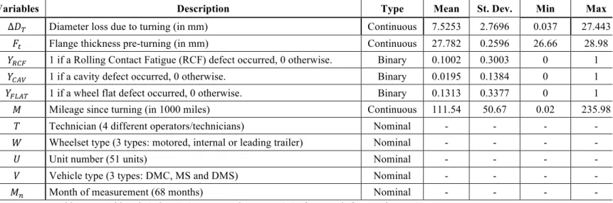
Table 1 provides the variables, their description and some statistics of the dataset collected. The dependent variable is the diameter loss due to turning (∆DQ) and the remaining variables are used as
independent/explaining variables or factors, namely: flange thickness pre-turning (𝐹'), occurrences of
Rolling Contact Fatigue (RCF), of cavities (CAV) and of wheel flats (FLAT), mileage since last turning, wheelset type (motored, internal or leading trailer), unit number (in a total of 51 units), vehicle type (in 3 types: Driving Motor Composite (DMC), Motor Second (MS), Driving Motor Second (DMS)) and the month of measurement (in a total of 68 months).
5- Applying SFA and LMM
This section starts with a brief description of the sample of turning records at the wheel lathe and then applies the SFA and LMM statistical methods described above to the sample in order to assess the technical efficiencies of the wheel lathe operators.
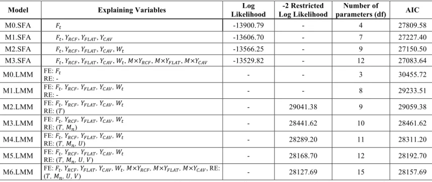
Several model specifications were run to provide a basis for comparison between SFA and LMM models: 4 model specifications for SFA (M0.SFA-∆𝐷) up to M3.SFA-∆𝐷)) and 7 model specifications for LMM
(M0.LMM-∆𝐷) up to M6.LMM-∆𝐷)). For the SFA, each model specification sequentially adds more
explaining variables, i.e. first model only considers the flange thickness (𝐹'), the second model adds the
fourth model adds some interaction terms with mileage since turning and damage defects (𝑀×𝑌TUV,
𝑀×𝑌VWX), 𝑀×𝑌UXY). Similarly, for the LMMs each specification sequentially adds fixed effects and random
effects, i.e. the first model also only considers the flange thickness (𝐹') as a fixed effect, the second model
adds the occurrence of wheel tread damage and the wheelset type (𝑌TUV, 𝑌VWX), 𝑌UXY, 𝑊') as fixed effects,
the third model adds the technician (𝑇) as a random effect, the fourth model adds the month of measurement (𝑀^) as a random effect, the fifth model adds the unit (𝑈) as a random effect, the sixth
model adds the vehicle (𝑉) as a random effect. The final seventh LMM model specification also adds the interaction terms with mileage since turning and damage defects (𝑀×𝑌TUV, 𝑀×𝑌VWX), 𝑀×𝑌UXY) for a fair
comparison with the fourth SFA model specification, i.e. so that models M3.SFA-∆𝐷) and M6.LMM-∆𝐷) have exactly the same explaining variables. Table 2 provides details on each of the estimated model and ‘goodness-of-fit’ statistics for easier comparison. Several ‘goodness-of-fit’ measures are computed for both models. The Log-likelihood value and the –2 Restricted Log-likelihood value are computed for the SFA and LMM models, respectively, and the Akaike Information Criterion (AIC) value is computed for all model specifications. The AIC is used for comparing between different SFA and LMM model specifications. It combines a goodness-of-fit measure with a measure of model complexity, i.e. the -2 Log-likelihood plus 2 times the number of parameters. AIC provides a criterion to compare different models, in which the preferred model is the one with the lowest AIC value.
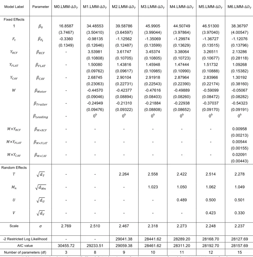
Tables 3 and 4 show the estimates for the parameters of all SFA and LMM model specifications, respectively. Regarding Table 3, all variables are statistically significant at the 5% significance level for all model specifications, except for the parameter associated with motored wheelsets (𝛽a%'%#). The flange
thickness (𝐹') has a negative effect, i.e. the lower the flange thickness, the more diameter a wheel will
lose due to turning; whereas the damage defects (𝑌TUV, 𝑌VWX), 𝑌UXY) have a positive effect, i.e. the
occurrence of tread damage increases the diameter lost due to turning. Note that the damage defects have all positive interaction terms with mileage since turning, i.e. the diameter loss required to remove tread damage increases as the mileage since turning increases. Furthermore, the scale parameters show that the term associated with inefficiency provides a higher value of variance than the term associated with random noise, i.e. 𝜎? > 𝜎; resulting into a value for 𝜆 =ccd e higher than 1. This shows that the error component associated with inefficiency (𝑢/) dominates the variability around the mean of the diameter loss due to turning, controlling for the explaining variables.
Figure 1 provides a contrast between the SFA specified in model M3.SFA-∆𝐷), an Ordinary Least Square
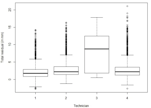
(OLS) estimation without considering inefficiency terms and a Corrected Ordinary Least Square (COLS) approach. The OLS and COLS have the same slopes, though the COLS line is shifted to the minimum diameter loss observed. A box-and-whisker plot is presented in Figure 2, for the total residual above the SFA line for different technicians based on the residuals estimated from model M3.SFA-∆𝐷). One
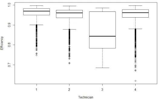
interesting finding from the statistical modelling regards the variability between wheel lathe operators. The model showed that, whilst three of the operators removed very similar amounts of material above the minimum possible (around 2.0 mm diameter on average), one operator (number ‘3’) removed significantly more (more than an average of 10.0 mm). The model is constructed to carefully control for other factors which would influence the minimum possible value to remove. For example, if operator ‘3’ was considered the most experienced and therefore given the most damaged wheels to turn. As the wheel damage types, depths, times of turning etc. were found to be similar for all operators, the analysis therefore suggests that there is an underlying difference in the turning approach adopted by operator ‘3’. This has the potential to significantly affect the overall wheelset life. Indeed the lathe operator was found to be one of the most statistically significant factors in amount of material removed at turning. Although it is beyond the scope of this paper, it would be interesting to investigate whether wheels turned by Operator ‘3’ subsequently had shorter or longer intervals to next turning. It may be that removing more material is more effective in ensuring that RCF damage is fully removed preventing early recurrence. Alternatively it may be that operator ‘3’ removed more material than necessary shortening the wheels life. In microeconomics literature, it is also common to represent the same box-and-whisker plot for different agents/firms but measuring technical efficiency (i.e. 𝑒g?h). Figure 3 represents the technical efficiency of the different wheel lathe operators. All the LMM models shown in Table 4 exhibited statistically significant estimates at the 5% significance level, except for the parameter associated with motored wheelsets (𝛽a%'%#) for the model M6.LMM-∆𝐷).
The factor associated with different technicians (𝑇) was the random effect that showed the greatest variability, followed by the random effects associated with month of measurement (𝑀^), unit (𝑈) and
vehicle (𝑉).
Finally, comparing model M6.LMM-∆𝐷) with model M3.SFA-∆𝐷), the best SFA model has a lower AIC
value (27083.64), than the best LMM models with an AIC of 28157.69. This indicates that the SFA model performed better than the LMM model. The finding suggests that using an error component structure
associated with inefficiencies, by mathematically adding a one-sided distribution, may considerably enhance the statistical models, even when comparing with a complex statistical model like the LMM. 6- Conclusions and further research This paper provided evidence of the importance of modelling the performance of different wheel lathe operators in the maintenance of railway wheelsets. By applying an SFA model, we were able to identify the technical efficiency of each wheel lathe operator, when compared to a ‘best practice’ frontier, and thus, isolate the bias due to inefficiencies of each operator, while controlling for other factors that contribute to explain the variability of the diameter loss due to turning. It also highlights the need to provide lathe operators with clear guidance and training so that they understand the effect of their decisions on wheel life. Therefore, current maintenance managers should apply this technique to identify maintenance operators, which might be able to improve their performance, and recommend them specific training. The comparison between the SFA models and LMM models showed that the error component structure that tackles technical inefficiencies provides a significant enhancement in the AIC value. This suggests that the application of statistical techniques, such as SFA, previously applied in economic analysis can also prove useful in modelling physical phenomena. For further research, it would be interesting to add more variables describing the attitudes and experience of the different technicians, trying to answer for instance whether or not more experienced technicians perform better than others. Moreover, it would also be useful to conduct further analysis on whether turning more material off might be beneficial in preventing the re-occurrence of RCF damage and cavities. In that sense, we recommend an extension of the assessment of technicians’ performance, which would necessarily imply collecting other sources of data (not available in our sample), more usual in research areas like human-computer interaction, human factors and usability engineering. Finally, we believe that the combination of mixed factors with SFA models through a hierarchical Bayesian model might provide even better results, but this is a step for the future, in which a good starting point is Griffin and Steel17, which could be combined with a previous work18. Acknowledgments The work reported in this paper was undertaken under the Strategic Partnership between the University of Huddersfield and RSSB. The authors also gratefully acknowledge the technical support provided by
industry colleagues, by Adam Bevan and Paul Molyneux-Berry at the Institute of Railway Research and by two anonymous reviewers. References 1. Bogetoft P and Otto L. Benchmarking with Dea, Sfa, and R. Springer Science & Business Media, 2010. 2. Andrade AR and Stow J. Statistical Modelling of Wear and Damage Trajectories of Railway Wheelsets. Quality and Reliability Engineering International. 2016. 3. Farrell MJ. The measurement of productive efficiency. Journal of the Royal Statistical Society Series A (General). 1957; 120: 253-90. 4. Kumbhakar SC and Lovell CK. Stochastic frontier analysis. Cambridge University Press, 2003. 5. Meeusen W and Van den Broeck J. Efficiency estimation from Cobb-Douglas production functions with composed error. International economic review. 1977: 435-44. 6. Aigner D, Lovell CK and Schmidt P. Formulation and estimation of stochastic frontier production function models. journal of Econometrics. 1977; 6: 21-37. 7. Battese GE and Corra GS. Estimation of a production frontier model: with application to the pastoral zone of Eastern Australia. Australian journal of agricultural economics. 1977; 21: 169-79. 8. Michaelides PG, Belegri-Roboli A, Karlaftis M and Marinos T. International air transportation carriers: evidence from SFA and DEA technical efficiency results (1991-2000). EJTIR. 2009; 4. 9. Scotti D, Malighetti P, Martini G and Volta N. The impact of airport competition on technical efficiency: A stochastic frontier analysis applied to Italian airport. Journal of Air Transport Management. 2012; 22: 9-15. 10. Welde M and Odeck J. The efficiency of Norwegian road toll companies. Utilities Policy. 2011; 19: 162-71. 11. Filippini M, Koller M and Masiero G. Competitive tendering versus performance-based negotiation in Swiss public transport. Transportation Research Part A: Policy and Practice. 2015; 82: 158-68. 12. Smith AS. The application of stochastic frontier panel models in economic regulation: Experience from the European rail sector. Transportation Research Part E: Logistics and Transportation Review. 2012; 48: 503-15. 13. Farsi M, Filippini M and Greene W. Efficiency measurement in network industries: application to the Swiss railway companies. Journal of Regulatory Economics. 2005; 28: 69-90. 14. Simões P and Marques RC. On the economic performance of the waste sector. A literature review. Journal of environmental management. 2012; 106: 40-7. 15. Team RC. R: A language and environment for statistical computing. Vienna, Austria: R Foundation for Statistical Computing; 2014. 2014. 16. Bates D, Maechler M, Bolker B and Walker S. lme4: Linear mixed-effects models using Eigen and S4. R package version. 2014; 1. 17. Griffin JE and Steel MF. Bayesian stochastic frontier analysis using WinBUGS. Journal of Productivity Analysis. 2007; 27: 163-76. 18. Andrade AR and Teixeira PF. Statistical modelling of railway track geometry degradation using hierarchical Bayesian models. Reliability Engineering & System Safety. 2015; 142: 169-83.
Figure 1 - Comparison between OLS, COLS and SFA approaches.
Figure 2 – Box-and-whisker4 plot for the total residual (i.e. 𝒗𝒊− 𝒖𝒊) (in mm) for different wheel lathe operators/technicians.
4 The box-and-whisker is a typical plot in statistics that helps to show the variability of a given sample. The box refers
Figure 3 - Technical Efficiency (i.e. 𝒆g𝒖𝒊) for different wheel lathe operators/technicians.
Q2). The whiskers go from the lower limit (Q1-1.5×IQR) to the upper limit (Q3+1.5×IQR), in which IQR is the interquartile range, i.e. the difference between Q3 and Q1 (IQR=Q3-Q1). The observations that go outside the whiskers range are considered outliers and are identified as simple points.
Variables Description Type Mean St. Dev. Min Max
∆𝐷) Diameter loss due to turning (in mm) Continuous 7.5253 2.7696 0.037 27.443
𝐹' Flange thickness pre-turning (in mm) Continuous 27.782 0.2596 26.66 28.98
𝑌TUV 1 if a Rolling Contact Fatigue (RCF) defect occurred, 0 otherwise. Binary 0.1002 0.3003 0 1
𝑌UXY 1 if a cavity defect occurred, 0 otherwise. Binary 0.0195 0.1384 0 1
𝑌VWX) 1 if a wheel flat defect occurred, 0 otherwise. Binary 0.1313 0.3377 0 1
𝑀 Mileage since turning (in 1000 miles) Continuous 111.54 50.67 0.02 235.98
𝑇 Technician (4 different operators/technicians) Nominal - - - -
𝑊 Wheelset type (3 types: motored, internal or leading trailer) Nominal - - - -
𝑈 Unit number (51 units) Nominal - - - -
𝑉 Vehicle type (3 types: DMC, MS and DMS) Nominal - - - -
𝑀^ Month of measurement (68 months) Nominal - - - -
Table 1 – Variables, their description, type and some statistics for a total of 6,246 observations.
Model Explaining Variables Log Likelihood -2 Restricted Log Likelihood Number of parameters (df) AIC M0.SFA 𝐹' -13900.79 - 4 27809.58
M1.SFA 𝐹', 𝑌TUV, 𝑌VWX), 𝑌UXY -13606.70 - 7 27227.40
M2.SFA 𝐹', 𝑌TUV, 𝑌VWX), 𝑌UXY, 𝑊' -13566.25 - 9 27150.50
M3.SFA 𝐹', 𝑌TUV, 𝑌VWX), 𝑌UXY, 𝑊', 𝑀×𝑌TUV, 𝑀×𝑌VWX), 𝑀×𝑌UXY -13529.82 - 12 27083.64
M0.LMM FE: 𝐹' RE: - - - 3 30455.72
M1.LMM FE: 𝐹', 𝑌TUV, 𝑌VWX), 𝑌UXY, 𝑊'
RE: - - - 8 29233.51
M2.LMM FE: 𝐹', 𝑌TUV, 𝑌VWX), 𝑌UXY, 𝑊'
RE: (𝑇) - 29041.38 9 29059.38
M3.LMM FE: 𝐹', 𝑌TUV, 𝑌VWX), 𝑌UXY, 𝑊'
RE: (𝑇, 𝑀^) - 28441.62 10 28461.62
M4.LMM FE: 𝐹', 𝑌TUV, 𝑌VWX), 𝑌UXY, 𝑊'
RE: (𝑇, 𝑀^, 𝑈) - 28289.20 11 28311.20
M5.LMM FE: 𝐹', 𝑌TUV, 𝑌VWX), 𝑌UXY, 𝑊'
RE: (𝑇, 𝑀^, 𝑈, 𝑉) - 28168.70 12 28192.70
M6.LMM FE: 𝐹', 𝑌TUV, 𝑌VWX), 𝑌UXY, 𝑊', 𝑀×𝑌TUV, 𝑀×𝑌VWX), 𝑀×𝑌UXY, RE:
(𝑇, 𝑀^, 𝑈, 𝑉) - 28127.69 15 28157.69
Table 2 – Explaining variables and comparison of the fit statistics from different models estimated for the dependent variable
diameter loss due to turning (∆𝑫𝑻). Note 1: All models included an intercept constant value (𝛃𝟎). Note 2: For the LMM
models, the Fixed Effects (FE) are presented first and the Random Effects (RE) are included in parenthesis.
Model Label Parameter M0.SFA-∆𝐷) M1.SFA-∆𝐷) M2.SFA-∆𝐷) M3.SFA-∆𝐷) 1 𝛽o 54.425 57.797 55.441 52.290 (2.3554) (2.4344) (2.5211) (2.0379) 𝐹' 𝛽Vp -1.794 -1.920 -1.829 -1.714 (0.0850) (0.0879) (0.0910) (0.0738) 𝑌TUV 𝛽TUV - 1.613 1.604 0.530 (0.0740) (0.0755) (0.2726) 𝑌VWX) 𝛽qrs' - 1.146 1.100 0.698 (0.0718) (0.0741) (0.1251) 𝑌UXY 𝛽ts; - 1.452 1.495 0.684 (0.1720) (0.165) (0.3228) 𝑊' 𝛽a%'%# - - -0.036 -0.059 (0.0631) (0.0736) 𝛽)#s/r$# - - -0.447 -0.462 (0.0693) (0.0812) 𝛽W$su/^v - - 0b 0b 𝑀×𝑌TUV 𝛽a×TUV - - - 0.009 (0.0021) 𝑀×𝑌VWX) 𝛽a×VWX) - - - 0.006 (0.0015) 𝑀×𝑌UXY 𝛽a×UXY - - - 0.013 (0.0037) Scale 𝜎; 0.5921 0.6881 0.6923 0.6884 𝜎? 4.0172 3.7159 3.6828 3.6610 𝜆 6.784 5.400 5.319 5.318 (0.2619) (0.2030) (0.2084) (0.1697) Log Likelihood -13900.79 -13606.70 -13566.25 -13529.82 AIC 27809.58 27227.40 27150.50 27083.64 Number of parameters (df) 4 7 9 12 Table 3– Estimates for the parameters of different models M0.SFA-M3.SFA for the dependent variable diameter loss due to turning (∆𝑫𝑻).
Model Label Parameter M0.LMM-∆𝐷) M1.LMM-∆𝐷) M2.LMM-∆𝐷) M3.LMM-∆𝐷) M4.LMM-∆𝐷) M5.LMM-∆𝐷) M6.LMM-∆𝐷) Fixed Effects 1 𝛽o 16.8587 34.48553 39.58786 45.9905 44.50749 46.51300 38.36797 (3.7467) (3.50410) (3.64597) (3.99044) (3.97864) (3.97040) (4.00547) 𝐹' 𝛽Vp -0.3360 -0.98135 -1.12562 -1.35069 -1.29974 -1.36727 -1.12076 (0.1349) (0.12646) (0.12487) (0.13599) (0.13629) (0.13515) (0.13796) 𝑌TUV 𝛽TUV - 3.53981 3.61747 3.45374 3.38064 3.26511 2.13286 (0.10808) (0.10705) (0.10805) (0.10723) (0.10677) (0.28118) 𝑌VWX) 𝛽VWX) - 1.50080 1.43816 1.45948 1.47444 1.51732 1.09268 (0.09762) (0.09617) (0.10985) (0.10990) (0.10888) (0.15382) 𝑌UXY 𝛽UXY - 2.68745 2.90104 2.91918 2.87964 2.83966 1.30192 (0.23063) (0.22731) (0.22543) (0.22390) (0.22174) (0.38160) 𝑊 𝛽a%'%# - -0.44570 -0.42377 -0.47616 -0.49889 -0.59099 -0.05067 (0.09046) (0.08894) (0.08403) (0.08260) (0.08472) (0.08282) 𝛽)#s/r$# - -0.24949 -0.21310 -0.21884 -0.22938 -0.37037 -0.54323 (0.09476) (0.09322) (0.08808) (0.08652) (0.09170) (0.09191) 𝛽W$su/^v - 0b 0b 0b 0b 0b 0b 𝑀×𝑌TUV 𝛽𝑀×𝑅𝐶𝐹 - - - 0.00958 (0.00213) 𝑀×𝑌VWX) 𝛽𝑀×𝐹𝐿𝐴𝑇 - - - 0.00544 (0.00155) 𝑀×𝑌UXY 𝛽𝑀×𝐶𝐴𝑉 - - - 0.02091 (0.00443) Random Effects 𝑇 𝑑) - - 2.264 2.558 2.422 2.514 2.278 𝑀^ 𝑑a^ - - - 1.023 1.050 1.062 1.049 𝑈 𝑑| - - - - 0.489 0.500 0.501 𝑉 𝑑Y - - - 0.423 0.330 Scale 𝜎 2.769 2.510 2.467 2.318 2.273 2.248 2.237
-2 Restricted Log Likelihood - - 29041.38 28441.62 28289.20 28168.70 28127.69
AIC value 30455.72 29233.51 29059.38 28461.62 28311.20 28192.70 28157.69
Number of parameters (df) 3 8 9 10 11 12 15
Table 4 – Restricted Maximum Likelihood (REML) estimates for the parameters of models M0.LMM-M6.LMM for the
dependent variable Diameter loss due to turning (∆𝑫𝑻).
a Approximate Standard Errors for Fixed Effects are included in parentheses. b This parameter is redundant.