Program and aspect metrics for MATLAB : design and implementation

(1)

Paulo Alexandre da Silva Lopes

Program and Aspect Metrics for MATLAB Design and Implementation

Tese de Mestrado

Mestrado em Informática

Trabalho efectuado sob a orientação de

Prof. Dr. João Saraiva e Prof. Dr. João M. P. Cardoso

(2)

(3)

Acknowledgements

First, I would like to thank my supervisors PhD João Saraiva and PhD João Cardoso, for the great support, helping me every time I needed.

I thank to my parents Manuel and Rosa, and all my family that have been following me in all the stages of my life, and supporting me all the time.

To my friends who always were there for me in the good and bad moments, remember-ing me that there is no impossibles. I thank also to my colleagues and friends of the Judo team of Universidade do Minho, that in all this years helped me to get great times and with whom I learned so much.

I would like to thank Susana for her support for all these years where was an important pillar in my live, and always helped me reach my goals.

Finally, I would like to thank the AMADEUS project (PTDC/EIA/70271/2006), about Aspects and Compiler Optimizations for MATLAB System Development, under FCT for funding and supporting this research.

(4)

(5)

Resumo

MATLAB é uma linguagem de programação suportada por um software interactivo de alta performance voltado para o cálculo numérico. O MATLAB integra análise numérica, cálculo com matrizes, processamento de sinais e construção de gráficos num ambiente in-tuitivo, onde as operações sobre matrizes são mais simples usando MATLAB , ao contrário do que acontece na programação tradicional.

Na linguagem MATLAB o elemento básico de informação são matrizes em que o dimen-sionamento pode ser feito dinamicamente. Este sistema permite a resolução de muitos problemas numéricos em apenas uma fracção do tempo que se gastaria para escrever um programa semelhante usando outra linguagem como o Fortran, Basic ou C 1. Além disso, as soluções dos problemas são expressas em MATLAB de forma muito semelhante à sua escrita matemática.

Por todas as suas vantagens, MATLAB tem vindo a ser uma das linguagens de progra-mação mais usadas na comunidade ciêntifica, e para atestar isso está o vasto número de livros e publicações dedicadas a esta linguagem de programação.

Os objectivos deste projecto são dois: o primeiro é desenvolver um catálogo de métricas de programas para a linguagem de programação MATLAB que irá servir para definir padrões de qualidade para programas escritos em MATLAB. O segundo é desenvolver um catálogo de métricas para aspectos, que irão ser usadas em conjunto com as métricas para progra-mas, de modo a analisar os prós e contras do uso de aspectos num programa MATLAB e perceber as vantagens na sua utilização.

Para isto a ferramenta Weaver desenvolvida anteriormente para o projecto AMADEUS, irá ser usada, uma vez que permite, durante o seu processo de ’weaving’, a análise do pro-grama MATLAB sem aspectos, a análise do aspecto envolvido neste processo, e a análise do programa MATLAB , final produzido pelo Weaver, que é o programa MATLAB origi-nal com aspectos no seu código.

1_{http://www.mathworks.com/products/matlab/}

(6)

(7)

Abstract

MATLAB is an programming language supported by an interactive software for high per-formance dedicated to the numerical calculation. MATLAB integrates numerical analysis, matrix computation, signal processing and construction of charts an friendly-use environ-ment, where operations on matrices are simplified by using MATLAB , contrary to what happens in traditional programming.

In MATLAB language the basic element of information are matrices in which the dimen-sioning can be done dynamically. This system allows the resolution of many numerical problems in a fraction of the time it takes to write a similar program in Fortran, Basic or C2. Furthermore, the solutions for problems are expressed in MATLAB much like its writ-ing in the mathematic way.

For all its advantages, MATLAB has been one of the most widely used programming languages in the scientific community, and to attest it is the vast number of books and pub-lications dedicated to this programming language. [8]

This MSc thesis’s goal is twofold: first, we wont to develop a catalog of program metrics for the programming language MATLAB, which will be used to asses the quality of pro-grams in MATLAB. Second, we wont develop a catalog of aspect metrics, that will be used with the program metrics in order to analyze the pros and cons of the use of aspects an a MATLAB program, so as to realize if there is some advantage in its use.

For this the Weaver tool developed in previous work in the context of AMADEUS project will be used, once this process allow analyze MATLAB programs without aspects, analyze the aspect involved in the weaver process, and analyze the resulting MATLAB program of this process, which is the original MATLAB program with aspects embedded on its code.

2_{http://www.mathworks.com/products/matlab/}

(8)

(9)

List of Figures

1.1 Sum of a Matrix on MATLAB Language . . . 4

1.2 Sumvals function in MATLAB . . . 6

2.1 Control flow graph of the function ’sumvals’ . . . 16

2.2 Matrix Multiplication on MATLAB . . . 20

2.3 Matrix Multiplication on C . . . 20

3.1 MATLAB analysis process . . . 30

3.2 Sumvals function with logging . . . 32

3.3 ’Sumvals’ function without concerns . . . 33

3.4 LOC values of the original MATLAB and the AO version . . . 38

3.5 Number of operators of the original MATLAB and the AO version . . . 39

3.6 Number of operands of the original MATLAB and the AO version . . . 40

3.7 Vocabulary vales of the original MATLAB and the AO version . . . 41

3.8 Program Length values of the original MATLAB and the AO version . . . 42

3.9 Calculated Program Length values of the original MATLAB and the AO version . . . 43

3.10 Volume values of the original MATLAB and the AO version . . . 44

3.11 Difficultyvalues of the original MATLAB and the AO version . . . 45

3.12 Effort values of the original MATLAB and the AO version . . . 46

3.13 Graphic of cyclomatic complexity values . . . 47

4.1 MATLAB analysis process . . . 50 ix

(12)

4.2 AST of ’sumvals’program . . . 51

4.3 CFG of ’sumvals’ function . . . 52

4.4 MATLAB ’weaved’ analysis process . . . 54

4.5 Example of Betweenness Centrality calculation . . . 58

4.6 Example of For loop for Betweenness Centrality Values . . . 59

4.8 Example of For loop for Page Rank Values . . . 60

4.7 Example of Page Rank calculation . . . 61

4.9 Loops to obtain the number of edges and the number of nodes . . . 62

(13)

List of Tables

2.1 Metrics results . . . 19

2.2 Average packages values . . . 22

2.3 Intervals of quality . . . 22

2.4 ’sumvals’ results . . . 23

2.5 classification of the measurements of the programs . . . 24

2.6 Classification of the programs . . . 25

3.1 Aspect metrics results . . . 34

3.2 Metrics results on Aspects . . . 35

3.3 Metrics results of programs without Concerns . . . 36

3.4 Sum of the Tab. 3.2 and Tab. 3.3 (AO version) . . . 37

4.1 Final results . . . 53

(14)

(15)

Chapter 1 Introduction

MATLAB is a popular dynamic programming language used for scientific and numerical programming with a very large and increasing user base. Data from MathWorks shows that the number of users of MATLAB was 1 million in 2004, with the number of users doubling every 1.5 to 2 years. 1

Certainly it is one of the key languages used in education, research and development for scientific and engineering applications. There are currently over 1200 books based on MATLAB and its companion software, Simulink 2_{. This large and diverse collection of}

books illustrates the many scientific areas which rely on computational approaches and use MATLAB.

The key features of MATLAB includes no need to declare variables (floating-point, double precision representation is the default data type), operator overloading, function polymorphism and dynamic type specialization. However, tasks such as exploiting non-uniform fixed-point representations, monitoring certain variables during a timing window, or including handlers to watch specific behaviors are extremely cumbersome, error-prone and tedious. Each time these features are necessary, invasive changes on the original code, as well as insertion of new code need to be performed. This problem is felt in other imple-mentation issues as well, since MATLAB can be regarded as a specification rather than an implementation language. Other open issues are related to efficient automatic synthesis of MATLAB specifications to a software language or a hardware description language. The AMADEUS project addresses the enrichment of MATLAB with aspect-oriented

ex-1_{www.mathworks.com}_{/company/newsletters/news_notes/clevescorner/jan06.pdf}

2_{http://www.mathworks.com/support/books}

(16)

tensions [19, 29] to include additional information (e.g., type and shape of variables) and experiment different implementations features (e.g., different implementations for the same function, certain type binding for variables, etc.). The proposed aspects aim to configure the low-level data representation of real variables and expressions, to specifically-tailored data representations that benefit from a more efficient support by target computing engines (e.g., fixed-point instead of floating-point representation). The project approach also aims to help developers to introduce handlers (code triggered when certain conditions may occur and with a richer functionality than assertions) and monitoring features, and to configure functions implementations. We believe aspect-oriented extensions will help system mod-eling simulation, and exploration of features conceiving system implementation. One of the advantages is related to the fact that a single version of the specification can be used throughout the entire development cycle rather than maintaining multiple versions, as it currently the case.

MATLAB is a widely used language, and thus, there is a large number of (legacy) pro-grams developed in MATLAB . The goal of this MSc project is to build on previous work developed in the AMADEUS project that aimed at providing an AOP extension to MAT-LAB. In [8], a preliminary version of the Aspect-MATLAB language was proposed by the members of the project. This extension models aspects as a set of (aspect) rules while maintaining the original program unchanged. In this project we will define a catalog of metrics for MATLAB and a catalog of metrics for aspects. These catalogs will serve two purposes: firstly we will use the metrics to asses the quality of MATLAB programs. Secondly we use these two catalog of metrics to compare MATLAB program with the equivalent Aspect-Oriented version of it.

This thesis was developed in the context of the AMADEUS project, a FCT funded project (PTDC/EIA/70271/2006).

Part of this work was funded by AMADEUS under a BI grant.

1.1 The MATLAB Programming Language

“MATLAB is a high-level language and interactive environment that enables you to perform computationally intensive tasks faster than with traditional

(17)

pro-1.1. THE MATLAB PROGRAMMING LANGUAGE 3 gramming languages such as C, C# and Fortran.”in3

In this section we introduce the MATLAB language and its programming environment, as well as some exclusive features and programming particularities when developing pro-grams in MATLAB.

1.1.1 Introduction to MATLAB

MATLAB is a high-performance language for technical computing. It integrates compu-tation, visualization, and programming in an easy-to-use environment where problems and solutions are expressed in familiar mathematical notation. Typical uses include :

• Math and computation; • Algorithm development;

• Modeling, simulation and prototyping; • Data analysis, exploration and visualization; • Scientific and engineering graphics;

• Application development, including Graphical User Interface building;

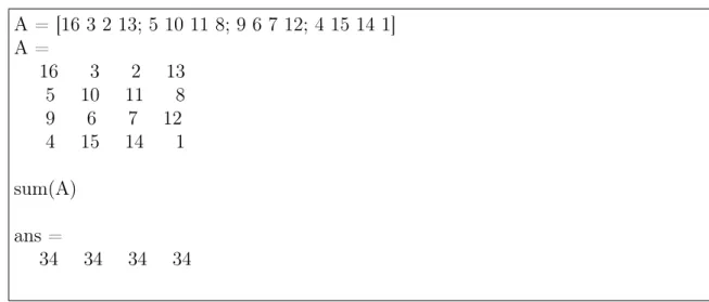
MATLAB is a programming language supported by an interactive software, whose ba-sic data element are arrays whose dimensioning is done dynamically. This allows us so solve many technical computing problems, specially those with matrix and vector formu-lations, in a fraction of the time it would take to write a program in a scalar non interactive language such as C or Fortran. An example of a matrix operation is the sum of a matrix that is very simple to write in MATLAB language, FIG. 1.1.

In fact, the name MATLAB stands for matrix laboratory. It was originally written to provide easy access to matrix software developed by the LINPACK and EISPACK projects, which together represent the most of the state-of-art in software for matrix com-putation.

(18)

A = [16 3 2 13; 5 10 11 8; 9 6 7 12; 4 15 14 1] A = 16 3 2 13 5 10 11 8 9 6 7 12 4 15 14 1 sum(A) ans = 34 34 34 34

Figure 1.1: Sum of a Matrix on MATLAB Language

The MATLAB system consists of five main parts: The MATLAB language

This is a high-level matrix/array language with control flow statements, functions, data structures, input/output, and object-oriented programming features. It allow both "programming in the small" to rapidly create quick and dirty throw-away pro-grams, and "programming in the large" to create complete large and complex appli-cation programs.

The MATLAB working environment

This is the set of tools and facilities that we work with as the MATLAB user or programmer. It includes facilities for managing the variables in our workspace and importing and exporting data. It also includes tools for developing, managing, de-bugging, and profiling M-files, which are MATLAB functions files, the MATLAB’s applications.

Handle Graphs

This is the MATLAB graphics system. It includes high-level commands for two-dimensional and three-two-dimensional data visualization, image processing, animation, and presentation graphics. It also includes low - level commands that allow you to fully customize the appearance of graphics as well as to build complete Graphical User Interfaces on our MATLAB applications.

(19)

1.1. THE MATLAB PROGRAMMING LANGUAGE 5 The MATLAB mathematical function library

This is a vast collection of computational algorithms ranging from elementary func-tions like sum, sine, cosine, and complex arithmetic, to more sophisticated funcfunc-tions like matrix inverse, matrix eigenvalues, Bessel functions, and fast Fourier transforms. The MATLAB application Program Interface (API)

This is a library that allows programmers to write C and Fortran programs that in-teract with MATLAB . It include facilities for calling routines from MATLAB (dy-namic linking), calling MATLAB as a computational engine, and for reading and writing M-files.

MATLAB has evolved over a period of years with input from many users. In university environments, it is a widely adopted language/tool for introductory and advanced courses in mathematics, engineering and science. In industry, MATLAB is the tool of choice for high-productivity research, development and analyze.

It features a family of applications-specific solutions called toolboxes. Very important to most users of MATLAB, toolboxes allow us to learn and apply specialized technol-ogy. Toolboxes are comprehensive collections of MATLAB functions (M-files) that ex-tend the MATLAB environment to solve particular classes of problems. Areas in which toolboxes are available include signal processing, control system, neural networks, fuzzy logic, wavelets, simulation and many others.

MATLAB supports Object Oriented Programming (OOP), which introduce the concepts of class, object and inheritance, but apart from architecture and designing, there is no use-ful new advantages to code control or debugging, which still implies direct changes in the source code. Garbage collection is not supported, first because of the complexity associ-ated with managing objects lifecycles and lastly because it makes testing and debugging an application more difficult. For instance, one can stop the workspace and see all the activi-ties that took place, while a garbage collection engine could destroy steps that can not be repeated.

There are more than 1200 books that, alone, prove the wide usage of MATLAB and associated functions and tools.

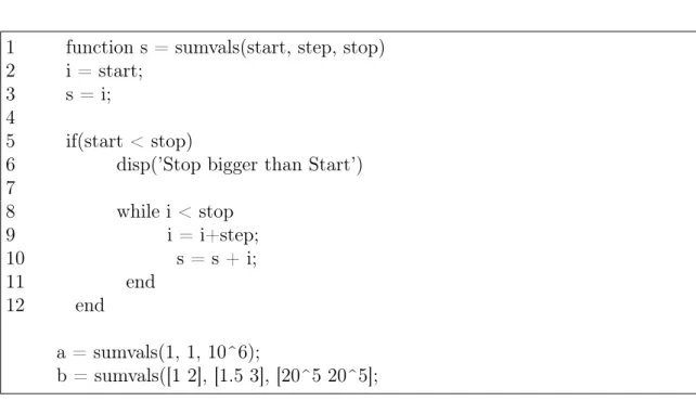
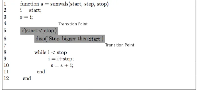
In MATLAB the definition of functions is very similar to C. In Fig. 1.2, we present the MATLAB function with name ’sumvals’ taken from [9]:

(20)

1 function s = sumvals(start, step, stop) 2 i = start;

3 s = i;

4

5 if(start < stop)

6 disp(’Stop bigger than Start’) 7 8 while i < stop 9 i = i+step; 10 s = s + i; 11 end 12 end a = sumvals(1, 1, 10^6); b = sumvals([1 2], [1.5 3], [20^5 20^5];

Figure 1.2: Sumvals function in MATLAB

The function ’sumvals’ is designed to sum numbers within a range of values. There are a few differences from MATLAB to C functions. First, the variable returned by the func-tion (in this case is ’s’), is declared in the funcfunc-tion definifunc-tion, instead of having a special primitive to do this, like the ’return’ in C. In fact, MATLAB functions may return more than one variable.

This function will be used to show how the metrics works, as we will see in chapter 2.

1.2 Metrics

“Measurement is the process by which number or symbol are assigned to at-tributes of entities in the real world in such a way as to describe them according to clearly defined rules”. [14]

Why metrics are so important to us? The answer is very simple, it is because they make possible understand our world, everything that surrounds us, man has the need of control-ling every single entity [14], and does that by measuring.

(21)

1.2. METRICS 7 Measurement is not solely the domain of professional technologists, each of us uses it in everyday life. Price acts as a measure of a value of an item in a shop, and we calculate the total bill to make sure the shopkeeper gives us correct change. We use height and size measurements to ensure that our clothing will fit properly. So measurement help us to un-derstand our world, interact our surroundings and improve our lives.

Measurement captures information about attributes of entities. An entity is an object such as a person or a room or even a journey or the testing phase of a program code.

We want to describe the entity by identifying characteristics that are important to us in distinguishing one entity from another. An attribute is a feature or property of an entity. Typical attributes include the area or color (of a room), the cost (of a journey) or the quality of a source code of a program.

When we describe entities by using attributes we often define the attributes using numbers or symbols. Thus, price is designated as a number of euros, while height is defined in terms of centimeters (or inches).

Measurement is a process whose definition is far from clear-cut. Many different authori-tative views lead to different interpretations about what constitutes measurement. To un-derstand what measure is, we must ask a host of questions that are difficult to answer. For example:

The height of a person is a commonly understood attribute that can be measured, but what about others attributes of people, such as intelligence?

Is intelligence adequately measured by as IQ test score? Similarly, wine can be measured in terms of alcohol content ("proof"), but wine quality be measured using the ratings of experts?

The accuracy of a measure depends on the measuring instrument as well as on the defi-nition of the measurement. For example, length can be measured accurately as long as the ruler is accurate and used properly. But some measures are not likely to be accurate, either because the measurement is imprecise or because it depends on the judgment of a human intelligence.

In software the measurement is an essential element of management, there is a little chance of controlling what we cannot measure.

(22)

“You can’t manage what you can’t control, and you can’t control what you don’t measure.” [11].

Software metrics are measures of some property of a piece of software namely, its source code or its specification. There are a several aspects of measuring software at-tributes, like specification related measures (e.g. function point metrics), process metrics (e.g. average time spent for fixing a bug) or product metrics.

Although the fundamental assumption of software quality assurance states that the quality of a software is in strict correlation with the quality of the process which was used during the development phase, product metrics have their reason of existence because of the fol-lowings:

• It is often the case that a version of the system already exists when a process based quality assurance is introduced (nothing is known about the quality of the already existing program).

• Product metrics validate process metrics.

• A prototype product is already available at early stages of the development, therefore product metrics and other product related attributes can be calculated.

Therefore, a well constructed software quality assurance methodology has to utilize both process and product related metrics to complement each other.

Over the years the measurement in software has proved to be the rule that every devel-oper should follow. The software metrics help to avoid pitfalls as a cost overruns, i.e., most projects fail to separate design and coding costs. Doing so helps identifying where problem exist, other problem that the software metrics help to resolve is clarify goals, in the projects goals are often fuzzy, and so it is difficult to quantify how well they have been achieved. Metrics can help answering many questions like, for example:

(23)

1.3. CONTRIBUTIONS 9 • How productive is the staff?

• How good is the code being developed?

• How can the code under development be improved?

The notion of software metrics is used every day by programmers, for example, it is known for all programming languages that a function with too many arguments or too many lines of code is difficult to understand and to update/maintain. Indeed, software pro-grammers use an empirical notion of metrics to improve their programs.

In conclusion we can perfectly say that software metrics play a crucial role in the con-tinuos refactoring approach of software maintenance. The role of metrics in software is an active area of research, as can be seen in the annual international workshop on Quantitative Aspect of Programming .4

1.3 Contributions

1.3.1 Aspect - MATLAB

There are some works that, in context of Aspect Oriented approach for MATLAB, con-tributes for the development of this kind of paradigm.

To the best of our knowledge the work propose in [8] was the first approach considering aspect oriented programming extensions for MATLAB. This work suggests various useful AOP features, specially those to specify different numeric data types. It has also pointed out the importance of AOP for MATLAB and suggest some further use cases.

Others approaches like [3] took [8] as inspiration, and implemented an aspect-oriented language for MATLAB. They create a language that allow implement typically AOP use cases, such as performance profiling and data annotations, on MATLAB programs.

A work developed for the AMADEUS project [21] also presents a language to add aspect oriented mechanisms to MATLAB, this language was then used to develop a Weaver, [20], that automates this process of adding aspects to MATLAB programs.

(24)

1.3.2 Software Metrics

Software metrics have a long history, since the very beginning of the software industry, companies were already concerned with the quality of their product and (mainly) with their coast. So although the first dedicated book on software metrics was not published until 1976 [16], the history of active software metrics dates back to the late-1960’s. In that early times, the Lines of Code measure (LOC or KLOC for thousands of lines of code) was used routinely as the basis for measuring both programmer productivity (LOC per programmer month) and program quality (defects per KLOC). In other words LOC was being used as a surrogate measure of different notions of program size. The early resource prediction models (such as those of [27] and [5]) also used LOC or related metrics like delivered source instructions as the key size variable. In 1971 Akiyama [32] published what we believe was the first attempt to use metrics for software quality prediction when he proposed a crude regression-based model for module defect density (number of defects per KLOC) in terms of the module size measured in KLOC. In other words he was using KLOC as a surrogate measure for program complexity.

The need for more discriminating measures became especially urgent with the increas-ing diversity of programmincreas-ing languages. Thus, the decade startincreas-ing from the mid-1970’s saw an explosion of interest in measures of software complexity (pioneered by the likes of [17] and [22]) and measures of size (such as function points pioneered by [1] and later by [31]) which were intended to be independent of programming language.

Work on extending, validating and refining complexity metrics, works like [10], has been a dominant feature of academic metrics research up to the present day [13, 34].

So due to its importance, in our days software metics are very used by the most of soft-ware companies.

1.3.3 Aspect-Oriented Metrics

Up to now, there are a lot of studies about metrics for Aspect Oriented paradigm. Lopes’ work [18] has contributed for the increasing interest in this area. She has defined a set of different metrics for separation of concerns, but the Lopes’ metrics only capture different dimensions of separation of concerns. In addition, the definition of her metrics is quite strongly coupled to her empirical study and tailored to the distribution concern in Java

(25)

1.4. ORGANIZATION 11 code.

Zhao, [33], also proposes a metrics suite for aspect-oriented software, which is specifically designed to quantifys the information flows in an aspect-oriented program . His metrics are based on a dependence model for aspect-oriented software that consists of a group of de-pendence graphs; each can be used to explicitly represent various dede-pendence relations at different levels of an aspect-oriented program. But the use of such metrics requires that software engineers construct a number of dependence graphs for different levels of modu-larity, such as the method dependence graph, the advice dependence graph, the introduction dependence graph, and so on. As a consequence, such metrics are very complex to under-stand and use, and requires the implementation of a dependence analysis tool that is likely to differ from one language to another. In addition, Zhao’s metrics are not derived from well-tested metrics, and the associated dependence model is not based on any well-known software engineering model.

Other studies like [4] proposed a unified coupling framework for AOP. In order to consis-tently and unambiguously define coupling measurements, they defined new terminologies for representing components of AO systems. In their framework, they considered two AOP languages, AspectJ and CaesarJ. They have extended their framework from Briand’s frameworks [2, 6] and tried to maximize the use of the terminology and coupling criteria originally defined in Briand’s frameworks.

They have shown how the framework can be instantiated for Java, AspectJ and CaesarJ. Also they demonstrated the applicability of the framework by using it on an existing cou-pling metric.

Studies for this kind of metrics have increased over the years, and proof of this is the con-siderable amount of papers published5.

1.4 Organization

The main body of this thesis is diveded as follows:

• Chap. 2 present our metrics suite for MATLAB, and introduce some results for MAT-LAB programs examples

(26)

• Chap. 3 presents the aspects for MATLAB , by introducing the aspect language (DSAL), and our aspect metrics suite. This chapter also presents the classification of our MATLAB programs.

• Chap. 4 introduce the tools for measurement of quality of MATLAB programs. • Chap. 5, summarizes what has been achieved and what could be done next.

(27)

Chapter 2 Metrics for MATLAB

In this chapter we will present the metrics we have implemented to give us some feedback on the quality of program we are analyzing.

Our catalogue of metrics consists of 12 metrics, each one analyzes a different aspect of the program. This catalogue of MATLAB source code metrics is the building block for our MATLAB quality model that we propose to assess the quality of MATLAB software.

2.1 Metrics Suite

This suite is composed by 12 metrics. Each metric is defined and described next. We will use our running example: ’sumvals’ function, presented in Fig. 1.2, to see the results of the metrics in a real MATLAB program.

Lines of Code: this is the very first metric used in software engineering to assess the quality of source code programs (as discussed in section 1.3.2), so, this metric give us the total number of lines of code of an MATLAB program.

In the example of the ’sumvals’ function, Fig. 1.2 we have 12 lines of code, so LOC= 12.

Distinct Number of Operands: this metric gives us the number of distinct operands on 13

(28)

a MATLAB program.

In our ’sumvals’ function we have used the following operands i, start, s, stop, and step. Thus, the final result of this metric is 5 (#operands= 5).

Distinct Number of Operators : this metric gives us the number of distinct operators on an MATLAB program.

In ’sumvals’ function we have used the following operators =, <, and +. Thus, the final result of this metric is 3 (#operators= 3).

Halstead’s Complexity: this suite of metrics was developed to measure a program’s complexity directly from source code. The suite of Halstead’s measures is composed of six measures that emphasize computational complexity of a program: Program Vocabulary, Program Length, Calculated Program Length, Volume, Difficulty, and Effort. These mea-sures are simple to calculate, however, in order to automate the calculations process, strong rules for identifying the operands and operators have to be stablished [26].

Let n1, n2, N1, and N2 be the number of distinct operators, the number of distinct operands, the total number of operators, and the total number of operands. Then, the metrics that con-stitutes the Halstead suite are defined as follows:

• Program Vocabolary: n= n1 + n2 • Program Length : N = N1 + N2

• Calculated Program Length: ˆN = n1 × log2n1+ n2 × log2n2

• Volume: V = N × log2n • Difficulty: D = n1 2 × N2 n2 • Effort: E = D × V

Please note, that the Difficulty measure is related to the difficulty to write or understand a program.There is an usual way to translate the effort measure into actual running time code, and this way is done using of the following relation: [17]

(29)

2.1. METRICS SUITE 15

Time required to program(T)= E 18

The time to implement or understand a program (T) is proportional to the effort. Empirical experiments can be used for calibrating this quantity. Halstead has found that dividing the effort by 18 gives an approximation for the time in seconds.

Let us analyze this suite in our running example: The values of this measurements for the ’sumvals’ function depends of n1, n2, N1, and N2.

The n1 and n2 we already see them is 3 and 5 respectively, and the values of N1, and N2 is 18 and 9 respectively. With this values we get the Halstead’s Complexity for the function ’sumvals’;

• Program Vocabolary: n= 3 + 5 = 8 • Program Length : N= 18 + 9 = 27

• Calculated Program Length: ˆN = 3 × log23+ 5 × log25= 16.36

• Volume: V = 27 × log28= 81 • Difficulty: D = 3 2 × 18 5 = 5.4 • Effort: E = 5.4 × 81 = 437.40

but what can we say about these results? Are they good or bad? Well, having just these values we are not able to say anything, once these measures don’t have units, and this is well-known problem of the Halstead suite: there is no qualitative interpretation of the num-bers. In fact, there is no consensus in the scientific community on how to interpret Halstead results. However, this suite is widely used in a context where the results can be compared with some reference values.

So these metrics have to be used in comparison with reference values in MATLAB . In section. 2.3, we will present MATLAB reference values defining by analyzing a large MATLAB repository and we will use to assess the quality of ’sumvals’ function.

(30)

Cyclomatic Complexity: or conditional complexity, or MacCabe Complexity is used to indicate the complexity of a program. It directly measures the number of linear indepen-dent paths through a program’s source code.

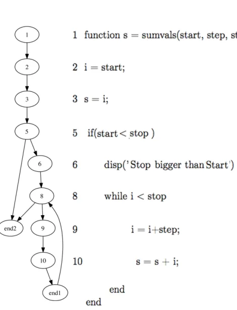
MacCabe Cyclomatic complexity is computed using the control flow graph (CFG) of the MATLAB program.

and it is calculated by the following formula: CC = E − N + p

(31)

2.1. METRICS SUITE 17 where E is the number of edges, N is the of nodes and p is the number of connected components [26]. The nodes of the graph correspond to an indivisible group of commands of a program, and, a directed edge connects two nodes if the second command might be executed immediately after the first command. The following table shows us how to inter-pret the values of this measure:

Complexity value for a program Risk thresholds

0 - 3 Simple, low risk of defects

4 - 6 Complex, moderate risk

7 - 8 Complex, possible high risk

9 and higher Consider unstable

Let us analyze the Cyclomatic Complexity of our running example. Fig. 2.1 presents the CFG of ’sumvals’ function, where we have E = 12, N = 10 and p = 1, so the Cyclomatic Complexity of this function is 11 − 10+ 1 = 2.

Centrality Measures: Like cyclomatic complexity this measure uses a CFG to be com-puted, there are various measures of the centrality of a vertex within a graph that determi-nate the relative importance of a vertex within the graph 1 _{[15], in our case we have two}

centrality measures, the Betweenness centrality and Page Rank.

• Betweenness Centrality: is a centrality measure of a vertex within a graph (there is also edge betweenness, which is not discussed here). This metric gives us the ver-tices that occur on many shortest paths between other verver-tices. These verver-tices have higher betweenness BC(v) than those that do not. Its definition is given by :

BC(v) of a vertex v ∈ V is the sum of vertices u, w ∈ V, of the fraction of shortest paths between u and w that pass through v:

BC(v)= X

u,w∈V u,v,w

ϑuw(v)

ϑuw

1_{for example, how important a person is in the social network, or in theory of space syntax, how important}

(32)

where ϑuw(V) denotes the total number of shortest path between u and w that pass

through vertex v and ϑuw denotes the total number of shortest paths between u and

w[23].

• Page Rank: 2 _{[24] is the same algorithm developed by Larry Page and used by}

google on web search, but here we use it to ranking nodes instead web pages.

Please note the Betweenness centrality and PageRank, were implemented in our tool, using an external tool called Graph-tool3, that calculates this specific measures on a graph, in this case, the CFGs of a MATLAB program, but we will give you more details in chapter 4.

2.2 Metrics for quality of MATLAB code

In this section we will show some results of applying these metrics to MATLAB programs. We use two different packages, we use the MATLAB code of a multi-criteria based applica-tion developed for site selecapplica-tion for spacecraft landing on planets [12, 25, 28], referred here as IMPACTED, and, an library package more specifically an Robotic library. This library belongs to the repository of MATLAB programs of the AMADEUS project .

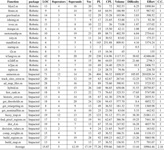
Table 2.1 presents the metrics suite for these two MATLAB applications. We include the results of 10 metrics, namely:

• LOC (column 3)

• Distinct Number of Operands (column 4) • Distinct Number of Operators (column 5) • Program Length (column 6)

• Program Vocabulary (column 7)

2_http:_{//www.smashingmagazine.com/2007/06/05/google-pagerank-what-do-we-really-know-about-it/}

(33)

2.2. METRICS FOR QUALITY OF MATLAB CODE 19 • Calculated Program Length (column 8)

• Volume (column 9) • Difficulty (column 10) • Effort (column 11)

• Cyclomatic Complexity (column 12)

Function package LOC #operators #operands Voc PL CPL Volume Difficulty Effort C.C. fdyn2.m Robotic 13 4 16 20 70 72 302.53 6.25 1890.84 2 ftrans.m Robotic 9 5 14 19 44 64.91 186.90 5.17 967.92 1 gravload.m Robotic 14 3 9 12 29 33.28 103.96 3.83 398.52 2 ishomg.m Robotic 9 2 7 9 17 21.65 53.88 1.71 92.38 2 isvec.m Robotic 13 2 8 10 22 26 73.08 1.87 137.02 3 itorque.m Robotic 4 1 6 7 15 15.50 42.11 1.08 45.61 1 motomanhp.m Robotic 10 4 19 23 89 88.71 402.59 6.84 2754.61 1 roty.m Robotic 6 2 9 11 24 30.52 83.02 2.11 175.27 1 standford.m Robotic 6 3 5 8 145 251.88 809.81 4.16 3374.24 1 startup.m Robotic 6 1 1 2 2 0 2 0.5 1 1 t2r.m Robotic 8 3 5 8 15 16.36 45 3 135 3 tr2angvec.m Robotic 42 9 20 29 230 114.96 1117.33 38.02 42486.68 3 tr2diff.m Robotic 9 6 9 15 86 44.03 335.99 21.66 2798.3 2 tr2jac.m Robotic 4 3 7 10 69 24.40 229.21 10.5 2406.73 1 trplot.m Robotic 15 3 8 11 23 28.75 79.56 3 238.70 3 uninorm.m Impacted 71 12 14 26 404 96.32 1898.97 105.85 201020.34 9 track_sites_error.m Impacted 20 7 12 19 63 62.67 267.61 12.25 3278.33 4 ad_map_files.m Impacted 28 5 16 21 89 75.60 390.91 9.53 3725.92 2 hybrid.m Impacted 18 11 15 26 140 96.65 658.06 31.53 20750.87 4 hist_rank.m Impacted 18 9 13 22 73 76.63 325.53 17.65 5747.00 1 historic_error.m Impacted 13 4 14 18 67 61.30 279.38 7.28 2035.51 1 get_thresholds.m Impacted 18 4 20 24 126 94.43 577.70 8.4 4852.72 1 get_retargeting.m Impacted 8 4 9 13 49 36.52 181.32 7.55 1369.98 1 get_nominalSite.m Impacted 9 4 6 10 25 23.50 83.04 5.33 442.92 1 fuzzy_trap.m Impacted 19 12 13 25 123 91.12 571.19 38.30 21881.13 4 find_pixel_regions.m Impacted 17 7 12 19 91 62.67 386.56 19.25 7441.30 2 dist_d.m Impacted 19 6 7 13 67 35.16 247.92 16.28 4037.70 2 decision_values.m Impacted 11 2 7 9 24 21.65 76.07 2.14 163.02 1 comp_weights.m Impacted 15 4 9 13 45 36.52 166.51 6.66 1110.13 2 build_regions.m Impacted 27 9 19 28 92 109.23 442.27 13.26 5865.98 2 build_map.m Impacted 13 4 9 13 37 36.52 136.91 5.77 791.07 3 Average 15.87 5 12.19 17.19 77.26 559.66 340.55 13.44 10964.46 2.16

(34)

Looking at the results on Tab. 2.1, the measure may cause some surprise, is the Cy-clomatic Complexity (CC) due to their low values. These results derived from the unique properties of MATLAB programming language, like matrix manipulations.

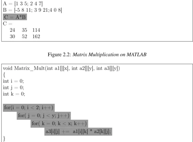
If we compare the operation of matrix multiplying in MATLAB with other programming language, C for example, we can realize the difference of complexity between them. The Fig. 2.2 and 2.3 help to illustrate this example.

A = [1 3 5; 2 4 7] B = [-5 8 11; 3 9 21;4 0 8] C = A*B C = 24 35 114 30 52 162

Figure 2.2: Matrix Multiplication on MATLAB void Matrix_Mult(int a1[][x], int a2[][y], int a3[][y])

{ int i = 0; int j = 0; int k = 0; for(i = 0; i < 2; i++) for( j = 0; j < y; j++) for( k = 0; k < x; k++)

a3[i][j] += a1[i][k] * a2[k][j]; }

Figure 2.3: Matrix Multiplication on C

As is showed in Fig. 1.1, when we calculate the matrix multiplication in MATLAB, a simple line is enough, in this case C = A ∗ B, i.e., there is no complexity (CC = 0), but to do the same operation in C, are necessary three For loops (CC= 3), that is clearly more complex than the MATLAB version. Thus, the programs are small (between 4 and 7 LOC), this example helps to illustrate why the Cyclomatic Complexity values are low.

(35)

2.2. METRICS FOR QUALITY OF MATLAB CODE 21 Looking at each package individually, we can see clear differences between a reusable MATLAB library and a MATLAB industrial application, in this case Robotic and IM-PACTEDpackages.

The results for each one of them show interesting measures, but, at the same time pre-dictable: for example, the LOC average,Tab. 2.2, is bigger in the IMPACTED programs that in Robotic. There are two possible reasons to that, first of all, it is because we are deal-ing with a library composed by functions with operations, like move, rotate, etc., to be used in robotic applications. This operations are significantly more smaller than the operations defined in the functions of an industrial application like IMPACTED.

The second one is because we are comparing MATLAB programs developed from a more generic approach, in order to allow it reuse, with MATLAB programs develop for an spe-cific goal, i.e., specialized programs. For example thinking on very simple example pro-gram like the sum of two values read from keyboard, the algorithm is something like: Read value1

Read value2

Return value1 + value2

but, if we want specialize this program to work on integers only, then the resulting algorithm is more complex:

Read value1

Test if is an Int if not

Return error message

Read value2

Test if is an Int if not

Return error message

Return value1 + value2

Furthermore if we analyze the Difficulty, Effort, and Cyclomatic Complexity values, this difference is further enhanced, so remain the idea that when we develop more specific

(36)

MATLAB programs, we take the risk of loose quality.

Package LOC #operators #operands Voc PL CPL Volume Difficulty Effort C.C.

Robotic 11.2 3.4 9.5 15.6 58.7 55.5 264.1 7.3 3692.3 1.8

Impacted 20.25 6.5 12.2 18.7 94.68 63.52 418.1 20.7 17782.1 2.5

Table 2.2: Average packages values

2.3 Quality Model for MATLAB Programs

In order to define a quality model for MATLAB we consider four different levels of "qual-ity", and we define metrics ranges for each of such intervals.

The first interval is the interval of very good values, i.e., is the interval of desirable values for any program. If a program has, for all metrics, its values in this interval, then its quality is undeniable.

The second one is the interval of good values, i.e., is the interval where most values will fit, in other words, i.e., the interval of average values, and here, the lower the better will be the quality value, once is closer to the range of very good values.

The third interval is the interval of acceptable values, i.e., are values bellow of the average of quality values, but nevertheless gives some quality to the program.

At last the interval of values without quality, i.e, any value belonging to this interval, indi-cate that for this metric, the program doesn’t has quality.

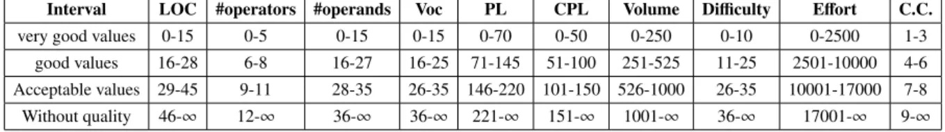
Tab. 2.3 show the intervals defined for each metric.

To define these intervals we apply our metrics in the MATLAB programs presented in this thesis and in others MATLAB programs from the AMADEUS repository. Then comparing the final results of each metric we defined the values for the intervals. In these definitions also contributed, the observation of others thresholds languages, such java or C.

Interval LOC #operators #operands Voc PL CPL Volume Difficulty Effort C.C. very good values 0-15 0-5 0-15 0-15 0-70 0-50 0-250 0-10 0-2500 1-3

good values 16-28 6-8 16-27 16-25 71-145 51-100 251-525 11-25 2501-10000 4-6 Acceptable values 29-45 9-11 28-35 26-35 146-220 101-150 526-1000 26-35 10001-17000 7-8 Without quality 46-∞ 12-∞ 36-∞ 36-∞ 221-∞ 151-∞ 1001-∞ 36-∞ 17001-∞ 9-∞

(37)

2.3. QUALITY MODEL FOR MATLAB PROGRAMS 23 Having as reference the values presented in Tab. 2.3, we can compare with the values obtained in Tab. 2.1, and then proceed to the classification of the programs analyzed. But first let’s start to classify our running example, the ’sumvals’ function, for the classification we will use the classification system by stars(?). Being that this classification goes from one star to five stars, where one star means that the program is very bad, two stars means the program is bad, three means is reasonable, four stars means is good, and five stars means is excellent.

So, comparing the values, Tab. 2.4, of ’sumvals’ function with the reference values in Tab. 2.3:

Name LOC #operators #operands Voc PL CPL Volume Difficulty Effort C.C. sumvals 12 3 5 8 27 16.36 81 5.4 437.40 1

Table 2.4: ’sumvals’ results

we can give a classification to ’sumvals’ function, and as all the values are in the interval of very good values, we give a classification of five stars (? ? ? ? ?) to this function.

We can easy classify the ’sumvals’ because we are only analyze one program, and in this case all the measurements are in the interval of optimal values.

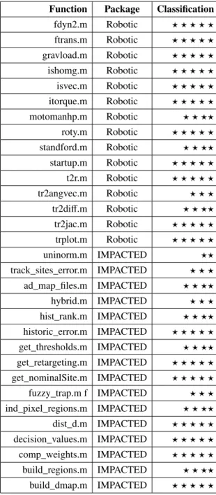
To assess the quality of the MATLAB programs presented previously, we will use this classification system to give a classification for each measure for each program, as is pre-sented by Tab. 2.5, and then we take in this classification and make an average for each program. This average will be the final classification of the programs, Tab. 2.6 present this final classification.

(38)

Function LOC #operators #operands Voc PL CPL Volume Difficulty Effort C.C. fdyn2.m ? ? ? ? ? ? ? ? ? ? ? ? ?? ? ? ?? ? ? ? ? ? ? ? ?? ? ? ?? ? ? ? ? ? ? ? ? ? ? ? ? ? ? ? ftrans.m ? ? ? ? ? ? ? ? ? ? ? ? ? ? ? ? ? ?? ? ? ? ? ? ? ? ?? ? ? ? ? ? ? ? ? ? ? ? ? ? ? ? ? ? ? ? ? gravload.m ? ? ? ? ? ? ? ? ? ? ? ? ? ? ? ? ? ? ? ? ? ? ? ? ? ? ? ? ? ? ? ? ? ? ? ? ? ? ? ? ? ? ? ? ? ? ? ? ? ? ishomg.m ? ? ? ? ? ? ? ? ? ? ? ? ? ? ? ? ? ? ? ? ? ? ? ? ? ? ? ? ? ? ? ? ? ? ? ? ? ? ? ? ? ? ? ? ? ? ? ? ? ? isvec.m ? ? ? ? ? ? ? ? ? ? ? ? ? ? ? ? ? ? ? ? ? ? ? ? ? ? ? ? ? ? ? ? ? ? ? ? ? ? ? ? ? ? ? ? ? ? ? ? ? ? itorque.m ? ? ? ? ? ? ? ? ? ? ? ? ? ? ? ? ? ? ? ? ? ? ? ? ? ? ? ? ? ? ? ? ? ? ? ? ? ? ? ? ? ? ? ? ? ? ? ? ? ? motomanhp.m ? ? ? ? ? ? ? ? ? ? ? ? ?? ? ? ? ? ? ?? ? ? ? ? ? ? ? ? ? ? ? ? ? ?? ? ? ? ? ? roty.m ? ? ? ? ? ? ? ? ? ? ? ? ? ? ? ? ? ? ? ? ? ? ? ? ? ? ? ? ? ? ? ? ? ? ? ? ? ? ? ? ? ? ? ? ? ? ? ? ? ? standford.m ? ? ? ? ? ? ? ? ? ? ? ? ? ? ? ? ? ? ? ? ? ? ? ? ?? ? ? ? ? ? ? ? ?? ? ? ? ? ? startup.m ? ? ? ? ? ? ? ? ? ? ? ? ? ? ? ? ? ? ? ? ? ? ? ? ? ? ? ? ? ? ? ? ? ? ? ? ? ? ? ? ? ? ? ? ? ? ? ? ? ? t2r.m ? ? ? ? ? ? ? ? ? ? ? ? ? ? ? ? ? ? ? ? ? ? ? ? ? ? ? ? ? ? ? ? ? ? ? ? ? ? ? ? ? ? ? ? ? ? ? ? ? ? tr2angvec.m ?? ?? ? ? ? ? ? ? ? ? ? ? ? ? ? ? ? ? ? ? ? ? tr2diff.m ? ? ? ? ? ? ? ?? ? ? ? ? ? ? ? ? ? ? ? ? ?? ? ? ? ? ? ? ? ?? ? ? ? ? ? ? ? ? ? ? ? ? ? tr2jac.m ? ? ? ? ? ? ? ? ? ? ? ? ? ? ? ? ? ? ? ? ? ? ? ? ? ? ? ? ? ? ? ? ? ? ? ? ? ?? ? ? ? ? ? ? ? ? ? ? trplot.m ? ? ? ? ? ? ? ? ? ? ? ? ? ? ? ? ? ? ? ? ? ? ? ? ? ? ? ? ? ? ? ? ? ? ? ? ? ? ? ? ? ? ? ? ? ? ? ? ? ? uninorm.m ? ? ? ? ? ? ? ? ? ? ? ? ? ? ? ? ? ? track_sites_error.m ? ? ?? ? ? ? ? ? ? ? ? ? ? ?? ? ? ? ? ? ? ? ?? ? ? ?? ? ? ?? ? ? ?? ? ? ? ad_map_files.m ? ? ? ? ? ? ? ? ? ? ?? ? ? ? ? ? ?? ? ? ? ? ? ? ? ? ? ? ? ? ? ? ? ? ? ? ? ? ? hybrid.m ? ? ?? ?? ? ? ? ? ? ? ? ? ? ? ?? ? ? ? ? ? ? ? ? ? ? ? ? ? hist_rank.m ? ? ?? ? ? ? ? ? ? ? ? ? ? ? ? ? ?? ? ? ? ? ? ?? ? ? ?? ? ? ? ? ? ? ? ? historic_error.m ? ? ? ? ? ? ? ? ? ? ? ? ? ? ? ? ? ?? ? ? ? ? ? ? ? ?? ? ? ?? ? ? ? ? ? ? ? ? ? ? ? ? ? ? ? get_thresholds.m ? ? ?? ? ? ? ? ? ? ? ? ? ? ?? ? ? ? ? ? ?? ? ? ? ? ? ? ? ? ? ? ?? ? ? ? ? ? get_retargeting.m ? ? ? ? ? ? ? ? ? ? ? ? ? ? ? ? ? ? ? ? ? ? ? ? ? ? ? ? ? ? ? ? ?? ? ? ? ? ? ? ? ? ? ? ? ? ? ? ? get_nominalSite.m ? ? ? ? ? ? ? ? ? ? ? ? ? ? ? ? ? ? ? ? ? ? ? ? ? ? ? ? ? ? ? ? ? ? ? ? ? ? ? ? ? ? ? ? ? ? ? ? ? ? fuzzy_trap.m f ? ? ?? ? ? ? ? ? ? ? ? ? ? ? ? ? ? ? ? ? ? ? ? ? ? ? ind_pixel_regions.m ? ? ?? ? ? ? ? ? ? ? ? ? ? ?? ? ? ?? ? ? ? ? ? ?? ? ? ? ? ? ? ? ? ? ? ? dist_d.m ? ? ?? ? ? ?? ? ? ? ? ? ? ? ? ? ? ? ? ? ? ? ? ? ? ? ? ? ? ? ? ? ? ? ?? ? ? ?? ? ? ? ? ? decision_values.m ? ? ? ? ? ? ? ? ? ? ? ? ? ? ? ? ? ? ? ? ? ? ? ? ? ? ? ? ? ? ? ? ? ? ? ? ? ? ? ? ? ? ? ? ? ? ? ? ? ? comp_weights.m ? ? ? ? ? ? ? ? ? ? ? ? ? ? ? ? ? ? ? ? ? ? ? ? ? ? ? ? ? ? ? ? ? ? ? ? ? ? ? ? ? ? ? ? ? ? ? ? ? ? build_regions.m ? ? ?? ? ? ? ? ? ?? ? ? ? ? ? ? ? ?? ? ? ? ? ? ? ? ? ?? ? ? ? ? ? ? ? ? build_dmap.m ? ? ? ? ? ? ? ? ? ? ? ? ? ? ? ? ? ? ? ? ? ? ? ? ? ? ? ? ? ? ? ? ? ? ? ? ? ? ? ? ? ? ? ? ? ? ? ? ? ?

(39)

2.3. QUALITY MODEL FOR MATLAB PROGRAMS 25

Function Package Classification

fdyn2.m Robotic ? ? ? ? ? ftrans.m Robotic ? ? ? ? ? gravload.m Robotic ? ? ? ? ? ishomg.m Robotic ? ? ? ? ? isvec.m Robotic ? ? ? ? ? itorque.m Robotic ? ? ? ? ? motomanhp.m Robotic ? ? ?? roty.m Robotic ? ? ? ? ? standford.m Robotic ? ? ?? startup.m Robotic ? ? ? ? ? t2r.m Robotic ? ? ? ? ? tr2angvec.m Robotic ? ? ? tr2diff.m Robotic ? ? ?? tr2jac.m Robotic ? ? ? ? ? trplot.m Robotic ? ? ? ? ? uninorm.m IMPACTED ?? track_sites_error.m IMPACTED ? ? ? ad_map_files.m IMPACTED ? ? ?? hybrid.m IMPACTED ? ? ? hist_rank.m IMPACTED ? ? ?? historic_error.m IMPACTED ? ? ? ? ? get_thresholds.m IMPACTED ? ? ?? get_retargeting.m IMPACTED ? ? ? ? ? get_nominalSite.m IMPACTED ? ? ? ? ? fuzzy_trap.m f IMPACTED ? ? ? ind_pixel_regions.m IMPACTED ? ? ?? dist_d.m IMPACTED ? ? ? ? ? decision_values.m IMPACTED ? ? ? ? ? comp_weights.m IMPACTED ? ? ? ? ? build_regions.m IMPACTED ? ? ?? build_dmap.m IMPACTED ? ? ? ? ?

Table 2.6: Classification of the programs

Once more, looking to the classification it is notorious the difference of quality between the generic programs and the specialized programs.

(40)

2.4 Summary

In this chapter we have presented our metrics suite for MATLAB . The metrics were pre-sented one by one, giving its definition, explaining its meaning, and in some cases present-ing the formulas to obtain them.

After the introduction of the metrics, we use the ’sumvals’ function, Fig. 1.2, to see the metrics in a real case, at the same time commenting its results, to see how they work. The problem of Halstead suite was discussed, and explained the context which it must be used, i.e., in a context of comparison with reference values. Here we also presented some results of applying our metrics suite in real MATLAB programs. These programs belong to two different packages, a library package(Robotic) that belongs to a repository of MATLAB programs of the AMADEUS project and an industrial application pack-age(IMPACTED) [12, 25, 28].

After presented the results, we did some analysis and we concluded that generic MATLAB programs tend to have more quality than the specialized MATLAB programs.

We also define a quality model for MATLAB programs, using for this, intervals of values that allow us to classify the MATLAB programs, so, four intervals were defined: Optimal values, reasonable values, acceptable values,and values without quality.

Finally, we took all the information about the programs (all measurement values) and give them a classification. This classification use a classification system by stars, where the pro-grams can be classified from one until a maximum of five stars.

(41)

Chapter 3 Metrics for Aspect MatLab

Like in any other programming paradigm, programs developed in paradigm of aspect ori-ented programming (AOP) can have god or bad quality. As a consequence, we wish to extend our tool in order to assess the quality of Aspect MATLAB programs.

In this chapter we present and describe the metrics suite for aspect MATLAB in order to observe the impact of aspects on MATLAB code, and for this we use an Domain Specific Aspects Language (DSAL) for MATLAB.

3.1 Domain Specific Aspects Language (DSAL)

Here we describe a MATLAB Aspect oriented language, created in previous works [7] [21], with mechanisms to detect join points and to perform transformations in MATLAB source code.

"Aspect-oriented programming provides powerful ways to augment programs with information out of the scope of the base language while avoiding harming code readability and thus portability. MATLAB is popular modeling /program-ming language that will strongly benefit of aspect-oriented program/program-ming fea-tures. For instance, MATLAB programmers could be use aspects to provide information such as restrictions on allowed data types and/or values, monitor-ing specific aspects of the execution such as the effective sataset sizes or if a

(42)

given variable ever assumes a specific value, without "polluting" the code with "check code" ". [7]

The flexibility of the interpretative language of MATLAB also hinders performance, forcing programmers to develop reference versions of the program functionality in lan-guages such as C and C ++. When it comes to evaluate specific features, such as logging, exploiting non-uniform fixed-point representations or including handlers to watch certain behaviors, the programmer is overwhelmed by cumbersome, error-prone and tedious tasks, which imply invasive code in the original MATLAB sources.

The AOP extension proposed to MATLAB in [7] consider an aspect MATLAB specifi-cation divided in two parts: a legal MATLAB program where no aspect code is included, and an aspect specification where code defines different aspects of the program as defined.

3.2 Organization of an Aspect Module

The DSAL treats an aspect as an independent modular unit. An aspect module can only represent one instruction, although it can have more than one action to be executed in that instruction. It is started by the constructor aspect, followed by the name of the aspect, and ended by end (similarly to MATLAB ). Inside the aspect we define the join point and the actions necessary, as shown next :

aspect aspect_name capture join_point action to join_point action to join_point ... end

The aspects are organized in modules (sources files), that may contain more than one aspect. Each source file from DSAL must have, in the beginning, a strategy for applying the aspects.

this strategy is mandatory and represents the sequence in which the programmer wants the aspects to be implemented. This strategy is composed by the disjunctions (&&) and conjunctions (k) (disjunctions have priority).

(43)

3.2. ORGANIZATION OF AN ASPECT MODULE 29 So, at the beginning of each DSAL source file, it is mandatory to right a strategy before the aspects, as shown next (strategy is highlighted):

a1 && a2 && a4 || a3

aspect a1 aspect a2 aspect a4 aspect a4

In this particular example, the aspects ’a1’, ’a2’ and ’a4’ run sequentially and, if any of them can not be executed, than the aspect ’a3’ is executed. It is possible to use parentheses and create very powerful strategies. If no Aspect Combinator is defined, the Weaver applies the aspects in the order they are defined in the file. Using the disjunction (&&), if the any of the aspect fails, the others can not be applied, whereas using the conjunction (k) the failing of an aspect does not interrupt the sequence.

It is important to notice that it is possible for two aspects to advise the same join point or, more important, for an aspect to advise another. One aspect might, for example, introduce a new variable ’a’, and another aspect search for the declaration of the same variable. For this to happen, it is important that the strategy is constructed in a manner that the second aspect runs after the first one. To better understand how this work let’s see a real example with the ’sumvals’ function.

The reader may have noticed that the ’sumvals’ function persented in Fig. 1.2, was man-ually updated so that it perform test instructions. This process implied manman-ually inserting intrusive pieces of information on the original function to be able to test parts of the func-tion execufunc-tion. Next, we present how to concisely specify such program using the DSAL.

First, is define an aspect with name ’variable_test’ that is responsible for testing if the variable stop is smaller then start. The join point ’read’ detects when a value is readed. The execute primitive introduces the invasive code before the join point.

aspect sumvals_test

select: within(sumvals) && read(stop) apply: if(stop < start)

(44)

disp(’Start bigger then Stop’) end :: execute before

end

Using the Aspect MATLAB Weaver developed in [20], we take the aspects and the original Matlab (Fig. 3.3) program and ’weaved’ them to obtain the code on Fig. 1.2.

3.3 Aspect Metrics Suite

We propose some metrics for aspect-oriented approach, which are specifically designed to quantify the information flows in an aspect-oriented program.

• Concern Diffusion over LOC(CDLOC): this metric counts the number of transition points for each concern through the lines of code. The use of this metric requires a shadowing process that partitions the code into shadowed area and non-shadowed ar-eas. The code into shadowed areas are lines of code that implement a given concern. Transition points are points in the code where is a transition from a non-shadowed area to a shadowed area and vice-versa [30].

Fig. 3.1 helps to visualize how this measure works.

(45)

3.3. ASPECT METRICS SUITE 31 The transition points are easy to identify, in this example there are two transition points, one in line 4 to 5 when the IF statement begin and other in line 6 to 7 in the end of IF statement.

• Tangling Ratio [18]: this metric gives an estimation about the tangling on the pro-gram source code. We can calculate it using the formula:

T angling Ratio= CDLOC LOC

The Tangling Ratio of the ’sumvals’ function is 2

12 = 0.166, i.e. about 17% of this code is tangled.

• Concern Impact on LOC: this metric gives us the ratio between the original code and the code after transformation(Weaver), this allow us to have a first intuition about the impact of aspects in terms of lines of code, and it is given by the formula:

Concern Impact LOC= LOC o f original program LOC o f trans f ormed program

The range of the results varies from zero to one, where one mean the code is clear of aspects (the desirable result).

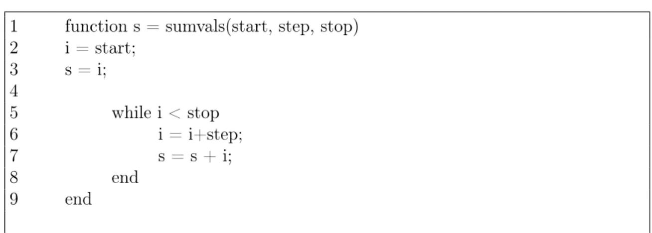
When removed, the identified aspects, as we see in Fig. 3.3, the LOC of ’sumvals’ function is 9, with this we calculate the Aspect Impact LOC, which is 9

12 = 0.75 • Aspectual Bloat [18] measure the aspects in terms of LOC bloat in the MATLAB

programs, and is calculated by the following formula:

LOC MATLAB − LOC without concerns LOC o f aspects

(46)

when the result is 1, means that the number of lines of aspect plus the the number of lines of the MATLAB program without aspects is the same that the number of lines of the MATLAB program with aspects.

When the the result is bigger then 1, means that the number resulting by the di ffer-ence of number of lines of MATLAB programs with and without aspects, is bigger than the number of lines of aspects, i.e., the same aspects appear more then once in the same program, like logging in Fig. 3.2.

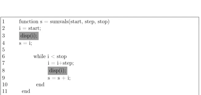
1 function s = sumvals(start, step, stop) 2 i = start; 3 disp(i); 4 s = i; 5 6 while i < stop 7 i = i+step; 8 disp(i); 9 s = s + i; 10 end 11 end

Figure 3.2: Sumvals function with logging

applying this metrics on the example of the Fig. 3.2, where we have the same disp com-mand twice in the ’sumvals’ program, we get the following result:

11 − 9 1 = 2

(47)

3.4. RESULTS OF METRICS FOR ASPECTS 33 1 function s = sumvals(start, step, stop)

2 i = start; 3 s = i; 4 5 while i < stop 6 i = i+step; 7 s = s + i; 8 end 9 end

Figure 3.3: ’Sumvals’ function without concerns

3.4 Results of Metrics for Aspects

The table 3.1 presents the results of aspect metrics applied to the same programs on the Chap. 2.

(48)

Function package Concern Impact Tangling Ration Concern Diffusion over LOC Aspectual Bloat

fdyn2.m Robotic 0.92 7.00% 1 1.5

ftrans.m Robotic 1 0.00% 0 N/A

gravload.m Robotic 0.71 28.86% 2 2.25

ishomg.m Robotic 1 0.00% 0 N/A

isvec.m Robotic 0.69 39.23% 4 2.25

itorque.m Robotic 1 0.00% 0 N/A

motomanhp.m Robotic 1 0.00% 0 N/A

roty.m Robotic 1 0.00% 0 N/A

standford.m Robotic 0.666 33.33% 2 1 startup.m Robotic 1 0.00% 0 N/A t2r.m Robotic 0.5 50.00% 4 2 tr2angvec.m Robotic 0.904 4.00% 2 3 tr2diff.m Robotic 0.666 22.22% 2 2.25 tr2jac.m Robotic 1 0.00% 0 N/A trplot.m Robotic 0.66 26.66% 4 1.67 uninorm.m IMPACTED 0.9577 2.00% 2 1.35

track_sites_error.m IMPACTED 1 0.00% 0 N/A load_map_files.m IMPACTED 0.678 7.00% 2 2.33

hybrid.m IMPACTED 1 0.00% 0 N/A

hist_rank.m IMPACTED 1 0.00% 0 N/A

historic_error.m IMPACTED 1 0.00% 0 N/A get_thresholds.m IMPACTED 0.888 16.00% 3 1 get_retargeting.m IMPACTED 0.5 50.00% 4 1 get_nominalSite.m IMPACTED 0.44 22.22% 2 1 fuzzy_trap.m f IMPACTED 0.89 10.52% 2 1 find_pixel_regions.m IMPACTED 0.933 13.33% 2 1 dist_d.m IMPACTED 1 0.00% 0 N/A

decision_values.m IMPACTED 1 0.00% 0 N/A comp_weights.m IMPACTED 0.86 13.33% 2 1

build_regions.m IMPACTED 0.666 7.41% 2 3.5

build_dmap.m IMPACTED 0.92 15.38% 2 1

Table 3.1: Aspect metrics results

Observing the table 3.1, we see that in only eighteen out of thirty one MATLAB pro-grams analyzed have aspects (concerns). Analyzing these eighteen propro-grams where aspects were found, we can see through the Tanging Ratio that the code of the programs, are sig-nificantly polluted.

Nevertheless, if we look to results of CDLOC, we can see that the numbers of transition points in these MATLAB programs are not to big, so is obvious that the identified concerns are very concentrated in the code. A good example is the t2r.m program that has an Tanging Ratioof 50%, and an CDLOC of 4.

(49)

3.5. ASPECTED ORIENTED PROGRAMMING AOP 35

3.5 Aspected Oriented Programming AOP

Having computed the programs in our repository that have aspects, we can now further analyze them. This analysis consists on verifying which version of the MATLAB program is better, in terms of quality, but to do this we first have transform these programs into AOP equivalents, since, there is no automatic tool to perform this "aspectualization" we have done it manually. Them we apply the metric suite referenced in Chap. 2 in the MATLAB programs (without concerns) and in the aspects.

Once we have the results of each one, we will analyze, for each metric, if the AO version of the program is better than the original.

Function package LOC #operators #operands Voc PL CPL Vol Dif Effort C.C fdyn2.m Robotic 4 2 8 10 15 26 49.82 1.37 68.51 0 gravload.m Robotic 4 1 6 7 16 15.50 44.91 1.16 52.40 0 isvec.m Robotic 2 1 2 3 3 2 4.75 0.5 2.37 2 standford.m Robotic 2 2 2 4 11 4 22 3.5 77 0 t2r.m Robotic 2 0 1 1 1 0 0 0 0 2 tr2angvec.m Robotic 2 0 5 5 7 0 16.25 0 0 1 tr2diff.m Robotic 2 4 7 11 30 27.65 103.78 6.85 711.65 1 trplot.m Robotic 3 1 2 3 4 2 6.33 0.5 3.16 1 uninorm.m IMPACTED 26 12 8 20 150 67.01 648.28 71.25 46190.60 0 load_map_files.m IMPACTED 3 1 5 6 7 11.60 18.09 0.5 9.04 1 get_thresholds.m IMPACTED 2 1 2 3 5 2 7.92 0.75 5.94 0 get_retargeting.m IMPACTED 2 1 2 3 4 2 6.33 0.75 4.75 0 get_nominalSite.m IMPACTED 3 1 2 3 4 2 6.33 0.75 4.75 0 fuzzy_trap.m IMPACTED 3 1 4 5 9 8 20.89 0.87 1 8.28 3 find_pixel_regions.m IMPACTED 2 1 1 2 2 0 2 0.5 1 0 comp_weights.m IMPACTED 2 1 1 2 2 0 2 0.5 1 0 build_regions.m IMPACTED 2 3 3 6 10 9.50 25.84 2.5 64.62 0 build_dmap.m IMPACTED 1 1 2 3 4 2 6.33 0.75 4.75 0

(50)

Function package LOC #operators #operands Voc PL CPL Vol Dif Effort C.C. fdyn2.m Robotic 7 4 14 18 54 61.30 225.17 5.42 1222.38 1 gravload.m Robotic 5 1 5 6 20 11.60 51.69 1.7 87.88 1 isvec.m Robotic 8 2 7 9 17 21.65 53.88 1.71 92.38 0 standford.m Robotic 5 3 5 8 134 251.88 809.81 3.93 2943.64 0 t2r.m Robotic 4 2 4 6 12 10 31.01 2 62.03 0 tr2angvec.m Robotic 36 8 20 28 221 110.43 1062.42 32.2 34210.09 1 tr2diff.m Robotic 4 5 9 14 54 40.13 205.59 11.11 2284.41 1 tr2jac.m Robotic 4 3 7 10 69 24.40 229.21 10.5 2406.73 0 trplot.m Robotic 10 3 8 11 23 28.75 79.56 3 238.70 2 uninorm.m IMPACTED 36 11 14 25 251 91.35 1165.60 58.92 68687.60 8 load_map_files.m IMPACTED 21 5 15 20 73 70.21 315.50 8.16 2576.58 0 get_thresholds.m IMPACTED 16 4 19 23 122 88.71 551.87 8.52 4705.45 0 get_retargeting.m IMPACTED 6 4 8 12 45 32 161.32 7 1250.25 0 get_nominalSite.m IMPACTED 6 4 5 9 21 19.60 66.56 5.2 346.15 0 fuzzy_trap.m IMPACTED 17 12 13 25 114 91.12 529.39 35.07 18569.70 0 find_pixel_regions.m IMPACTED 15 7 12 19 89 62.67 378.06 18.95 7167.49 1 comp_weights.m IMPACTED 13 4 9 13 43 36.52 159.11 6.44 1025.43 1 build_regions.m IMPACTED 20 8 19 27 82 104.71 389.90 10.73 4186.30 1 build_dmap.m IMPACTED 12 4 9 13 33 36.52 122.11 5.11 624.14 2

Table 3.3: Metrics results of programs without Concerns

Please note we are using real application/library where no logging was performed. As it is widely known, logging is "the" example of AOSD, and we are convinced that better results will be achieved in that context.

With the results presented in Tab. 3.2 and Tab. 3.3, we are now able to compare the original MATLAB programs with its AO version. To do that we will sum, for each metric, the results of the AO version, i.e., we sum the results obtained for MATLAB programs without concerns with the results obtained for the aspects, and once we have these values we will than compare them with the values of Tab. 2.1 and see which of them, original or AO version, has better quality. This analysis will allow us to verify when it is worth the use of AOP in MATLAB programs.

(51)

3.5. ASPECTED ORIENTED PROGRAMMING AOP 37

Function package LOC #operators #operands Voc PL CPL Vol Dif Effort C.C. fdyn2.m Robotic 11 4 16 20 69 87.30 274.99 6.79 1290.89 1 gravload.m Robotic 9 3 9 11 36 27.10 96.60 2.86 140.28 1 isvec.m Robotic 10 2 8 10 20 23.65 58.63 2.21 94.75 2 standford.m Robotic 6 3 5 8 145 255.88 831.81 7.43 3020.64 0 t2r.m Robotic 6 2 5 7 13 10 31.01 2 62.03 2 tr2angvec.m Robotic 38 8 20 28 228 110.43 1078.67 32.2 34210.09 2 tr2diff.m Robotic 6 6 9 15 84 67.78 309.37 17.96 2996.06 1 trplot.m Robotic 13 3 8 11 27 30.75 85.92 3 .5 241.86 1 uninorm.m IMPACTED 62 12 14 26 401 158.36 1813.88 130.17 114878.2 8 load_map_files.m IMPACTED 24 5 16 21 80 81.81 333.59 8.66 2585.62 1 get_thresholds.m IMPACTED 18 4 20 24 127 90.71 559.79 9.27 4711.62 0 get_retargeting.m IMPACTED 8 4 9 13 49 34 167.65 7.75 1255 0 get_nominalSite.m IMPACTED 9 4 6 10 25 21.60 72.89 5.95 350.9 0 fuzzy_trap.m IMPACTED 19 12 13 25 123 99.12 550.28 35.94 18577.98 3 find_pixel_regions.m IMPACTED 17 7 12 19 91 62.67 380.06 19 7168.49 1 comp_weights.m IMPACTED 15 4 9 13 45 36.52 161.11 6.94 1026.43 1 build_regions.m IMPACTED 22 9 19 28 92 114.21 415.4 13.23 4250.92 1 build_dmap.m IMPACTED 13 4 9 13 37 38.52 128.44 5.86 628.89 2

Table 3.4: Sum of the Tab. 3.2 and Tab. 3.3 (AO version)

3.5.1 Results represented in graphics

To compare the results of Tab 2.1 with the results of Tab. 3.3, we will consider each metric and present it in an bar chart. This kind of illustration allows to analyze the results for each metric an each program.

For each chart we will interpreting/analyze the behavior of the values in the both versions of programs, and try to get any conclusion of where the AOP for MATLAB is a better approach than the traditional approach for MATLAB programming, i.e, which of the two versions gives us more quality.

(52)

fd yn 2 gra vl oa d isve c st an df ord t2r tr2 an gve c tr2 di ff trp lo t un in orm lo ad _ma p_ fil e ge t_ th re sh ou ld s ge t_ re te rg et in g ge t_ no mi na lsi te fu zzy_ tra p fin d_ pi xe l_ re gi on co mp _w ei gh t bu ild _re gi on s bu ild _ma p 0 10 20 30 40 50 60 70 Original MatLab MatLab + Aspects

Figure 3.4: LOC values of the original MATLAB and the AO version

Fig. 3.4, present the chart of the comparison of the LOC values between the original MATLAB programs and the AO versions. Looking to the chart we see that in general way, the use of AOP in MATLAB is beneficial, once that in this case, the worst scenario is when the LOC value is the same as the original MATLAB . For all the other cases we observe an gain in the LOC value when we used this approach, translating this to numbers, ten of the eighteen programs analyzed showed improves for this metric when used the AO versions of the programs.

(53)

3.5. ASPECTED ORIENTED PROGRAMMING AOP 39 fd yn 2 gra vl oa d isve c st an df ord t2r tr2 an gve c tr2 di ff trp lo t un in orm lo ad _ma p_ fil e ge t_ th re sh ou ld s ge t_ re te rg et in g ge t_ no mi na lsi te fu zzy_ tra p fin d_ pi xe l_ re gi on co mp _w ei gh t bu ild _re gi on s bu ild _ma p 0 2 4 6 8 10 12 Original MatLab MatLab + Aspects

Figure 3.5: Number of operators of the original MATLAB and the AO version

As it is shown in Fig. 3.5, the chart of the #operators values shows that in average the use, in terms of #operators, of AO MATLAB version brings no advantage, once the val-ues in both version of the programs are the same in most cases. Only two of the eighteen programs presented, the t2r and tr2angvec programs, have some gain when use the AOP approach.

(54)

fd yn 2 gra vl oa d isve c st an df ord t2r tr2 an gve c tr2 di ff trp lo t un in orm lo ad _ma p_ fil e ge t_ th re sh ou ld s ge t_ re te rg et in g ge t_ no mi na lsi te fu zzy_ tra p fin d_ pi xe l_ re gi on co mp _w ei gh t bu ild _re gi on s bu ild _ma p 0 5 10 15 20 Original MatLab MatLab + Aspects

Figure 3.6: Number of operands of the original MATLAB and the AO version

Fig. 3.6 shows a total balance in the values of #operands in both versions in all pro-grams. In this case the AOP approach for MATLAB does not changes the quality, in terms of #operands values, of the originals MATLAB programs.

(55)

3.5. ASPECTED ORIENTED PROGRAMMING AOP 41 fd yn 2 gra vl oa d isve c st an df ord t2r tr2 an gve c tr2 di ff trp lo t un in orm lo ad _ma p_ fil e ge t_ th re sh ou ld s ge t_ re te rg et in g ge t_ no mi na lsi te fu zzy_ tra p fin d_ pi xe l_ re gi on co mp _w ei gh t bu ild _re gi on s bu ild _ma p 0 5 10 15 20 25 Original MatLab MatLab + Aspects

Figure 3.7: Vocabulary values of the original MATLAB and the AO version

The chart of Vocabulary, Fig. 3.7, shows that in average the quality of both versions of the programs is the same, in only three programs we can observe some improvement in the quality in the AO version of the MATLAB program.

The programs are: gravload, t2r, tr2angvec, and as we can see the improvement is not very high, only one unit in each program, but enough to enhance the quality.