EPGE Escola Brasileira de Economia e Finanças N◦ 819 ISSN 0104-8910
Progressive Consumption Taxes
Carlos E. da Costa, Marcelo R. Santos
Setembro de 2020
URL: http://bibliotecadigital.fgv.br/dspace/handle/10438/544p. - (Ensaios Econômicos; 819)
Inclui bibliografia.
Carlos E. da Costa FGV EPGE [email protected] Marcelo R. Santos INSPER [email protected] September 29, 2020 Abstract
In a static setting, whether consumption or labor income is progressively taxed is irrelevant for household choices and welfare. In a dynamic setting, however, these two forms of progressivity have markedly different implications for how earnings vary along the life-cycle: in a stylized life-cycle model, progressive income tax act reducing Frisch elasticities of labor supply whereas progressive consumption taxes act reducing the elasticity of intertemporal substitution. After showing that the latter leads to less inefficiencies in the stylized model than the former, we explore the consequences of replacing the current U.S. tax system by one in which labor income are linear and con-sumption taxes are progressive. We find welfare gains that exceed 10% in concon-sumption equivalent variation terms for all possible specifications in steady state comparisons. Welfare gains are attained in all our specifications with either very small increases in the capital stock or even large declines. Keywords: Progressive consumption taxes; warm-glow motives. J.E.L. codes: E6; H3; J2.
F
undamental tax reform is once again a hot topic in policy debate due to the perva-sive inefficiencies and distortions that have been accumulating in the U.S. tax system. Among the most frequent advanced ideas is the move to a system more centered on con-sumption taxes. While we could refer toKaldor(1956), as an early reference to the idea of moving to a system based on consumption taxes the appeal of such taxes dates as far back as Thomas Moore, which in his masterpiece, Leviathan, states, "It is fairer to tax people on what they extract from the economy, as roughly measured by their consumption, than to tax them on what they produce for the economy as roughly measured by their income."Despite these views, the idea of moving to a system mostly based on consumption taxes is usually held back by its alleged regressivity. The goal of this paper is to study the potential
da Costa gratefully acknowledges financial support from CNPq Proc. 301140/2017-0. Santos gratefully acknowledges financial support from CNPq Proc. 311437/2014-1. We thank Pedro Cavalcanti, Felipe Iachan, Cézar Santos and participants at the EPGE FGV Macro Group. All errors are our sole responsibility.
benefits from moving to a consumption based tax system that addresses its main shortcom-ing; we study a reform that replaces progressive income taxes by progressive consumption taxes.
In a static world, labor income and consumption taxes are equivalent. Simplicity, ad-ministrative ease, and many of the important issues related to real world tax systems dis-cussed bySlemrod and Gillitzer(2014), should ultimate determine which system is best. Although we acknowledge that these considerations may justify or undermine a reform, we shall not have much to add to the subject. Instead, we focus on the different implica-tions of these two types of progressivity in a dynamic setting. As we shall try to convey the potential benefits of progressive consumption taxes are so large as to justify a careful evaluation of its practical implementation.
BothKaldor(1956) andHall and Rabushka(2007) take income taxes to mean taxes on both labor and capital income, with a consequent focus on the reform’s impact on savings. We, instead, distinguish labor and capital income taxes and assume that progressivity only applies to the former in the benchmark. That is not to say that the consequences of our re-form are not important as we shall see. Another important aspect of our analysis is that we do not take into account the confiscatory aspect of a non-anticipated move to consumption taxes emphasized byCorreia(2010), for example; our analysis is centered in steady state comparisons.
So, what are the forces that we explore here? First, note that the novelty of our work is to introduce progressivity in consumption taxes. Again, in a static world, whether we intro-duce progressivity in income taxes – concave earnings retention function – or in consump-tion – concave mapping from expenditures to consumpconsump-tion – is immaterial. The effects highlighted in this paper only arise when the intertemporal nature of household choices are taken into account. If labor income taxes are progressive, more taxes are paid when earnings are higher, whereas, when it is consumption taxes which are progressive, more taxes are paid when consumption is higher. This has important allocative consequences.
Indeed, consider the progressive tax schedules studied byHeathcote et al.(2017b)– henceforth HSV schedules, 𝑇(𝑧) = 𝑧 − 𝜉𝑧1−𝜏, where 𝑧 is labor income. In a very styl-ized life-cycle model – Section1, we show that the main consequence of such taxes for household behavior is to reduce the Frisch elasticity of labor supply, making agents less responsive to the evolution of productivity that takes through one’s life. The allocation of time or effort across ages is therefore distorted. When this system is replaced with one in which progressivity is on consumption taxes efficient intertemporal allocation of effort is restored. The downside is that we increase the intertemporal elasticity of substitution, thus increasing the desire for consumption smoothing.
The main goal of this paper is to provide a quantitative assessment of such reform, under more realistic conditions. We calibrate an overlapping generations economy where agents live a meaningful life-cycle facing shocks to their labor market productivity while self in-suring through imperfect capital markets. While the progressivity of the current tax system provides insurance against earnings fluctuation, a progressive consumption schedule pro-vides insurance against consumption fluctuation.
We find very large welfare gains.1 Although large gains are due to the effects we have anticipated in our discussion, a very large impact of consumption tax progressivity on sav-ings cannot be a priori discounted. To understand the logic, it is important to mention that agents in our model save not only for smoothing purposes but also because they de-rive direct utility from wealth accumulation through a warm glow motive. Such feature is introduced to account for the empirical wealth distribution. Indeed, non-homethetic util-ity for wealth has been incorporated in many macroeconomic models to account for the convexity of savings with respect to permanent income, an empirical regularity recently competently explored byStraub(2019), and its consequence for wealth accumulation.2 As it turns, a progressive consumption tax leads the very rich to save even more. Because wealth is not ’eaten away’ by the rich, they sacrifice more consumption which is not only turned into more capital accumulation but also left for the poor, thus strengthening the dis-tributive (in terms of consumption Gini) impact of such reform. Yet, what we find in our baseline reform is that the capital stock increases by only 2.2% which can hardly explain the sizable gains we find.3
Still, since there is no consensus regarding the elasticity of bequest motives with respect to consumption taxes we run various robustness exercises.4 The exact value of welfare gains varies substantially across specifications but they remain very high in all exercises. In particular, when we assume that donors derive utility not by the bequest they leave but by the amount of consumptions that the donee can guarantee him or herself with the inherited bequest, welfare gains drop to 10.95% despite a 8.45% decline in the capital stock. All variations considered welfare gains vary – from a minimum gain of 8.62% to a
max-1
In our baseline example, the unconstrained optimum generates a welfare gain of 13.34%. To put in per-spective,Conesa et al.’s (2009) highly cited work finds a 1.33% gain.Kapička’s (2020) introduction of history dependence on income taxes attains a maximum gain of 2.98%. Conesa et al.(2020a), 5.47% with differenti-ated commodity taxes, andConesa et al.(2020a), 5.96% with differentiated taxes and a very generous Universal Basic Income.
2Straub(2019) shows how this convexity can partially account for the recent decline in real interest rates, the rising private wealth to GDP ratio and the fast increase in wealth inequality in the U.S.
3Again, it is useful to compare withConesa et al.(2020a) andConesa et al.(2020b) where large gains are also obtained. InConesa et al.(2020b), the 5.96 increase in welfare is mostly explained by a 29.8% capital stock increase. These large increases in capital stock lead welfare gains to be more than dissipated in the transition. 4Unfortunately, most of the literature has emphasized the bequest responses to estate taxes, and we know of no study that directly explores responses to consumption taxes. AsKopczuk(2013) emphasizes, modeling details matter, and absent more evidence one has to focus on results which are robust across specifications.
imum gain of 14.49%. The lowest value arises when we restrict policies to those that do not increase the share of revenues raised by consumption taxes. This is a strong arbitrary restriction on tax instruments which induces an 18% decline in capital stock, which sug-gest large ’extra’ welfare gains in a transition for the new steady state. If we allow the U.S. to become more like the rest of the OECD with regards to the relevance of consumption taxes, then steady state welfare gains return to two digits.
Following a brief literature review, in Section1we use a stylized model to provide the heuristics of our main results. Section2is where we write down and calibrate to the U.S. economy a model where agents live a meaningful life-cycle, are exposed to earnings risk, and face imperfect capital markets. In Section3we display our main results, which have their robustness assessed is Section4. Section5compares our findings with those ofConesa et al.(2020a,b) where progressivity is attained by differentiated taxation of commodities. Section6is of a very speculative nature. There we digress about the difficulties associated with the practical implementation of progressive consumption taxes. Finally, Section 7 concludes.
Brief Literature Review
This paper is about fundamental tax reform. FamouslyVickrey’s (1947) "Agenda for Pro-gressive Taxation" proposed replacing the yearly basis for income taxation by a tax system based on the notion of income averaging. More recently, the idea of transitioning to a consumption based tax system has found some support in a great deal due toHall and Rabushka’s (2007) flat tax andBradford’s (2005) X-tax proposals. We follow their lead in proposing a large overhaul in the U.S. tax system, but focus on the quantitative assessment of such reforms.
The focus on consumption taxes has its roots on actual proposals as the aforementioned flat tax and X-tax ideas. Of course, advocacy of consumption taxes dates back as far as Thomas Hobbes’, while its potential regressivity was already recognized by John Stewart Mill (cite).5We consider a model in which this regressivity is present. We allow agents to derive direct utility from accumulating wealth through a warm-glow bequest motive, first used byAndreoni(1989,1990). By introducing non-homotheticity in these preferences we make consumption concave in permanent income, as shown byStraub(2019), and approx-imate the distribution of wealth found in the data, e.g.,De Nardi(2004).
Non-homotheticity of warm-glow motives causes life-time-richer agents to consume a lower fraction of their life-time income than poorer agents, hence producing the type of regressivity that is referred to by the literature. What we do in this paper is to allow policy to impose progressivity directly on consumption taxes. This again has ancient roots. After
5 Mill
pointing our the potential regressivity of consumption taxes, John Stewart Mill suggested the exemption of necessities as a way of introducing progressivity in consumption taxes. The idea of consumption tax progressivity was not abandoned, and many proposals have been advanced in the more than 150 years that has elapsed since Mill’s work. In most cases, progressivity was attained in most proposals by a combination of income taxes (taxes on 𝑧𝑡+𝑟𝑡−1𝑎𝑡−1) with investment expenses (subsidies on 𝑎𝑡−𝑎𝑡−1). Our work is agnostic about
how progressivity is attained and we simply assume that it is equally feasible to introduce progressivity on income and on consumption taxes.
In a provocative post dating back a few years, John Cochrane proposes replacing the U.S. current income tax schedule by a progressive Value Added Tax. His main motivation is that by doing so many of the features that are added to the income tax system can be avoided and the tax code simplified. In his words, “An income tax made sense in 1914, when it was a small tax aimed only at high incomes, and when incomes were much easier to measure than consumption. But that is no longer the case.” He continues, " We have a sales tax reporting mechanism, so adding or substituting VAT tax reporting is not that hard.”6 Our work is silent about whether this view has merit. Indeed our approach does not capture the practical implementation issues that arise when one takes the tax system perspective, in the sense ofSlemrod and Gillitzer (2014), and motivate Cochrane’s post. For our purposes, any combination of taxes that lead to the budget constraints we evaluate here is equally valid.7
The main source of inefficiency that the schedules we study try to avoid are related to the allocation of effort across ages and states of nature. Along these lines, our work is rem-iniscent ofVickrey’s (1947) income averaging approach. In a very stylized model we show that his proposal dominates ours since ours trades-off intertemporal distortions in effort and in consumption, whereasVickrey’s proposal is based on the lifetime value of both con-sumption and income, thus avoiding all intertemporal distortions.Kapička(2020), which is a modern take on these types of fundamental tax reforms, shows that, when compared to a history dependent tax,Vickrey’s proposal remain optimal if productivity shocks are only transitory.
Since we add to bothVickrey’s andKapička’ life-cycle models a warm glow bequest motive progressive consumption taxes may have a very important role in incentivizing sav-ings when such a motive for wealth accumulation is present. We use different elasticities of bequests with respect to consumption taxes and consider many restrictions on the al-lowable schedules to assess the robustness of our findings. For all optimal schedules and
6https://johnhcochrane.blogspot.com/2017/04/a-progressive-vat.html. 7
Although the tax system which mimics consumption taxes by adding investment expenses to the income tax schedule is not a perfect substitute for the one analyzed here, one can think of adding features that make them so. E.g., by allowing income taxes to depend on investments and investment subsidies to depend on income.
all specification of preferences we find very large welfare gains.
The use of warm-glow preferences raises some important issues regarding the welfare criterion to be used — e.g., Diamond(2006);Kopczuk(2013). We take the conservative view of ignoring the flow utility generated by warm-glow.
By moving from income to consumption taxes a concern regarding policy evaluation is the role of wealth confiscation as emphasized byCorreia(2010). We avoid this issue by focusing on steady-state comparisons.
Closest to our work isConesa et al.(2020a,b). Progressivity in consumption taxes is attained in their model through the differentiated taxation of luxuries and necessities. The problem with such way of generating progressivity is that it is highly inefficient. Indeed, they consider preferences which are separable between consumption goods and leisure. A direct application ofCorlett and Hague’s (1953) classic result prescribe taxing more heavily the necessity. By subsidizing the good that should be taxed by purely efficiency reasons, one incurs in huge inefficiencies to attain redistribution. Again, our proposal avoids this drawback by directly imposing progressivity on all consumption.
Although we do not evaluate the transition to the new steady state, the welfare gains we find arise with either very little increase in the capital stock or even large declines. This suggests that the transition costs that undermine all reforms inConesa et al.(2020a) and Conesa et al.(2020b) should not occur here.
1
Heuristics
The purpose of this section is to clarify the conceptual difference between consumption tax progressivity and labor income tax progressivity. We organize our discussion around constant progressivity schedules – 𝑇(𝑧) = 𝑧 − 𝜉𝑧1−𝜚, where 𝑧 are earnings.8 Parameter 𝜚 controls progressivity and 𝜉 is used to adjust the level of taxes. We shall refer to these schedules as HSV schedules in reference toHeathcote et al.(2017b), who has advocated its use as a good approximation of the U.S. system.
Let ̂𝑐 denote the agent’s expenditure and 𝑐, his consumption. In a static world, we have 𝑐 = ̂𝑐 ≤ 𝜉𝑧1−𝜚. Such budget constraint is, of course, equivalent to 𝑐 ≤ 𝜉 ̂𝑐1−𝜚 = 𝑧, in which labor income is no longer taxed while consumption expenditures are now progressively taxed. Since the budget sets are identical, the two systems are equivalent.
In a multi-period model, however, we can write ∑
𝑡
̂𝑐𝑡− 𝑦𝑡 (1 + 𝑟)𝑡 ≤ 0,
8Musgrave(1959);Feldstein(1969) which represent early uses of this parametrization for income tax sched-ules, emphasize their constant progressivity.
where ̂𝑐𝑡denotes period 𝑡 expenditures and 𝑦𝑡, period 𝑡 disposable income.
Typically, it is income which is progressively taxed. In which case, ̂𝑐𝑡 = 𝑐𝑡 and 𝑦𝑡 =
𝜉𝑧1−𝜚𝑡 . Note that we could equivalently have allowed for linear consumption taxes, by mak-ing ̂𝑐𝑡= 𝑐𝑡(1 + 𝜏𝑐) and defining ̂𝜉 = 𝜉(1 + 𝜏𝑐). That is, whether the level parameter applies
to consumption or income is irrelevant for the agent’s program.9
But progressivity does matter. Indeed, consider the alternative tax system for which 𝑐𝑡 = 𝜉 ̂𝑐1−𝜚𝑡 and 𝑦𝑡 = 𝑧𝑡. Now, more taxes are paid in periods in which the agent’s con-sumption is higher, instead or periods in which earnings are higher. If we specialize our discussion to preferences of the form
𝑢(𝑐) = 𝑐
1−𝜎
1 − 𝜎 ℎ(𝑛) = 𝑛1+𝛾
1 + 𝛾,
then it is not hart to see that a progressive income tax schedule reduces the Frisch elasticity
of labor supply from 1∕𝛾 to (1 − 𝜚)∕(𝛾 + 𝜚), making labor supply more stable along the
life-cycle. As for progressive consumption taxes reduce the intertemporal elasticity of substitution from 1∕𝜎 to (𝜎(1 − 𝜚) + 1)∕(1 − 𝜚), while leaving the Frisch elasticity unaltered.
The allocative consequences of the two types of progressivity are different and we shall now offer a very stylized framework to compare the two. In our quantitative assessments the forces isolated in this section are shown to be very important in a more realistic setting – see Figure2.
We start by recalling that the dynamic problem has a static representation in which the agent derives utility from the present value of his or her consumption and, for each present value of income must endure some utility cost.
To simplify the notation, consider the no tax program under the assumption that 𝛽(1 + 𝑟) = 1, max 𝑇 ∑ 𝑡=1 𝛽𝑡−1[𝑢(𝑐 𝑡) − 𝑣(𝑛𝑡)] s.t. 𝑇 ∑ 𝑡=1 𝛽𝑡−1[𝑐 𝑡− 𝑛𝑡𝑤𝑡] ≤ 0.
It can equivalently be written as
𝑉(𝐶, 𝑍, 𝑊) = 𝐴−1max 𝐶≤𝑍 [ 𝐶1−𝜎 1 − 𝜎 − 𝐴 1 + 𝛾 ( 𝑍 𝑊) 1+𝛾 ] , for 𝐶 = 𝑇 ∑ 𝑡=1 𝛽𝑡𝑐𝑡, 𝑍 = 𝑇 ∑ 𝑡=1 𝛽𝑡𝑛𝑡𝑤𝑡, 𝑊 = ⎡ ⎢ ⎣ 𝑇 ∑ 𝑡=1 𝛽𝑡𝑤 1+𝛾 𝛾 𝑡 ⎤ ⎥ ⎦ 𝛾 1+𝛾 , 𝐴 = [1 − 𝛽 𝑇 1 − 𝛽 ] −𝜎 . 9
The constant 𝐴 accounts for the intertemporal aggregation: the ’technologies’ for i) converting, for a given life-cycle productivity profile, {𝑛𝑡}𝑡, a flow of effort costs (1+𝛾)
−1{𝑛1+𝛾 𝑡
}
into a present value of earnings, 𝑍, and; ii) converting a present value of earnings into a flow of consumption utilities, (1 − 𝜎)−1
{ 𝑐1−𝜎}
𝑡. This intertemporal aggregation in itself
may lead to more or less effort by this ’static’ representation of an agent making dynamic choices when compared to the same agent making true static choices, e.g., were he or she not able to access asset markets. When 𝑤𝑡is constant, if can be shown that whether more
or less effort is generated only depends on whether 𝜎 ⪋ 1. If 𝑢(𝑐) = ln 𝑐 intertemporal ag-gregation is irrelevant; the static representation of the dynamic problem leads to the same choices as the static problem. Note that there is nothing economically meaningful in this equivalence, it is just an adjustment which is necessary for a representation choice which is convenient for our discussion.
We can construct similar problems for the cases in which the budget constrains are
∑ 𝑡 𝛽𝑡[𝑐𝑡− 𝜉(𝑛𝑡𝑤𝑡)1−𝜚 ] ≤ 0, and ∑ 𝑡 𝛽𝑡[𝜉 1 𝜚−1𝑐 1 1−𝜚 𝑡 − 𝑛𝑡𝑤𝑡] ≤ 0, respectively.
A little algebra allows us to show that a progressive labor income tax is translated in the static model into a progressive static income tax 𝑇(𝑦) = 𝑦 − 𝜉𝑦1−𝜚 and a change in productivity. That is, under the progressive income the consumer solves
𝑉(𝐴, ̃𝑊) = 𝐴−1 max 𝐶≤𝜉𝑍1−𝜚[ 𝐶1−𝜎 1 − 𝜎 − 𝐴 1 + 𝛾( 𝑍 ̃ 𝑊) 1+𝛾 ] , for ̃ 𝑊 = {∑𝛽𝑡𝑤 (1+𝛾)(1−𝜚) 𝛾+𝜚 𝑡 } 𝛾+𝜚 (1−𝜚)(1+𝛾) .
When progressive consumption is used instead, the consumer program becomes
𝑉( ̃𝐴, 𝑊) = ̃𝐴−1 max 𝐶≤𝜉𝑍1−𝜚[ 𝐶1−𝜎 1 − 𝜎 − ̃ 𝐴 1 + 𝛾( 𝑍 𝑊) 1+𝛾 ] , for ̃ 𝐴 = [1 − 𝛽 𝑇 1 − 𝛽 ] 𝜎+𝜚(1−𝜎) 1−𝜚 .
Both could be compared toVickrey’s income averaging proposal, in which neither 𝐴 nor 𝑊 are affected by progressive taxation. Indeed, let us consider the income averaging
tax system that defines the intertemporal budget constraint ∑ 𝑡 𝛽𝑡𝑐 𝑡≤ ̂𝜉 [ ∑ 𝑡 𝛽𝑡(𝑛 𝑡𝑤𝑡)] 1−𝜚 , where ̂𝜉 = 𝜉 [
(1 − 𝛿𝑇)/(1 − 𝛿)], guarantees that all sequences of constant earnings and consumption that are feasible in one system are also in the other two.
It is then possible to prove the following proposition.
Proposition 1 If, for all𝑡, (1+𝑟𝑡) = 𝛽−1thenVickrey’s income averaging and the progressive consumption systems lead to the same allocations. Moreover, both are strictly better than the one implemented by the progressive income tax schedule if𝑤𝑡is not constant.
When (1 + 𝑟𝑡) ≠ 𝛽−1, thenVickrey’s system is strictly better than both. With 𝛽 < (1 +
𝑟)−1, agents choose an increasing consumption profile. Progressive consumption taxes act as an increasing consumption tax, which, as is well known is equivalent to capital taxation. This leads to an inefficient use of resources attained through labor. When 𝛽 > (1 + 𝑟)−1 then it acts as a capital subsidy, also leading to inefficiencies. If progressive income taxes are used instead, the intertemporal inefficiency in labor supply applies even when wages are constant.
2
Model
The discussion in Section 1is based on an overly simplistic description of the economy made to isolate the key forces we want to study. We have assumed perfect capital markets, ruled out any type of uncertainty, and ignored any bequest motive capable of reproducing the pattern of inheritances found in the data. All these aspects will play a role as we assess the benefits of such a reform under a more realistic setting.
2.1 Demography
Each period, 𝑗, a new generation is born. Uncertainty regarding the time of death for each person is captured by the fact that each individual faces a probability 𝜓𝑡+1of surviving to
the age 𝑡 + 1 conditional on being alive at age 𝑡. Hence, an individual born in period 𝑗 is alive in period 𝑗 + 𝑡 with probability∏𝑡𝑘=1𝜓𝑘. We also assume that there is 𝑇 > 0 such
that 𝜓𝑇+1= 0.
We assume independence of individual death shocks and appeal to the law of large numbers to map the survival probability into the time invariant age profile of the popula-tion denoted {𝜇𝑡}
𝑇
years old in the population is found using the following law of motion 𝜇𝑡= 𝜓𝑡 1 + 𝑔𝑛𝜇𝑡−1 with 𝜇𝑡 ≥ 0, ∑𝑇 𝑡=1𝜇𝑡 = 1.
Our focus is on working lives, hence an agents life starts at the age 𝑡 = 20. We also consider 𝑇 = 90. For most of our analysis we will focus on the steady-state allocations. Since it greatly simplifies the notation we drop all time indices, 𝑗, from aggregate variables and use 𝑡 to represent age.
2.2 Technology
Technology is standard. The production side of the economy aggregates and the technol-ogy for producing the consumption good is summarized by a Cobb-Douglass production function with constant returns to scale. That is,
𝑌 = 𝐵𝐾𝛼𝑁1−𝛼
where 𝐾 is aggregate capital, 𝑁 is aggregate efficient units of labor, and 𝐵 is a scale param-eter. Every period, the standing representative firm solves the static optimization problem
max
𝐾,𝑁
{
𝐵𝐾𝛼𝑁1−𝛼− 𝛿𝐾 − 𝑤𝑁 − 𝑟𝐾}
where 𝑟 is the rental rate of physical capital and 𝑤 is the rental rate of efficiency units of labor, i.e. the wage rate. Note that we assume that the rental rate of capital is net of depreciation costs which are born directly by the firm.
The first order conditions for the firm’s profit maximization problem are,
(1 − 𝛼)𝐵𝐾𝛼𝑁−𝛼 = 𝑤, (1)
and
𝛼𝐵𝐾𝛼−1𝑁−𝛼− 𝛿 = 𝑟. (2)
2.3 Households
Preferences Individuals derive utility from consumption, 𝑐, and leisure, 𝑙. Preferences
Morgenstern utility function, 𝔼⎡⎢ ⎣ 𝑇 ∑ 𝑡=1 𝛽𝑡−1( 𝑡 ∏ 𝑘=1 𝜓𝑘) 𝑈𝑡(𝑐𝑡, 𝑙𝑡) ⎤ ⎥ ⎦ , (3)
where 𝛽 is the subjective discount factor, and 𝔼 is the expectation operator conditional on information at birth.
We allow preferences over consumption-leisure bundles to vary with age by indexing the flow utility by 𝑡. Specifically, flow utility is of the form
𝑈𝑡(𝑐𝑡, 𝑙𝑡) = (𝑐𝑡
1−𝜌𝑡𝑙𝜌𝑡
𝑡 )1−𝛾− 1
1 − 𝛾 , (4)
for 𝜌𝑡∈ (0, 1) ∀𝑡, 𝛾 > 0, 𝛾 ≠ 1.
The fact that we allow the marginal rate of substitution between leisure and consump-tion to vary with age gives us more degrees of freedom to try to match the behavior of hours along the life-cycle. As 𝜌 decreases, agents become more willing to forego leisure to ob-tain more consumption. Since lower 𝜌 implies higher (in absolute terms) Frisch elasticity of leisure, the two effects compound to generate more variation in the Frisch elasticity of labor supply.
Another issue raised by our choice of time-varying preferences is that for a given 𝑛, the marginal utility of consumption varies with age. A perfectly smooth profile would no longer be optimal even if hours were constant. This choice of preferences some care in measuring and reporting welfare gains.
Note also that this specification for preferences implies a Frisch elasticity of labor sup-ply which decreases with hours worked. Indeed, let 𝜖𝑓denote the Frisch elasticity of labor supply. Then,
𝜖𝑓𝑡 = (1 − 𝛾)(1 − 𝜌𝑡) − 1 𝛾
1 − 𝑛𝑡
𝑛𝑡
Elasticities are, of course, crucial in the determination of optimal taxes. So, under-standing how hours vary along the life-cycle will be important for welfare assessment.
Wealth in the Utility Function In order for the model to be able to reproduce the
observed wealth distribution observed, we assume that individuals derive utility from leav-ing a bequest, 𝑎, to their children
𝜈(𝑎) = 𝜂1(1 + 𝑎 𝜂2)
(1−𝛾𝑐)
. (5)
has been regaining traction in recent times. We motivate it through a utility from bequeath-ing which, first introduced byAndreoni(1989), has been called a ’warm glow’ or ’joy-of-giving’ motive. From the perspective of our work two things are of essence. First, it creates non-homotheticities that have been proven essential to generate a wealth distribution that is closer to what one observed in the data thanks to its functional form, described in (5), first proposed byDe Nardi(2004). Second, a typical warm glow motivation implies that it is the amount received by the donee that matters for the donor not the amount that is donated. An alternative view, sometimes referred to as ’capitalistic spirit’ in reference to Weber’s
’The protestant ethic and the spirit of capitalism’ implies the opposite. One may think that
the distinction is immaterial for our analysis since we do not consider estate taxation. Yet, when we move to a consumption based taxation the same amount of wealth bequeathed entails less consumption than in a world in which it is labor income that is taxed. Because neither of these reduced forms of capturing an independent desire for accumulation have a clear micro-founded basis, we do not have a clear guide for defining how bequests react to consumption taxes. So, while in our baseline case we assume preferences of the form (5) we also explore the alternative specification (15) in Section4.
Labor Supply and Retirement Every period, individuals choose labor supply,
consump-tion, and asset accumulation to maximize their objective, (3), subject to a budget constraint which we shall explain momentarily.
Each person has a unit time endowment which can be directly consumed in the form of leisure, 𝑙, or used in market related activities. An agent’s period-by-period time constraint is 𝑙𝑡+ 𝑛𝑡 = 1. An individual of age 𝑡 who works for 𝑛 hours supplies to the market a total
of 𝑛𝑡𝑠𝑡𝑒(𝑢+𝑧𝑡)efficiency units which are paid at a rental rate 𝑤. The variable 𝑢 ∼ 𝒩(0, 𝜎𝑢2)
is a permanent component of an individual’s skills. It is realized at birth and retained throughout one’s life. On the other hand, 𝑧 follows an AR(1) process, 𝑧𝑡 = 𝜑𝑧𝑧𝑡−1 + 𝜀𝑡,
with innovations 𝜀𝑡 ∼ 𝑁(0, 𝜎𝜀2).
Whereas 𝑢 aims at capturing the heterogeneity at birth, the most relevant source of welfare variation, 𝑧 is the main source of uncertainty affecting long term choices. The parameter 𝜑𝑧accommodates the empirically observed persistence of productivity shocks.
Finally, 𝑠𝑡is what we call the age-efficiency profile.
Labor productivity shocks are independent across agents. As a consequence, there is no uncertainty regarding the aggregate labor endowment even though there is uncertainty at the individual level. Retirement is mandatory at the age of 65, or 𝑡 = 46.
Asset Accumulation Besides choosing how much leisure to consume, individuals trade
a risk free asset which holdings we denoted by 𝑎𝑡. Asset holdings are subject to an
in assuming that agents are not allowed to contract debt at any age, so that the amount of assets carried over from age 𝑡 to 𝑡 + 1 is such that 𝑎𝑡+1 ≥ 0. Because no agent can hold a
negative position in assets at any time, we assume without loss that asset takes the form of capital, 𝑎𝑡 = 𝑘𝑡, as inAiyagari(1994).
As we shall make clear, there is exogenous (as well as endogenous) variation in produc-tivity along the life-cycle. Consumption smoothing thus provides a reason for one to ac-cumulate assets. Another aspect of choices is that individuals may resort to self-insurance to protect themselves against the uncertainty on labor income. Savings will be, to some extent, motivated by precautionary reasons. By precluding borrowing we potentially affect the valuation of future social security benefits as compared to what we would observe in a world with perfect capital markets.
In addition, households are born with initial wealth endowment 𝑎1drawn from an
en-dogenous distribution that integrates up to the overall amount of wealth bequeathed in the economy by the deceased households. In order to account for the intergenerational persistence in wealth inequality, we assume that the draw is correlated with the perma-nent compoperma-nent of the elderly’s skills. In particular, let ̂𝑎𝑢and 𝜎2𝑎̂
𝑢 denote the mean and
the variance of wealth bequeathed by the deceased households with permanent skill 𝑢, re-spectively. Thus, an agent at the first age with permanent skill 𝑢 draws her initial wealth from a log-normal distribution with mean ̂𝑎𝑢and variance 𝜎𝑎2̂
𝑢.
10
Budget Constraints To write each agent’s flow budget constraint we need to specify the
fiscal policy that is being used by the Government. In our case, it is important to distinguish between the current fiscal policy, needed to calibrate the model, and the ones we evaluate. The current tax system will be the benchmark for our studies.
2.4 The Government
Tax revenues are raised to finance an exogenous flow of expenditures, 𝐺, and possibly to cover the social security deficit. The government levies taxes on capital income, consump-tion, and labor income. We assume that capital income is taxed at a flat rate 𝜏𝑘. Labor
income taxes are given by 𝑇(𝑦) = max{𝑦 − 𝜉𝑦1−𝜚, 0}. This specification was first proposed byMusgrave(1959) and since adopted byFeldstein(1969);Bénabou(2000,2002);
Heath-10The reason why we model the intergenerational links in the form of both accidental and voluntary be-quests this way is to avoid the inclusion of an additional state variable regards to the parents ability as is done inDe Nardi(2004). We assess the importance of bequest for our results in section4.3.
cote et al.(2017a), to name a few. Similarly, consumption taxes are specified as 𝑇( ̂𝑐) = max ⎧ ⎨ ⎩ ̂𝑐 − ( ̂𝑐 1 + 𝜏𝑐 ) 1 1+𝜚𝑐 , 0 ⎫ ⎬ ⎭ , (6)
The government also runs a social security system with contributions and benefits that are equal in equilibrium. Retirement benefits are given by
𝑏(𝑥) = ⎧ ⎪ ⎪ ⎨ ⎪ ⎪ ⎩ 𝜃1𝑥, if 𝑥 ≤ 𝑦1 𝜃1𝑦1+ 𝜃2(𝑥 − 𝑦1), if 𝑦1≤ 𝑥 ≤ 𝑦2 𝜃1𝑦1+ 𝜃2(𝑦2− 𝑦1) + 𝜃3(𝑥 − 𝑦2), if 𝑦2≤ 𝑥 ≤ 𝑦𝑚𝑎𝑥 𝜃1𝑦1+ 𝜃2(𝑦2− 𝑦1) + 𝜃3(𝑦𝑚𝑎𝑥− 𝑦2), if 𝑥 ≥ 𝑦𝑚𝑎𝑥 (7)
where 𝑥 is the individual’s average life-cycle earnings and 𝜃1> 𝜃2 > 𝜃3.
The law of motion for 𝑥 is given by
𝑥𝑡+1=
[𝑡 − 1] 𝑥𝑡+ 𝜏𝑠𝑠min {𝑦𝑡; 𝑦max}
𝑡 , (8)
and 𝑥𝑇 = 𝑥.
In addition, government provides individuals a minimum consumption, 𝑐. We assume that transfers, 𝑡𝑟𝑎, are conditional on individuals available resources. In particular, follow-ing Hubbard et al. (1995), we specify:
𝑡𝑟𝑎 = max{𝑐 − [1 + (1 − 𝜏𝑘)𝑟] 𝑎 − ̃𝑦 + 𝑇( ̃𝑦), 0} (9)
This equation implies that government transfers fill the gap between illiquid resources – which may include not only wealth and labor income, but also other government trans-fers such as social security benefits - and the consumption floor. Thus, individuals can always consume at least 𝑐. Equation (9) is intended to be a model counterpart for means-tested programs such as Food Stamp, AFDC, Section 8 housing assistance, Medicaid and SSI.
Recursive Formulation of Households’ Problem
A crucial definition in all that follows is that of consumption expenditure, ̂𝑐, which is re-lated to consumption through 𝑐 = ̂𝑐 − 𝑇𝑐( ̂𝑐). Using the definition of ̂𝑐 above, we define the
agents’ budget constraint at individual state 𝜔𝑡∶= (𝑎𝑡, 𝑢, 𝑧𝑡, 𝑥𝑡) ∈ Ω as ℬ(𝜔) ∶= { ( ̂𝑐, 𝑎′, 𝑙) ∈ 𝑅2 +× [0, 1]|||| ̂𝑐 + 𝑎′≤ [1 + (1 − 𝜏𝑘)𝑟] 𝑎 + ̃𝑦 − 𝑇( ̃𝑦), ̃ 𝑦 = 𝑦 − 𝜏𝑠𝑠min {𝑦, 𝑦max} , 𝑦 = [1 − 𝑙]𝑠𝑒(𝑢+𝑧) } .
Let 𝑉𝑡(𝜔𝑡) denote the value function of an individual aged 𝑡 < 𝑇 + 1, where 𝜔𝑡 =
(𝑎𝑡, 𝑢, 𝑧𝑡, 𝑥𝑡) ∈ Ω is the individual state. If the agent has not yet attained the retirement age, his or her optimization problem at age 𝑡 can be recursively represented as follows. Let 𝜔′ = (𝑎′, 𝑢, 𝑧′, 𝑥′), then, 𝑉𝑡(𝜔) = max ( ̂𝑐,𝑎′,𝑙)∈ℬ(𝜔)𝑈𝑡(𝑐, 𝑙) + 𝛽𝔼𝑧′ [ 𝑉𝑡+1(𝜔′) ] , . (10)
Although we have only used individual state variables in 𝜔, prices are, of course, also relevant state variables. To solve the model we will need to find the equilibrium prices by explicitly taking into account how they enter the policy functions associated with (10). Still for economy in notation we drop them from 𝜔.
For retired agents, no labor supply decision is made. Moreover, we assume that, af-ter retirement agents start deriving utility from bequests as well. A retired agents’ value function is, therefore,
𝑉𝑡(𝜔) = max ( ̂𝑐,𝑎′,1)∈ℬ(𝜔)𝑈𝑡(𝑐, 1) + 𝛽 [ 𝜓𝑡+1𝔼𝑧′𝑉𝑡+1(𝜔′) + (1 − 𝜓𝑡+1)𝜈(𝑎′) ] . (11)
Finally, considering that agents die for sure at age 𝑇, we have 𝑉𝑇+1(𝜔𝑇+1) = 𝜈(𝑎). 2.5 Recursive competitive equilibrium
Recall that we are describing our economy in the steady state. This has allowed us to drop time subscripts and use 𝑡 to denote age, instead.
At each point in time, agents differ from one another with respect to age their age, 𝑡, and their individual state, 𝜔 = (𝑎, 𝑢, 𝑧, 𝑥). Agents of age 𝑡 identified by 𝜔, are distributed according to a probability measure 𝜆𝑡defined on Ω, as follows. Let (Ω, ϝ(Ω), 𝜆𝑡) be a
prob-ability space, where ϝ(Ω) is the Borel 𝜎-algebra on Ω: for each 𝜂 ⊂ ϝ(Ω), 𝜆𝑡(𝜂) denotes the
fraction of agents aged 𝑡 that are in 𝜂.
Given the age distribution, 𝜆𝑡, 𝑄𝑡(𝜔, 𝜂) induces the age 𝑡+1 distribution 𝜆𝑡+1as follows.
𝑄𝑡(𝜔, 𝜂) determines the probability of an agent at age 𝑡 and state 𝜔 to transit to the set 𝜂 at age 𝑡 + 1. 𝑄𝑡(𝜔, 𝜂), in turn, depends on the policy functions in (10), and on the exogenous
stochastic process for 𝑧.
apply to the economy under the policy experiments we run.
Definition Given the policy parameters, a recursive competitive equilibrium is a
col-lection of value functions {𝑉𝑡(𝜔)} , policy functions for individual asset holdings 𝑑𝑎,𝑡(𝜔),
for consumption 𝑑𝑐,𝑡(𝜔), for labor supply 𝑑𝑛𝑤,𝑡(𝜔), prices {𝑤, 𝑟}, age dependent but
time-invariant measures of agents 𝜆𝑡(𝜔), transfers 𝜖 such that:
i) {𝑑𝑎,𝑡(𝜔), 𝑑𝑛𝑤,𝑡(𝜔), 𝑑𝑐,𝑡(𝜔)} solve the dynamic problems in (10);
ii) individual and aggregate behaviors are consistent, that is:
𝐾 = 𝑇 ∑ 𝑡=1 𝜇𝑡 ˆ Ω 𝑑𝑎,𝑡(𝜔)𝑑𝜆𝑡 𝑁 = 𝑇 ∑ 𝑡=1 𝜇𝑡 ˆ Ω 𝑑𝑛𝑤,𝑡(𝜔)𝑠𝑡(𝜔) exp(𝑢 + 𝑧𝑡)𝑑𝜆𝑡 𝐶 = 𝑇 ∑ 𝑡=1 𝜇𝑡 ˆ Ω {𝑑𝑐,𝑡(𝜔)}𝑑𝜆𝑡;
iii) {𝑤, 𝑟} are such that they satisfy the optimum conditions (2) and (1); iv) The final good market clears:
𝐶 + 𝐺 + 𝛿𝐾 = 𝐾𝛼𝑁1−𝛼;
v) the probability measure 𝜆𝑡(𝜔) follows the law of motion:
𝜆𝑡+1(𝜂) = ˆ
Ω
𝑄𝑡(𝜔, 𝜂)𝑑𝜆𝑡 ∀𝜂 ⊂ ϝ(Ω);
vi) the overall amount of wealth bequeathed by the deceased households correspond to the aggregate initial wealth endowment:
𝜇1 ˆ Ω 𝑎1(𝜔)𝑑𝜆1= 𝑇 ∑ 𝑡=𝑇𝑟 𝜇𝑡 ˆ Ω (1 − 𝜓𝑡+1)𝑑𝑎,𝑡(𝜔)𝑑𝜆𝑡
vii) taxes are such that the government’s budget constraint, 𝑇 ∑ 𝑡=1 𝜇𝑡 ˆ Ω 𝑇 ( 𝑑𝑛𝑤,𝑡(𝜔)𝑠𝑡(𝜔) exp(𝑢 + 𝑧𝑡)− 𝑇𝑠𝑠(𝑑𝑛𝑤,𝑡(𝜔)𝑠𝑡(𝜔) exp(𝑢 + 𝑧𝑡)) )𝑑𝜆𝑡+ 𝜏𝑐𝐶 + 𝜏𝑘𝑟𝐾+ 𝑇 ∑ 𝑡=1 𝜇𝑡 ˆ Ω 𝑇𝑠𝑠 ( 𝑑𝑛𝑤,𝑡(𝜔)𝑠𝑡(𝜔) exp(𝑢 + 𝑧𝑡) ) 𝑑𝜆𝑡 = 𝐺 + 𝐵 (12)
are satisfied every period, where 𝐵 are the total benefits that are due, given the social security system that we consider.
Item (vii) is redundant if conditions (i)–(vi) hold.
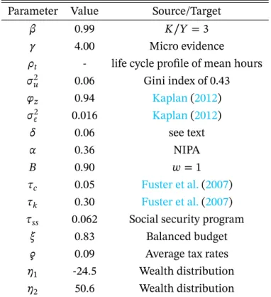
2.6 Calibration
To carry out our quantitative analysis, we need first to find values for all the parameters of the model. We accomplish this by calibrating the model to the U.S. economy.
The population age profile {𝜇𝑡} 𝑇
𝑡=1depends on the population growth rate, 𝑔𝑛, the
sur-vival probabilities, 𝜓𝑡, and the maximum age, 𝑇, that an agent can live. Agents enter the
economy at age 20 and live for 71 years, 𝑇 = 71, so that the real maximum age is 90 years. Data on survival probability by age were extracted fromBell and Miller(2005). Given the survival probabilities, the population growth rate is chosen so that the age distribution in the model replicates the dependency ratio observed in the data. By setting 𝑔𝑛 = 0.009,
the model generates a dependency ratio of 23.27%, which is close to the dependency ratio observed in the data for the year 2017.
To calibrate the preference parameters we proceed as follows. First, we choose the discount factor 𝛽 in such a way that the equilibrium of our benchmark economy implies a capital-output ratio around of 3.0, which is the value observed in the data. Then we fix the parameter 𝛾 to 4.0, from micro evidence, and choose the share of leisure in the utility function, 𝜌𝑡, to match average hours for different age groups. In particular, we assume that
𝜌𝑡 = 𝜌0+ 𝜌1𝑡. To calibrate 𝜌0, we use the average working hours for ages 19 − 40 and for
𝜌1the average between 41 − 60. The first group works on average 37.86 while the second 40.37 of their time endowment. For the last 5 years we specify a new profile 𝜌𝑡 = 𝜌60+ 𝜌2𝑡.
We calibrate 𝜌2to match the average hours during those last five years equal to 35.16.11
The parameter 𝜙1represents the weight on the utility from bequeathing. Since it
mea-sures the strength of bequest motives, we calibrate 𝜙1so that the ratio of the median wealth
held by the individuals aged 75 and above to that of all individuals is 1.8, as reported in the
11
Statistical Abstract of the United States (US Census Bureau 2009). The term 𝜙2is the shifter
of bequests in utility function. It reflects the extent to which bequests are luxury goods, af-fecting the bequest distribution, especially the high end of it. Thus, we followDe Nardi and Yang(2014) and set 𝜙2to match the 90th percentile of bequest distribution normalized by
income as reported by ?.
The parameters that characterized the stochastic component of individuals produc-tivity are (𝜎2𝑢, 𝜑𝑧, 𝜎𝜖2). Several authors have estimated similar stochastic process for labor
productivity. Controlling for the presence of measurement errors and/or effects of some observable characteristics such as education and age, the literature provides a range of [0.88, 0.96] for 𝜑𝑧and of [0.10, 0.25] for 𝜎2𝜖. In this article, we rely on the estimates of
Ka-plan(2012), setting 𝜑𝑧 = 0.94 and 𝜎𝜖2 = 0.016. Then, 𝜎2𝑢 was chosen for the Gini index
for labor income in the model to match its counterpart in the data, which is nearly 0.43. The value obtained for 𝜎2𝑢is in line with the estimates inKaplan (2012) who provides a
point estimate of 0.056 for this parameter. We discretize the two shocks in order to solve the model, using seven states to represent the permanent shock and eleven states for the persistent shock. For expositional convenience, we refer to the two extremes of the grid for the permanent shock as low and high ability type. We assume that individuals start the lifecycle with the mean level of the idiosyncratic shock 𝑧.
The values of the technological parameters (𝛼, 𝛿) are also in Table1. We chose a value for 𝛼 based on the U.S. time series data from the National Income and Product Accounts (NIPA). The depreciation rate, in turn, is obtained by 𝛿 = 𝐾∕𝑌𝐼∕𝑌 − 𝑔. We set the investment-product ratio 𝐼∕𝑌 equal to 0.25 and the capital-investment-product ratio 𝐾∕𝑌 equal to 3.0. The eco-nomic growth rate, 𝑔, is constant and consistent with the average growth rate of GDP over the second half of the last century. Based on data from Penn-World Table, we set 𝑔 equal to 2.3%, which yields a depreciation rate of 6.0%.
The age-efficiency profile for the exogenous model is set to be consistent with the values estimated inKaplan(2012), which are based on the average hourly earnings by age in the PSID. We use a second order polynomial to smooth this profile and extend it to cover ages from 16 to 65.
Finally, we specify the others parameters related to government activity. First, we set government consumption, 𝐺, to 18% of the output of the economy under the baseline cali-bration. Following the literature, we assume a consumption tax of 6% and a capital income tax rate of 30%.12 The parameter 𝜚, which governs the progressivity of the labor income taxes, is calibrated to match the actual average tax rates. Marginal tax rates are chosen to raise enough revenue to finance government consumption. The value we find for 𝜁 is 0.83.13
12See, for example,Fuster et al.(2007) 13Recall that 𝜁(1 − 𝜚)𝑦−𝜚
As for Social Security, we set the normal retirement age to 𝑇𝑟 = 46, which corresponds
to the real age of 65. Contributions are of the form 𝑇𝑠𝑠(𝑦) = 𝜏𝑠𝑠min {𝑦, 𝑦max}, where 𝑦maxis
the contribution ceiling. We set the payroll tax rate, 𝜏𝑠𝑠, to 6.2%. The marginal replacement
rates in the progressive Social Security payment schedule (𝜃1, 𝜃2, 𝜃3) are set at their actual
respective values of 0.9, 0.32 and 0.15. The bend points where the marginal replacement rates change (𝑦1, 𝑦2) and the maximum earnings 𝑦𝑚𝑎𝑥are set equal to the actual multiples
of mean earnings used in the U.S. Social Security system so that 𝑦1, 𝑦2and 𝑦𝑚𝑎𝑥occur at
0.21, 1.29 and 2.42 times average earnings in the economy.
3
Main Findings
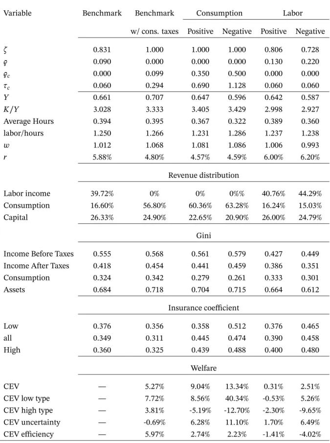
Our main findings are displayed in Table2. Before we discuss them it is necessary to define some key statistics.
Welfare The welfare variation (CEV) is calculated as follows: Let 𝑉1(𝜔) denote the
ex-pected utility of an agent who starts life at state 𝜔 under the policy we aim at evaluating. Then, define 𝑉10(𝜔) = 𝔼⎡⎢ ⎣ 𝑇 ∑ 𝑡=1 𝑡 ∏ 𝑠=1 𝜓𝑠(1 + ∆)(1−𝜌𝑡)(1−𝛾)𝑈 𝑡,0(𝑐𝑡, 1 − 𝑛𝑡) ⎤ ⎥ ⎦
where 𝑈1,0(𝑐𝑡, 1 − 𝑛𝑡) is the flow utility attained by the agent under the benchmark at age
t. Our relevant measure of welfare variation is
𝐶𝐸𝑉 = min
∆
[
𝔼𝜔𝑉10(𝜔) − 𝔼𝜔𝑉11(𝜔)]. (13)
Note how we take full advantage of our iso-elastic specification for preferences.
CEV Decomposition Aiming at understanding the source of welfare gains we
de-compose the CEV in variations that are due to improved insurance and those that are due to a more efficient use of aggregate resources. Let 𝐶0,𝑡and 𝐿0,𝑡denote average consumption
and average hours worked by 𝑡 years old agents at the benchmark, respectively. Let also 𝐶1,𝑡and 𝐿1,𝑡 denote the same statistics at the alternative tax system. We may, in this case,
implicitly define ∆𝑙𝑒𝑣through
∑ 𝑡 𝛽𝑡−1 𝑡 ∏ 𝑗=1 𝜓𝑡(((1 + ∆𝑙𝑒𝑣) 𝐶0,𝑡 )1−𝜌𝑡( 1 − 𝐿0,𝑡)𝜌𝑡) 1−𝛾 = ∑ 𝑡 𝛽𝑡−1 𝑡 ∏ 𝑗=1 𝜓𝑡 ( 𝐶1−𝜌𝑡 1,𝑡 ( 1 − 𝐿1,𝑡)𝜌𝑡 )1−𝛾 .
For (𝑐𝑡,0, 𝑙𝑡,0)𝑡, the benchmark equilibrium allocations, and (𝑐𝑡,1, 𝑙𝑡,1)𝑡, the equilibrium
allocations under the alternative policy, implicitly define 𝑝0and 𝑝1, through
∑ 𝑡 𝛽𝑡−1 𝑡 ∏ 𝑗=1 𝜓𝑡(((1 − 𝑝0) 𝐶0,𝑡 )1−𝜌𝑡( 1 − 𝐿0,𝑡)𝜌𝑡) 1−𝛾 = 𝔼⎡⎢ ⎣ ∑ 𝑡 𝛽𝑡−1 𝑡 ∏ 𝑗=1 𝜓𝑡 ( 𝑐1−𝜌𝑡 𝑡,0 ( 1 − 𝑙𝑡,0)𝜌𝑡 )1−𝛾⎤ ⎥ ⎦ , and ∑ 𝑡 𝛽𝑡−1 𝑡 ∏ 𝑗=1 𝜓𝑡( ( (1 − 𝑝1) 𝐶1,𝑡 )1−𝜌𝑡( 1 − 𝐿1,𝑡 )𝜌𝑡 ) 1−𝛾 = 𝔼⎡⎢ ⎣ ∑ 𝑡 𝛽𝑡−1 𝑡 ∏ 𝑗=1 𝜓𝑡 ( 𝑐1−𝜌𝑡 𝑡,1 ( 1 − 𝑙𝑡,1 )𝜌𝑡)1−𝛾⎤ ⎥ ⎦ , .
In both expressions 𝔼 denotes the unconditional expectation operator.14 Then,
∆𝑢𝑛𝑐 ≡ 1 − 𝑝1 1 − 𝑝0
− 1.
It is important to note that ∆𝑢𝑛𝑐only takes into account smoothing across agents of the
same age. The fact that preferences are age-dependent implies that complete smoothing across ages is not optimal.
Warm Glow and Welfare The use of a warm glow bequest motive some subtle
is-sues for normative analysis. In particular, should the utility gain from bequeathing be included in welfare evaluation?
In contrast with other form of externalities, if it is the act of bequeathing that is valued by agents, then the final allocation of resources need no longer suffice to define welfare. AsDiamond(2006) explains. "The mathematical formulation of warm glow preferences would also apply to a particular structure of ordinary externalities. In that case, we would count the utility of own consumption, w. What distinguishes a warm glow, and so the question of design of the social welfare function, is the distinction that actual resource use is the same with public and private public good supply, but individual experience is different in these two cases."
At the end of the day, the normative criterion choice matters for welfare evaluation. As is apparent from (13) the welfare assessment we use ignores the intrinsic (warm glow)
14
utility derived from the act of bequeathing. If we consider aggregate welfare gains, our measure is probably on the conservative side for the type of reform we study. It may, how-ever, bias how we measure the distribution of gains against the richest agents.
Insurance To assess the amount of consumption insurance for each possible policy we
define
𝜙 = 1 − Cov(𝑑 ̃𝑐𝑖,𝑡, 𝑑𝑧𝑖,𝑡)
Var(𝑑𝑧𝑖,𝑡) (14)
where ̃𝑐 = log(𝑐). The statistic 𝜙 is 0 whenever every change in 𝑧 is translated directly into a variation in consumption. At the other extreme, when there is full insurance, idiosyncratic exogenous changes in productivity do not translate into chances in consumption and 𝜙 is equal to 1.
Benchmark with Consumption Taxes The findings for our baseline reform are
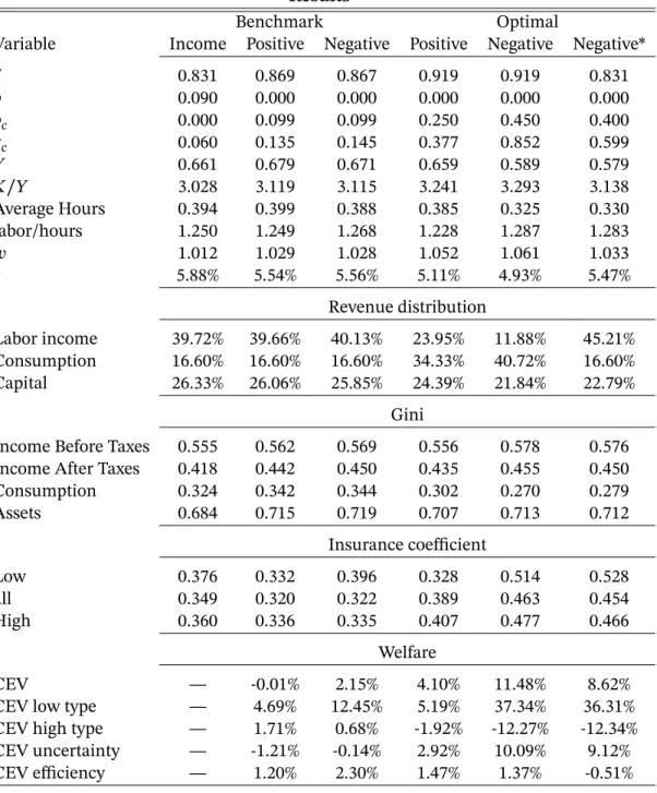
dis-played in Table2. The first four lines in the table display the values for the policy parame-ters at each alternative tax system. In the next six lines the findings for aggregate variables are reported. Next, the revenue distribution block, explains the relative importance of each tax base. The consequence of each system for consumption smoothing is accounted for by the next two blocks. First, the Gini block displays this representative cross-sectional inequality statistic for income before and after taxes, assets and consumption. In the fol-lowing block the insurance coefficient measures how consumption responds to variations in each agent’s productivity changes. It requires longitudinal information.
The first column displays all the relevant statistics for the benchmark allocation. In the second we consider use the same progressivity parameter from the benchmark system but let the progressivity apply to consumption taxes, instead. The level parameter is adjusted to keep tax revenues at the benchmark level.
Hours are slightly increased in benchmark with consumption taxes relative to bench-mark, but there is also a 5% wage increase which indicates that simply moving to progres-sive consumption taxes has a small negative impact on hours.
The large change in the capital stock that arises by simply moving to consumption taxes raises the question of what features matter for our results. We expect to see an important impact on savings; for the preference specification of Section1the coefficient of relative prudence would be increased by 50% with the optimal progressive consumption taxes. Still, the move to a consumption tax cannot be just assumed to be inconsequential in the pres-ence of a warm glow motive for asset accumulation. The findings in a revenue preserving reform displayed in Table5provides further hints to the importance of this channel.
3.1 Optimal Tax Systems
If both distribution and insurance matter, then any tax system trades-off improvements in these two dimensions with potential inefficiencies due to the distortions generated by taxation. The first important thing to notice about the current (benchmark) system is that, from a Utilitarian perspective it errs in the direction of sacrificing too little efficiency and promoting too little redistribution/insurance. This is made clear by our findings regarding the optimal labor income tax schedule. Indeed, if we compare the allocation resulting from optimal labor income taxes with the benchmark allocation we find the efficiency CEV to be 4.02% lower which is more than compensated by a 6.49% increase in the gains from better smoothing as captured by the CEV uncertainty statistics.15
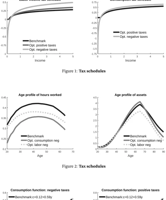
Such a perspective is an important one to bear in mind if we are to understand the results that follow. In our heuristic account of the forces at play, we have emphasized the efficiency gains from moving to a progressive consumption taxes based system. Yet, as one can see, the bulk of the welfare gains, 11.10%, for the optimal consumption tax system are found in the CEV uncertainty statistics. The efficiency gains are explored by the optimal system to provide better insurance and redistribution. Indeed, reinforcing the evaluation above is the labor/hour ratio that compares productivity adjusted hours with total hours: for all but the unrestricted consumption taxes case, the ratio is reduced when compared to the benchmark: the current system provides too little insurance/redistribution for the amount of inefficiencies it creates. To understand how these changes are induced by policy one has to consider the top four rows in Table2. Progressivity increases from 0.090 in the benchmark to 0.220 when we move to optimal labor income taxes (0.130, if taxes are restricted to be non-negative). These numbers are even larger for the case of consumption taxes. Figure3displays the static budget set generated by each tax schedule. It is interesting to note that the benchmark schedule is very close to the optimum if progressivity applies to labor income and taxes are restricted to be non-negative.
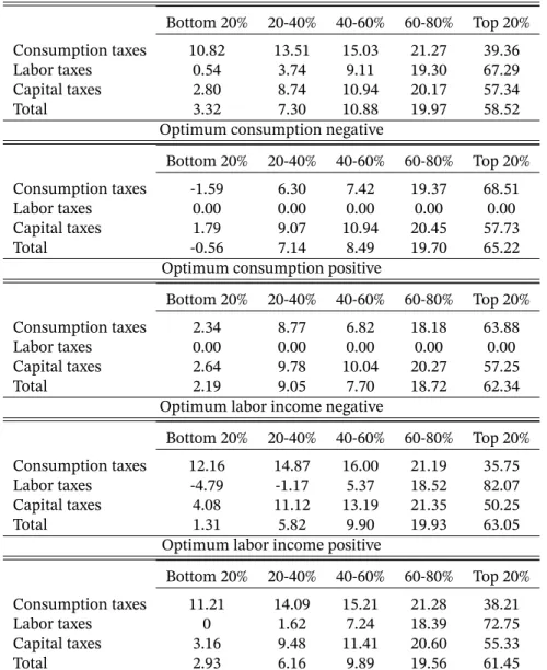
Figure3is very useful if our goal is to compare between systems that share the same tax base. Not so much to compare progressivity across systems that differ with regards to the base since not all earnings are consumed along the life-cycle. This is why we have displayed the budget sets associated with the different tax bases in different panels. To compare across bases we shall now examine progressivity by means of the fraction of revenues raised from each earnings quintile. This approach addresses the aforementioned concerns at the cost of focusing on endogenous objects.
In our main experiment we completely eliminate labor income taxes which leads to
15
Another sign that it is not though efficiency gains that the allocation is improved is the slight reduction in the labor/hours statistics. The tax system is discouraging effort from those with higher productivity more at the optimum than at the benchmark.
a large increase in revenues raised through consumption taxes.16 Progressivity in con-sumption taxes is apparent in Table4, where we measure taxes paid against labor earnings. Interestingly, the most progressive system under this metric is exactly the one with unre-stricted progressive consumption tax schedule. This is all the more significant once one notes that the table displays revenues against income which is not too highly correlated with consumption under this schedule – see Figure3. When unrestricted income taxes are used that we see a highly progressive income tax schedule – in particular note that the four lowest deciles in the income distribution pay negative taxes on average – which might lead us to expect overall progressivity to be at its maximum. However, because we keep capital income tax rates fixed and wealth becomes more concentrated, the unrestricted consump-tion tax system ends up being even more progressive despite the fact that capital income taxes now play a lesser role due to a reduction in the return to capital.
The large welfare gains associated with the reform are, therefore, in a great part due to better consumption smoothing, both in the form of better distribution (of consumption) and more insurance. The improvement in insurance is displayed in the last three rows of Table2. Insurance is higher in all reforms, but the highest improvement occurs when we use the unrestricted progressive consumption schedule. In this case 𝜙 increases from 0.349 in the benchmark to 0.474 at the optimum. For this system, insurance is best for the low type agents. The combined effect of better insurance and distribution induced by progressive consumption schedules is captured by a substantially lower consumption Gini, despite the fact that the same system induces the largest after tax income Gini and largest wealth Gini of all systems. These effects are, perhaps, better illustrated by regressing consumption against income. While the coefficient hovers around .6 whenever income taxes are used, and goes down to around 0.3 when progressive consumption taxes are used, instead.
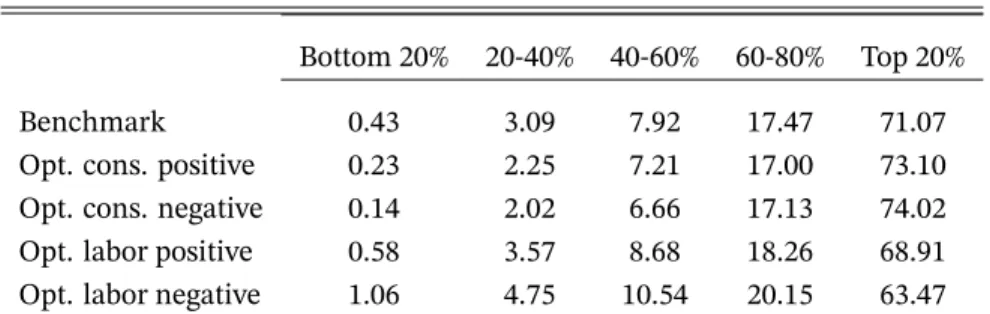
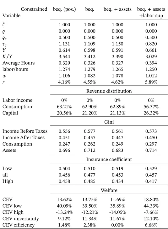
Table3provides further details regarding wealth distribution. The most egalitarian wealth distribution is attained with the unrestricted progressive income tax schedule. In contrast, progressive consumption taxes worsens the wealth distribution even when com-pared to the benchmark. It is in fact possible to check that the normalized wealth dis-tribution associated with the unrestricted optimal consumption tax is dominated in the second order stochastic dominance sense by the benchmark distribution which is, in turn, dominated by the distribution induced by the unrestricted labor income tax. Hence, if the likelihood of fundamental tax reform depends on these currently hotly debated statistics we have only reasons to be pessimistic. Ironically, if a specific group were to oppose the reform, it should be the high productivity group, which would have a substantial welfare loss – 𝐶𝐸𝑉 = −12.70% –, which under a utilitarian metric is more than compensated by
16
the extraordinary gains – 𝐶𝐸𝑉 = 40.34% – obtained by the lowest productivity agents in society.
Beyond the impact on redistribution/insurance this fundamental tax reform leads to important changes in aggregate variables. GDP is almost 10% lower than the benchmark in the allocation induced by the optimal unrestricted progressive consumption taxes despite an increase in the capital income ratio increases by more than 13%. Of course once one accounts for the drop in GDP, then one can see that the capital stock has increased but only by 4%, and that the biggest chunk in the GDP change is explained by a reduction in hours of more than 18%. The large increase in progressivity highlighted in Figure3which still matters from a life-cycle perspective – recall the presentation in Section1– can partly explain this finding. Further evidence on this regard is provided by the fact that an even larger drop in GDP occurs when unrestricted labor income taxes are used. Interestingly, the decline in hours in this case is slightly larger than the one for optimal positive progressive consumption taxes which has similar progressivity – see Figure3.
Most important for our analysis, however, is how hours adjust along the life-cycle, our original motivation for studying this reform. In this case, Figure2makes it plain that while the increase in progressivity that characterize optimal labor income taxes makes hours less responsive to changes in productivity, the move to optimal taxes make them substantially more responsive.
4
Robustness
The move to a system based on progressive consumption taxes has the potential to generate very large welfare gains. Our baseline model is in most aspects canonical. Yet, one feature which may raise some concern is the direct impact of wealth on utility as captured by the warm glow bequest motive.
We have used a specialized version of warm glow motives in which it is only the amount bequeathed that matters for the agent. Consumption taxes change the relative price of consumption with respect to wealth, thus increasing the incentives for wealth accumula-tion. Beyond this, the presence of a warm glow motive raises some important issues for normative analysis. As explained by Kopczuk (2013), under this assumption about be-quest motives welfare improvements are possible by simply taxing bebe-quest and returning to the agents. We eliminate this latter source of spurious gains by not including the util-ity associated with the warm glow term in the welfare evaluation, but we cannot ignore the fact that our specification has important consequences for choices that are not as well settled as other aspects of our model. At issue is the fact that most studies focus on the bequest or wealth taxation. We are not aware of any study directly aimed at assessing the
consequences of consumption taxes on bequests.17 Hence, to assess the robustness of our findings we consider different variations of our experiments that focus on the impact of consumption taxes on welfare accumulation.
First, we restrict the amount of revenues that can be raised by consumption taxes. Sec-ond, we modify preferences to allow the bequest motive to depend on the present value of consumption that wealth can purchase instead of wealth itself. Third, we eliminate the impact of tax changes on savings that arise from the warm glow motive by holding fixed the benchmark policy functions. Finally, we shut down all general equilibrium effects on prices.
4.1 Restricting the role of Consumption Taxes
For the first set of robustness checks we restrict the amount of taxes raised through con-sumption taxes. Our findings are summarized in Table5.
We start by repeating the exercise from Section3in which we use the benchmark labor income tax schedule and progressivity, but now we require the total amount of revenues to be raised via consumption taxes to be held constant at 16.60% of total revenues. CEV drops from 5.27% to ’only’ 2.15%.18 Despite the fact that revenues raised from consumption taxes are held fixed the capital/income ratio still increases by almost 3%. Wealth is disproportion-ately accumulated by those with higher income, hence progressivity and not only the level of consumption taxes matter for capital accumulation. All consumption smoothing statis-tics – Consumption Gini and Insurance Coefficient – decline with this reform. In a sense it is unfair to say that progressivity is preserved with this reform. Since not all earnings are consumed, progressivity applies to a smaller share of agents’ lifetime income. Moreover, because the rich save more, progressivity is significantly reduced. So these results really apply to a policy that is very far from the optimum.
If we maintain the restriction that revenues raised by consumption taxes cannot exceed 16.60%, but allow progressivity to be optimally chosen, then welfare gains are again very high, 𝐶𝐸𝑉 = 8.62%. These welfare gains arise despite a 9% reduction in the capital stock! The emphasis is important. If we restrict consumption tax revenues, we attain lower, albeit still very large, welfare gains in the steady state comparison. Note that this lower gain is accompanied by a large decline in capital stock, whereas in our baseline exercise the capital
17
Diamond(2006);Kopczuk(2013) both comment on the normative shortcomings of relying on a reduced form motive. Because we do not know the underlying reasons why people hold on to wealth in ways that cannot be accounted for by pure life-cycle or pure altruistic motives, we have no a priori views on how different tax schemes should affect choices. Most studies have focused on how bequests respond to estate taxes. Yet, without a micro-foundation for the reduced form it is not clear what these findings have to say about behavioral responses to consumption taxes.
18To put in perspective, recent work byKapička(2020) finds a maximum of 2.98% gain from a fundamental tax reform which introduces history dependence on labor income taxes.
stock slightly increases. The large drop in the capital sock suggests very large additional welfare gains if the transition is taken into account.
Next, we fix the level term, 𝜁, in the labor income schedule at the value that preserves average income taxes at the benchmark. We then follow with the same procedure. We find that welfare gains remain very high, 𝐶𝐸𝑉 = 11.48%, which are however 15% lower than the welfare gains obtained in our main exercise, 𝐶𝐸𝑉 = 13.34%. The lower welfare gains occur with a stock of capital that is 4% lower than the one in our baseline reform.
A more relevant drop, more than 50%, would occur if consumption taxes were con-strained to be non-negative. It is not hard to understand why. When taxes cannot be nega-tive, the scope for progressivity for a given revenue requirement is reduced. Income taxes, by further reducing the revenue requirements lead to lower progressivity in consumption taxes. With unrestricted consumption taxes this effect is avoided and progressivity is only slightly lower than in our main policy reform.
With regards to the impact on aggregate variables, the increase in the capital/income ratio is only 2∕3 of the one which occurs in our main policy reform. This leads to a slightly larger drop in GDP – −11% against −10% – despite a slightly smaller reduction in hours −17% against −18%. Small differences in insurance and consumption Gini helps explain why welfare gains are smaller in this case. It is interesting to note how the use of income taxes, by reducing the scope for progressivity of restricted consumption taxes, worsens their consumption smoothing role. In our main policy, reform the largest reduction in the con-sumption Gini occurs when taxes are restricted to be non-negative. When labor income taxes are required to be used the Gini coefficient is raised from 0.225 to 0.302, which ex-plains the bulk of welfare losses.
All in all, requiring some of the revenue to be raised by income taxes lowers welfare gains both through the reduced progressivity that the characterizes the optimal reform in this case and through lower savings that are partially explained by these changes in progressivity, but possibly also by the differences in impact through the warm glow motive.
4.2 The bequest motive
Kopczuk (2013), emphasizes the importance of how one models the worm glow motive for the behavioral consequences of estate taxation. In particular, is it wealth bequeathed or is it wealth inherited that is valued by individuals? Although we do not consider es-tate taxation, an analogous issue arises regarding the amount of consumption that wealth affords.
Hence, to further assess the importance of our chosen warm glow specification, we assume that agents are interested in how much their inheritance is translated into
con-sumption for their descendants. Formally, we modify (15) to account for taxes using 𝜈(𝑎) = 𝜂1(1 +𝑎 − (1 + 𝑟)𝑇(𝑟𝑎)∕𝑟 𝜂2 ) (1−𝛾𝑐) , (15)
where 𝑇(⋅) is given by equation6. Our findings are summarized in Table6.
If agents are concerned with the consumption equivalent of their wealth instead of wealth per se, this reduces the reform’s impact on capital accumulation with a drop of four percentage points in the capital/income ratio, which is very similar to what we found in the alternative policy reform. Welfare gains are lower, but still substantial – 𝐶𝐸𝑉 = 10.95%.
While difference in preferences directly explain some of the changes, a possible indirect effect through a different choice of progressivity cannot, in principle, be ignored. Yet, what we see is a very mild decrease in progressivity. This is also reflected in similar values for the consumption Gini and the insurance coefficients. A larger drop in GDP, therefore, seems to account for most of the difference in welfare gains.
4.3 Constraining Agents’ Choices
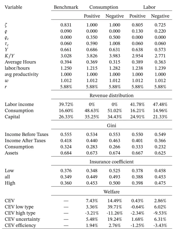
For the next series of robustness we consider some restricted choices that agents can make. Table7displays our main findings.
First, we borrow the policy function from the benchmark, 𝑑𝑎,𝑡(⋅) and generate an asset
accumulation path from 𝑎′ = 𝑑𝑎,𝑡(𝜔), but allow the agents to re-optimize by choosing an
adjustment, ̂𝑎′, which, however, does not take into account the warm glow motive for asset accumulation. In the first column of Table7we assume that only upward adjustments, ̂𝑎′ are possible. Second, we allow arbitrary adjustments that allow ̂𝑎′< 0 but respect ̂𝑎′+𝑎′≥ 0. The most striking aspect about this latter case is how similar the findings are when compared to our baseline findings for unrestricted consumption taxes in Table2. Welfare gains are slightly larger than in our baseline reform. The capital stock is about the same highlighting the fact that the most relevant impacts of our reform cannot be accounted for by the presence of a warm glow motive. Third, we consider the case in which no capital accumulation adjustments are allowed. This is slightly different from allowing agents to solve in every period and in every state of nature a static labor supply problem where the budget constraint is ̂𝑐 ≤ 𝑛𝑤 + 𝐵 for 𝐵 = [1 + 𝑟]𝑎 − 𝑎′, the benchmark asset process. If this was the case agents which were not constrained at the benchmark would respond less to the reform since it would not be the Frisch elasticity but the Marshallian elasticity that would determine the labor supply responses. Here, however, it is the policy function that is borrowed from the baseline exercise; it does not respond to the contemporaneous choice of effort.