Water distribution network reliability: are
surrogate measures reliable?
J. Muranho
1,5*, J. Sousa
2,5, A. Sá Marques
3,5and R. Gomes
4,5 1 University of Beira Interior, Department of Computer Science, Covilhã, Portugal 2 Polytechnic Institute of Coimbra, Department of Civil Engineering, Coimbra, Portugal3 University of Coimbra, Department of Civil Engineering, Coimbra, Portugal 4 Polytechnic Institute of Leiria, School of Technology and Management, Leiria, Portugal 5 INESC – Institute for Systems Engineering and Computers, FCTUC, Coimbra, Portugal
[email protected], [email protected], [email protected], [email protected]
Abstract
Water distribution networks (WDNs) must be reliable infrastructures since they provide an essential service to society. Reliability assessment is a complex task and involves various aspects: mechanical, hydraulic, water quality, water safety, among others. This paper focuses on the hydraulic reliability. Hydraulic reliability is computationally hard to measure directly, therefore researchers came up with surrogate measures, like the resilience index, the modified resilience index, the flow entropy or the diameter-sensitive flow entropy, that are simple and fast to compute. But, are these surrogate measures reliable to be used in the design of WDNs?
This paper proposes a new reliability index based on the surplus flow available on each node to mitigate the effects of a pipe failure. To illustrate the applicability of this new index, a WDN example is optimally designed using a simulated annealing algorithm. Results show that the solutions based on the flow entropy or on the proposed index are more reliable than the others, and, also, the maximization of the other reliability indexes gives only a residual contribution to the global reliability (or even no contribution at all).
1 Introduction
Water distribution systems provide an essential service to society. This kind of infrastructures involves huge investments, so it is necessary to optimize their costs in the design phase, trying to identify solutions that provide good service levels at the lowest cost. However, these two criteria (cost minimization and increased reliability) are conflicting, that is, more reliability implies higher cost and
* Corresponding author.
Engineering
EPiC Series in Engineering
Volume 3, 2018, Pages 1470–1477 HIC 2018. 13th International Conference on Hydroinformatics
the minimum cost solution correspond to low reliability. Given this scenario, designers should seek solutions corresponding to good trade-offs between both criteria.
The least cost design of a WDN is a long-time study problem for the scientific community. Several approaches have been proposed based on different methodologies, from traditional optimization methods, such as linear programming (Alperovits & Shamir, 1997), non-linear programming (Fijiwara & Khang, 1990), and dynamic programming (Liang, 1971), to modern heuristics, much of them inspired on nature processes, such as simulated annealing (Cunha & Sousa, 1999), genetic algorithms (Savic & Walters, 1997), ant colony (Maier et al., 2003), tabu search (Cunha & Ribeiro, 2004), among others. However, since cost minimization tends to eliminate redundancies, this type of approaches generally leads to solutions of reduced reliability.
The WDN reliability refers to the ability to satisfy the required consumptions with enough pressure. The ideal would be achieving reasonable service levels even when facing critical scenarios. However, reaching this would imply unbearable funds. So, the question arises: to what extent will it be feasible to increase investment to reduce risk? On the other hand, the WDN reliability is not easy to assess. One way would be to simulate all potential critical scenarios and, based on the results, compute the level of reliability. However, such kind of procedure is computationally unacceptable, and this gave rise to the use of surrogate measures of reliability. These indirect measures have some weaknesses, but their simplicity and computation speed make them quite attractive. However, are they reliable to be used in the design of water distribution networks?
In the next section, after a brief review of common surrogate measures, a new one is introduced. In the methodology section, these surrogate measures (reliability indexes) are used to build an optimization model that is solved with a simulated annealing algorithm to identify the most reliable solution subject to a maximum budget. The methodology is implemented on WaterNetGen (Muranho et al., 2012, 2014) ─ an EPANET (Rossman, 2000) extension. The case study section presents a comparison of the reliability indexes performances, and some pros and cons are highlighted. The conclusion section draws some conclusions.
2 Reliability indexes – a brief review
In the context of WDN design, reliability has traditionally been achieved through the application of some empirical rules, namely: including redundant pipes to form loops, assign pipe diameters greater than the minimum required diameter and maintain some equilibrium on the diameters within each loop. In the context of optimal design, several approaches have emerged, resulting in a set of methodologies whose objective is to obtain solutions that represent good trade-offs between economy and reliability.
2.1 Entropy and diameter-sensitive entropy
The network reliability quantification based on the entropy concept lay on the following principles: it is desired to have more than one pipe incident to each node (topologic condition) and the incident pipes node must have similar flows (capacity condition). This metric has been proposed by Awumah et
al. (1991). Afterward, Tanyimboh & Templeman (1993) proposed a new expression to compute flow
entropy, which, lately, has been mathematically operated by Walters (1995) to get the following expression: 0 0 1 0 0 =
=
+
N ij ij n n ij TF nQ
Q
QS
QS
E
-
ln
ln
K
QT
QT
QT
QT
(1)
where E is the flow entropy, K is a positive constant, N is the number of network junctions, QT0 is
of network flows, and Qij is the external inflow of node j (i = 0, j = 0), or the external outflow of node
j (i ≠ 0, j = 0), or the flow from node i to node j (i ≠ 0, j ≠ 0).
This metric to compute WDN reliability has two appealing features: it is easy to compute; and, can easily be inserted on optimization models (maximization of flow entropy). However, it is important to note that pipe diameters are not considered, which may lead to solutions with balanced flow rates but with a large disproportion of diameters incident to the same node, which in no way contributes to the network reliability. Trying to avoid this drawback, Liu et al. (2014) proposed a new way to compute the flow entropy, including, although indirectly through the flow velocity, the pipe diameters:
1 0 0 0
1
=
=
+
i N j j i i ij ij i j NR i i i i ND ij i iQ
Q
Q
Q
q
q
E
C
-
ln
-
QT
ln
ln
K
QT
QT
QT
QT
QT
V
QT
QT
(2)
where Qj is the outflow of tank j, NR is the number of tanks, QTi is the inflow to node i, Qi is the
consumption at node i, NDi is the number of pipes leaving node i, C is an arbitrary velocity constant
(for example, 1 m/s), Vij is the flow velocity in pipe ij, and qij is the flow in pipe ij.
However, the correction introduced only affects outflows, which does not seem to make much sense, since the objective is to assure the nodal supply, and this improves with uniformization of the diameters incident to the nodes not with those coming out from the nodes.
2.2 Resilience and net resilience
The resilience index (Ir), proposed by Todini (2000), is based on the principle that the greater the
surplus pressure (difference between observed and required pressures) the better the response of the network to critical scenarios (greater resilience). Thus, the resilience index turns out to represent the quotient between the surplus of the power available in the network (consumptions times pressure slacks) and the surplus of power supplied to the network (power supplied by tanks and pumps minus the power corresponding to the demand satisfaction at the required minimum pressure):
(
)
N * i i i i r NR NP N * j j K K i i j k iQ
H - H
I
Q
H
Q
H -
Q
H
= = = =
=
+
1 1 1 1(3)
where Hi is the head at node i, Hi* is the head at minimum delivery pressure at node i, Hj is the head
at tank j, NP is the number of pumps, Qk is the flow at pump k, Hk is the power introduced into the
network by pump k.
In short, the resilience index weighs the negative effect of the energy losses suffered along the water paths (for example, in a WDN without energy losses the resilience index would be maximum, that is, equal to 1.0). But the fact that it does not consider the network topology, or the pipe capacity, weakens it as a surrogate measure of the network reliability. To overcome, or reduce, this drawback, Prasad & Park (2003) changed the original expression and introduced the uniformization coefficients of the diameters, resulting in the net resilience index (In):
(
)
, where
i NC N * j i i i i j i n NR NP N i * i j j j K K i i j k iD
C
Q
H - H
I
C
NC
máx D
(
Q
H
Q
H -
Q
H )
= = = = =
=
=
+
1 1 1 1 1(4)
where Ci is the diameter uniformity coefficient for node i, NCi is the number of pipes connected to
However, this modification does not seem to be the ideal way to overcome the drawback of the original formula, since the reliability of a WDN is related to the diameters uniformity within each loop and not to the uniformity of diameters of the pipes connected to a node.
2.3 The WNG Index
Considering the issues about the above metrics, a new index, here called WNG Index (WaterNetGen Index), was conceived to estimate the capacity of the network to supply the required demand in the presence of a pipe failure.
For each pipe (j) the surplus flow (QSPj) is the difference between its maximum flow capacity,
computed with a maximum allowed flow velocity (here considered as 1.0 m/s), and its current flow (set to zero if this difference is negative). The idea is to use the pipe surplus flow to mitigate the effects of other pipe failures (connected to its downstream node).
QAj is defined as the difference between the current flow in pipe j (qj), in normal conditions scenario,
and the sum of the surplus flows from all the other pipes supplying the same downstream node (it represents the flow portion of pipe j that can’t be compensated by the other pipes). IAj is an estimate for
the WDN demand satisfaction ratio (DSR) when pipe j is out of service. Let NPPj be the number of
inflow pipes at the downstream node of pipe j, NPP the number of pipes in the WDN, and, as before,
QT0 is the network total consumption, the final index is defined as:
where
and
j NPP i T j i index j j j i i T i jI A
NPP
Q
QA
WNG
,
IA
QA
q
QSP
NPP
Q
= = −
=
1=
0=
−
1 00
(5)
3 Methodology
To assess the effectiveness of the above indirect measures, these metrics were implemented in WaterNetGen. The software was adapted to allow i) the evaluation of reliability indexes; and ii) optimize the design considering the maximization of any reliability index subject to a maximum budget. In the first case, it is enough to simulate the network model to obtain the required hydraulic data (flow rates, velocities, heads, and pressures) and then compute the reliability indexes. For designing, it is necessary to choose the reliability index for the objective function and the maximum allowable cost limit (budget), which can be a fixed value or a percentage of the cost of the current solution. The optimal design problem is solved using a Simulated Annealing algorithm (Kirkpatrick et al., 1983).
The testbed tries to answer the question: to what extent the WDN is able to satisfy the required water demand, even in the scenarios of breaking one pipe? The pipe break scenarios are studied considering that the pipe is out of service (closed). The simulation has been executed by the WaterNetGen’s pressure-driven simulation module, so the ratio of the required demand that is effectively satisfied can be computed. To assess the global reliability of the WDN, all possibilities of only one closed pipe are simulated (as many simulations as the number of pipes). In each simulation, the DSR is computed and the global reliability of the WDN is here given by the average of these ratios.
4 Case study
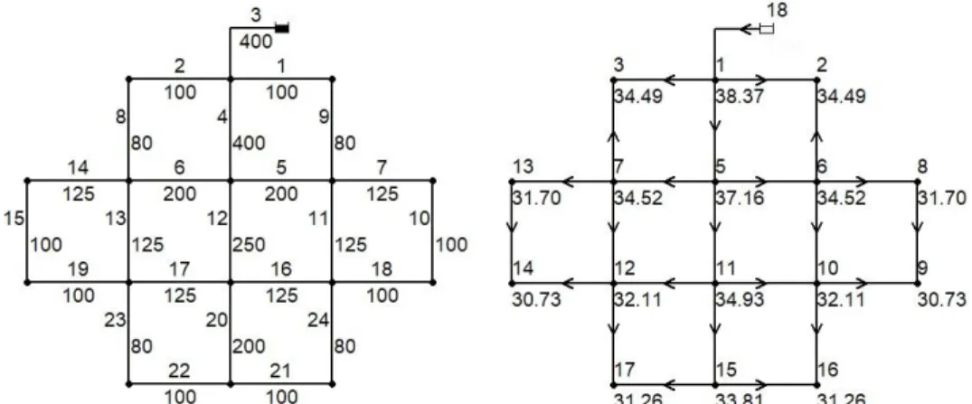
The WDN used in the case study has 1 tank (elevation 40 m), 16 junctions (elevation 0 m), 24 pipes (length 1,000 m) – Figure 1. The network is supposed to supply 20,000 inhabitants, with a per capita consumption of 150 L/day, with an instantaneous peak factor of 2.5 and 20% of water losses. Thus, for
sizing purposes, the network must supply 93.750 L/s with a minimum service pressure of 30.592 m. Table 1 shows the pipe catalogue for the sizing process. In a first phase, the optimization process is driven to find the least cost solution that fulfils the minimum required pressure at all nodes, with a minimum diameters constraint of 80 mm, which corresponds to a total cost of 1,614,670 (€). The network layout is symmetric, so the least cost solution also has symmetric diameters (Figure 1).
The procedure implemented to assess the global reliability (simulations with all pipes out of service, one at a time) gives a final value of 0.911 – Table 2. That is, even in the case of a one pipe break scenario, on average, it is possible to satisfy about 90% of the required demand, with DSR [0,1].
The lowest reliability value is zero and corresponds to the simulation with pipe 3 (the pipe connected to the tank) out of service, which is obvious, because in this case there is no possibility of supply any water. The second and third lowest value (0.255, and 0.881) corresponds to pipes 4, and 12, respectively, which are also structural pipes in this network, so it is not a surprise. All other values are higher than
Diameter (mm) Cost (€) Diameter (mm) Cost (€)
60 33.8 250 118.8 80 36.7 300 145.7 100 43.9 350 180.6 125 53.9 400 205.7 150 69.7 450 244.2 200 87.7 500 282.6
Table 1: Pipe catalogue (Ductile iron, Hazen-Williams roughness, 120)
Pipe DSR Pipe DSR Pipe DSR Pipe DSR
1 0.995 7 0.982 13 0.995 19 0.996 2 0.995 8 1.000 14 0.982 20 0.949 3 0.000 9 1.000 15 0.998 21 0.993 4 0.255 10 0.998 16 0.993 22 0.993 5 0.936 11 0.995 17 0.993 23 0.999 6 0.936 12 0.881 18 0.996 24 0.999
Table 2: Demand satisfaction ratios (DSR’s) for the least cost solution (global reliability= 0.911). Figure 1: Water distribution network layout, with pipe diameters (left) and nodal pressures (right) for the least cost solution.
0.9, with some reaching the maximum value, so, even with these pipes out-of-service (8, and 9) the network would be able to satisfy the required demand. This situation is also easy to explain, since these are small pipes (minimum allowed diameter) with minimum impact in the overall performance of the WDN.
The next phase is to maximize the reliability indexes, subject to a cost that does not exceed the minimum cost by more than 10%, that is the cost must be less than 1,776,137 (€). These second phase takes as input the least cost solution found in the previous phase. Figure 2 illustrates the flow distribution for the least cost and the optimal entropy solutions. This figure clearly shows a better (uniformized) distribution of flows for the entropy-based solution ─ as expected.
Table 3 shows the network DSR’s for the maximum flow entropy solution, where an increase of the DSR from scenarios of breaks in pipes 4 and 12 can be observed. The reason for this improvement, as illustrated in Figure 2, is the more uniform distribution of flows in the network.
Table 4 shows the reliability indexes for each solution. It can be seen that maximizing one index does not necessarily imply the improvement of the others. The analysis of the global reliability values considering the optimal solutions seems leading to the conclusion that the maximization of the diameter-sensitive entropy, resilience index and network resilience index, besides being more expensive, has only a residual contribution to the global reliability of the network, or even no contribution at all, when compared to the least cost solution – which confirms the concerns previously pointed out in section 2. Apparently, only the flow entropy and the WNG Index contributed to the global reliability. But even these metrics show some inconsistences. For example, the flow entropy values 3.0106 (least cost) and 2.9882 (net resilience) corresponds to global reliability values of 0.911 and 0.914, respectively. That is, a lower value for the flow entropy corresponds to a greater value of the global reliability. The same behaviour can be observed for the WNG Index.
Figure 2: Network flows for the least cost (left) and maximum flow entropy solutions (right).
Pipe DSR Pipe DSR Pipe DSR Pipe DSR
1 0.989 7 0.985 13 0.981 19 0.993 2 0.991 8 0.996 14 0.983 20 0.997 3 0.000 9 0.995 15 0.999 21 0.998 4 0.864 10 0.999 16 1.000 22 1.000 5 0.994 11 0.981 17 1.000 23 0.988 6 0.996 12 0.991 18 0.997 24 0.986
Figure 3 shows that, in fact, only the flow entropy and the WNG Index follow a trend similar to the global reliability, while the diameter sensitive entropy is very inconsistent, and the resilience index and the net resilience depict a random behaviour. It is worthy of note that the WNG Index is normalized, it takes values between 0.0 (no reliability) and 1.0 (full reliability), making the reliability assessment easier (when compared to some of the other indexes).
5 Conclusions
WDN reliability assessment is an important subject in the design of these infrastructures. However, since its full assessment is too complex, it is common to use surrogate measures (reliability indexes) to do it expeditiously. Nevertheless, as these indexes are empirical and do not always consider some aspects that effectively condition the reliability of the WDNs, some caution must be taken in its use. In this work, five reliability indexes (flow entropy, diameter-sensitive entropy, resilience index, network resilience, and a new one) were evaluated for a case study (hypothetical network). It is concluded that the maximization of one index does not necessarily imply the improvement of the others. The analysis of global reliability values (average DSR when one pipe is out of service) for the solutions obtained seems leading to the conclusion that the maximization of some indexes (diameter-sensitive entropy,
Figure 3: Global reliability vs. other reliability indexes. 0.4 0.5 0.6 0.7 0.8 0.9 1.0 1.1 0.910 0.915 0.920 0.925 0.930 0.935 0.940 0.945 0.950 R e li a b il it y In d e x / M a x im u m R e li a b il it y In d e x Global Reliability
Entropy D.S. Entropy Resilience Net Resilience WNG Index Table 4: Comparison of reliability indexes.
Global Entropy D.S. Entropy Resilience Net Resilience WDN Index Reliability
3.0106 5.8392 0.3313 0.2371 0.8803 1 614 670 0.911 Entropy 3.3951 6.4595 0.3626 0.2943 0.8986 1 772 530 0.946 D.S. Entropy 2.9469 10.9989 0.3511 0.2443 0.8749 1 770 780 0.911 Resilience 2.9546 6.5980 0.6150 0.4300 0.8758 1 774 610 0.911 Net Resilience 2.9882 6.4953 0.5978 0.4337 0.8760 1 773 520 0.914 WDN Index 3.2390 6.8524 0.2527 0.1994 0.9035 1 774 550 0.939
Network Realibility Indexes Least Cost Cost (€) M a x im iz e
resilience index and network resilience) has only a residual contribution to the global reliability of the network (or even no contribution at all). Apparently, only the maximization of the flow entropy or the new index (WNG Index) improves the overall network reliability. Even so, all indexes analyzed show some kind of inconsistence: the global network reliability value is not strictly increasing with the indexes.
The WNG Index is a normalized metric that takes values between 0.0 (no reliability) and 1.0 (full reliability), making the reliability assessment easier (when compared to some of the other indexes).
References
Alperovits, E., Shamir, U. (1997). Design of optimal water distribution systems, Water Resources
Research, 13(6), pp. 885-900.
Awumah, K., Goulter, I., Bhatt, S.K. (1991). Entropy-based redundancy measures in water-distribution networks, Journal of Hydraulic Engineering, ASCE, 117(5), pp. 595-614.
Cunha, M.C., Ribeiro, L. (2004). Tabu Search algorithms for water network optimization, European
Journal of Operational Research, 157(3), pp. 746-758.
Cunha, M.C., Sousa, J. (1999). Water distribution network design optimization: Simulated Annealing approach. J. Water Resources Planning and Management, ASCE, 125(4), pp. 215-221.
Fujiwara, O., Khang, D.B. (1990). A two-phase decomposition method for optimal design of looped water distribution networks, Water Resources Research, 26(4), pp. 539-549.
Kirkpatrick, S., Gelatt, C.D., Vecchi, M.P. (1983). Optimization by simulated annealing, Science, 220(4598), pp. 671-680.
Liang, T. (1971). Design of conduit system by Dynamic Programming, Journal of the Hydraulics
Division, ASCE, 97(3), pp. 383-393.
Liu, H., Savic, D., Kapelan, Z., Zhao, M., Yuan, Y., Zhao, H. (2014). A diameter-sensitive flow entropy method for reliability consideration in water distribution system design, Water Resources
Research, 50, pp. 5597–5610.
Maier, H.R., Simpson, A.R., Zecchin, A.C., Foong, W.K., Phang, K.Y., Seah, H.Y., Tan, C.L. (2003). Ant colony optimization for design of water distribution systems, Journal of Water Resources
Planning and Management, ASCE, 129(3), pp. 200-209.
Muranho, J., Ferreira, A., Sousa, J., Gomes, A., Sá Marques, A. (2012). WaterNetGen – an EPANET extension for automatic water distribution network models generation and pipe sizing, Water Science
& Technology: Water Supply, IWA Publishing, 12(1), pp. 117-123.
Muranho, J., Ferreira, A., Sousa, J., Gomes, A., Sá Marques, A. (2014). Pressure-dependent Demand and Leakage Modelling with an EPANET Extension – WaterNetGen, Procedia Engineering, 89, pp. 632-639.
Prasad, T.D., Sung-Hoon, H., Namsik, P. (2003). Reliability based design of water distribution networks using multiobjective genetic algorithms, KSCE J. of Civil Engineering, 7(3), pp. 351-361.
Rossman, L.A. (2000). EPANET2 User’s Manual, Drinking Water Research Division, Risk Reduction Engineering Laboratory, U.S. Environmental Protection Agency, Cincinnati.
Savic, D.A., Walters, G.A. (1997). Genetic algorithms for least-cost design of water distribution networks, Journal of Water Resources Planning and Management, ASCE, 123(2), pp. 67-77.
Tanyimboh, T.T., Templeman, A.B. (1993). Calculating maximum entropy flows in networks,
Journal of Operational Research Society, 44(4), pp. 383-396.
Todini, E. (2000). Looped water distribution networks design using a resilience index based heuristic approach, Urban Water Journal, 2 (3), pp. 115–122.
Walters, G.A. (1995). Discussion of “Maximum entropy flows in single source networks” from T.T. Tanyimboh and A.B. Templeman, Engineering Optimization, 25, pp. 155-163.