Differential absorption radar techniques: water vapor retrievals

(1)

www.atmos-meas-tech.net/9/2633/2016/ doi:10.5194/amt-9-2633-2016

Differential absorption radar techniques: water vapor retrievals

Luis Millán, Matthew Lebsock, Nathaniel Livesey, and Simone Tanelli

Jet Propulsion Laboratory, California Institute of Technology, Pasadena, California, USA

Correspondence to:Luis Millán ([email protected])

Received: 8 March 2016 – Published in Atmos. Meas. Tech. Discuss.: 22 March 2016 Revised: 26 May 2016 – Accepted: 30 May 2016 – Published: 21 June 2016

Abstract.Two radar pulses sent at different frequencies near the 183 GHz water vapor line can be used to determine total column water vapor and water vapor profiles (within clouds or precipitation) exploiting the differential absorption on and off the line. We assess these water vapor measurements by applying a radar instrument simulator to CloudSat pixels and then running end retrieval simulations. These end-to-end retrievals enable us to fully characterize not only the ex-pected precision but also their potential biases, allowing us to select radar tones that maximize the water vapor signal minimizing potential errors due to spectral variations in the target extinction properties. A hypothetical CloudSat-like in-strument with 500 m by ∼1 km vertical and horizontal res-olution and a minimum detectable signal and radar preci-sion of −30 and 0.16 dBZ, respectively, can estimate total column water vapor with an expected precision of around 0.03 cm, with potential biases smaller than 0.26 cm most of the time, even under rainy conditions. The expected preci-sion for water vapor profiles was found to be around 89 % on average, with potential biases smaller than 77 % most of the time when the profile is being retrieved close to surface but smaller than 38 % above 3 km. By using either horizontal or vertical averaging, the precision will improve vastly, with the measurements still retaining a considerably high vertical and/or horizontal resolution.

1 Introduction

The WMO (2014) statement of guidance for global numeri-cal weather prediction concluded that one of the critinumeri-cal at-mospheric variables that are not adequately measured by cur-rent or planned systems is humidity; in particular, profiles with adequate vertical resolution in cloudy areas were rec-ommended (Anderson, 2014). Due to its importance, sev-eral spaceborne methods have been used to observe

atmo-spheric water vapor, such as passive near-infrared or mi-crowave imaging, passive infrared or mimi-crowave sounding, and radio occultation techniques. Most of these techniques have been shown to improve weather forecasting perfor-mance once assimilated (Anderson, 2007) and are opera-tionally used, but each has limitations. For example, infrared and microwave sounders have broad weighting functions near the Earth’s surface, which considerably limit their ver-tical resolution. Near-infrared and microwave imaging can only provide column water vapor, and hence they do not pro-vide any information on its vertical distribution. Addition-ally, near-infrared and infrared techniques cannot penetrate cloudy scenes. Lastly, even though radio-occultation tech-niques are sensitive even to the boundary layer water vapor burden, atmospheric ducting effects associated with the top of the boundary layer limit their accuracy (Ao et al., 2003).

(2)

vapor line using large eddy simulations (LES). These high-resolution LES allowed the assessment of uncertainties due to small-scale heterogeneities within the radar field of view (commonly known as non-uniform beam filling) as well as uncertainties due to the particle size distribution. However they do not provide context on the capabilities of DAR over a wide variety of Earth’s clouds. This global climatological context is best provided by observations. Following Lebsock et al. (2015) the study will focus on the wing of the 183 GHz water vapor line, but we will evaluate the DAR capabilities using global cloud observations from CloudSat (Stephens et al., 2002). The water vapor line at 183 GHz is used rather than the 22 GHz because its attenuation is stronger which provides a greater dynamical range allowing us to explore cloud and rain profiling. We specifically focus on a space-borne observational platform.

A spaceborne implementation of a water vapor DAR would provide observational capabilities that complement existing remote sensing methods. In particular the method specifically samples within the cloudy environment. This could provide much needed observations within the poorly sampled cloudy boundary layer and help constrain the rel-ative humidity in ice clouds. Furthermore, the method can provide high spatial resolution column water vapor in all weather conditions and over all surfaces.

In this study we evaluate the ability of the DAR technique to retrieve water vapor with high vertical and horizontal reso-lutions under cloudy/rainy conditions and we diagnose which radar tones are better suited for sampling different altitude ranges. This paper is organized as follows: the measurement theory is described in Sect. 2, the radiometric model is de-scribed in Sect. 3, total column water vapor retrievals are discussed in Sect. 4, while Sect. 5 explores the profiling ca-pabilities of this technique. Section 6 summarizes the results.

2 Theoretical basis

As shown by Lebsock et al. (2015), the ratio of two radar re-flectivities, neglecting multiple scattering, can be expressed as

Z(ν1, r)

Z(ν2, r) =

ϒ2(ν1, r) η(ν1, r) λ41

ϒ2_(ν

2, r) η(ν2, r) λ42

|K(ν2, r)|2

|K(ν1, r)|2

, (1)

where ν is a radar tone frequency,λ is the wavelength of radiation, andK(ν, r)is the dielectric constant of the target. η(ν, r)represents the hydrometeors backscatter coefficients andϒ2(ν, r)is the two-way transmission along the ranger given by

ϒ2(ν, r)₌exp



−2

r

Z

0

σgas(ν, r)+σPext(ν, r)

dr



, (2)

where σgas(ν, r) represents the gaseous absorption

coeffi-cient and σPext(ν, r) the particulate extinction (the sum of

160 162 164 166 168 170 172 174 176 178 180 182 184 186 188 190 192 194 196 198 200 Frequency [GHz]

-30 -25 -20 -15 -10 -5

[dB]

ϒ2

gas ϒ

2 Pext

η σ0_{- 30}

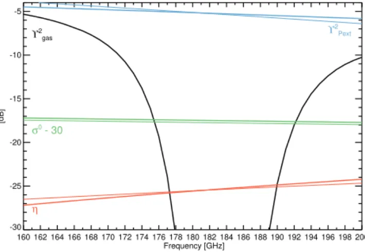
Figure 1.Example of a typical atmospheric transmittance due to

gases (ϒgas2 (ν), black) and hydrometeors (ϒPext2 (ν), blue), as well as the backscatter reflectivity (η(ν), red), and the ocean backscatter (σ₀2(ν)green, offset by 30 dB) for a surface return journey (down-ward atmospheric pass, surface reflection, up(down-ward pass) for a nim-bostratus cloud near the 183 GHz H2O band region. The atmo-spheric profile was taken from CloudSat data as described in Sect. 3. The ocean backscatter corresponds to a surface wind of 3 m s−1and temperature of 28◦C. Note that only the transmittance due to gases shows a significant frequency dependence. Thin lines show the im-pact of assuming a different particle size distribution or a differ-ent surface wind. These lines have been offset to ease comparison against the unperturbed ones.

absorption and scattering) coefficient. Note that in Eq. (1), when the scattering target is the surface rather that hydrom-eteors along the path,η(ν, r)is replaced by the normalized surface cross sectionσ0(ν).

Assuming that these frequencies are chosen close to a strong absorption line, and the frequency dependence of σPext(ν, r), η(ν, r), and σ0(ν) is small relative to that of

σgas(ν, r)(see Fig. 1), Eq. (1) simply becomes

Z(ν1, r)

Z(ν2, r) =

ϒ2(ν1, r)

ϒ2_(ν 2, r)

=exp



−2

r

Z

0

σgas(ν1, r)−σgas(ν2, r)dr 

, (3)

which can be rewritten as Z(ν1, r)

Z(ν2, r)

=exp



−2

r

Z

0

ρ(r)X

i

vi(r)[κi(ν1, r)−κi(ν2, r)] dr 

, (4)

whereρ(r)is the air density and the sum is over all the ab-sorbers with monochromatic absorption coefficientκi(ν, r)

and volume mixing ratiovi(r).

(3)

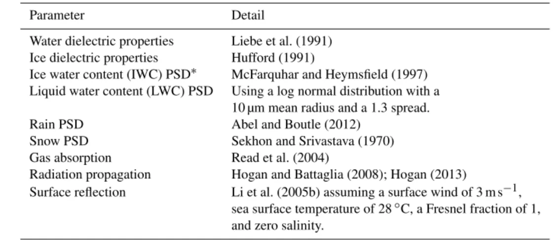
ab-Table 1.Radar model specifics

Parameter Detail

Water dielectric properties Liebe et al. (1991) Ice dielectric properties Hufford (1991)

Ice water content (IWC) PSD∗ McFarquhar and Heymsfield (1997) Liquid water content (LWC) PSD Using a log normal distribution with a

10 µm mean radius and a 1.3 spread.

Rain PSD Abel and Boutle (2012)

Snow PSD Sekhon and Srivastava (1970)

Gas absorption Read et al. (2004)

Radiation propagation Hogan and Battaglia (2008); Hogan (2013)

Surface reflection Li et al. (2005b) assuming a surface wind of 3 m s−1, sea surface temperature of 28◦C, a Fresnel fraction of 1, and zero salinity.

∗particle size distribution.

sorbers (at two close enough frequencies) are similar, leaving mostly the influence of the main absorber. For example, next to the 183 GHz H2O absorption line, Eq. (4) can be

simpli-fied as

Z(ν₁, r)

Z(ν₂, r)

=exp



−2

r

Z

0

ρ(r) vH2O(r)[κH2O(ν1, r)−κH2O(ν2, r)] dr



, (5)

which expressed in decibels relative to Z units (dBZ) and, using the ideal gas law, results in

dBZ(ν1, r)−dBZ(ν2, r) ∝uH2O=

r

Z

0

p(r)

R T (r) vH2O(r)dr,

(6) whereRis the gas constant,pis pressure, andT is tempera-ture.

Equation (6) shows that the difference between two radar tones expressed in dBZ units is proportional to the partial water vapor pathuH2O between the radar and the scattering

target. This means that a range-gated radar may be used to es-timate profiles of water vapor density inside cloudy or rainy profiles assuming a temperature and pressure profile (e.g., from reanalysis fields). Furthermore, this technique may be used to estimate the total column water vapor (CWV) us-ing the surface returns. However, the proportionality given by Eq. (6) assumes that the absorption from other gases as well as the particulate extinction and backscattering coeffi-cient between the two radar tones were similar which might not be true under certain hydrometeor burdens.

In this study, a range-gated radar system is simulated to explore the uncertainties in the estimates of total CWV as well as in the profiles of water vapor inside cloudy and rainy scenarios using a state-of-the-art radar forward model. This

model is not based upon Eq. (6), but rather a more com-plete version of Eq. (1) that also includes multiple scattering. Through this model we assess the impact of spectral variation of the particulate extinction and the backscatter coefficient, the impact due to absorption of other gases, the impact of the temperature and pressure profiles assumed, the impact of the assumed hydrometeor particle size distribution, and the im-pact of the spectroscopy uncertainties, among others (see for example Fig. 1 thin lines).

3 Radiometric model

Radar returns were simulated using the same radiometric model as discussed in Millán et al. (2014). In short, radar re-flectivities were computed using time-dependent two-stream approximation (Hogan and Battaglia, 2008), assuming spher-ical hydrometeors, evaluating the gaseous properties using the clear sky forward model for the EOS Microwave Limb Sounder (Read et al., 2004), and computing the surface re-flection using a quasi-specular scattering model for the ocean surface. See Table 1 for more details. Note that even though all the simulations presented in this study used an ocean backscatter model, typical land surface back scattering coef-ficients are also weakly frequency-dependent, and hence, due to the differential nature of the technique, the results shown here can reasonably be expected to be similar to those found over land.

(4)

Euro-Figure 2.Cross section exemplifying the CloudSat-driven simulations (data from 15 January 2007 over the South Atlantic Ocean).(a) Cloud-Sat radar reflectivity.(b)CloudSat retrieved total (IWC+LWC+rain+snow) hydrometeor water content. Black, green, red and purple lines, respectively, delimit areas where IWC, LWC, rain, and snow were present.(c)ECMWF-aux water vapor.(d)Simulated CloudSat-driven radar reflectivity at 170 GHz.(d)Simulated radar reflectivity difference (177–170 GHz).

pean Centre for Medium-Range Weather Forecasts auxiliary (ECMWF-aux) products (Partain, 2007). The ECMWF-aux data are ECMWF weather analysis outputs interpolated in time and space to the CloudSat measurements. We also use the 2B-CLDCLASS product (Sassen and Wang, 2008) for cloud classification. Furthermore, we assume a radar with the same detectable signal (the radar sensitivity) and the same radar precision as CloudSat’s Cloud Profiling Radar (Tanelli et al., 2008), that is to say−30 and 0.16 dBZ, respectively. We also assume a similar vertical ranging and horizontal sampling resolution: 500 m and around 1 km, respectively. Viewing angles off the nadir, provided by using a scanning radar, are not explored in this study but, apart from the extra attenuation due to the longer paths, they are fundamentally the same as when using the nadir view.

As an example to illustrate the nature of the measurement, Fig. 2 shows a cross section of CloudSat-driven simulations over the South Atlantic Ocean. This cross section consists of 700 CloudSat profiles encompassing high thin cirrus, some liquid clouds, rain, and snow. As shown, the water vapor field not only decreases exponentially with height, it also shows a tongue that increases with height along the track, starting from around 32◦S at 5 km and finishing at around 35.5◦S and 10 km. The impact of this water vapor burden can be

seen in the simulated 170 GHz radar reflectivity subplot; at this frequency, the radar signal has been considerably more attenuated than at 94 GHz (the CloudSat radar tone, which was placed far away from any absorption line). Furthermore, the radar reflectivity difference (177–170 GHz) already dis-plays a resemblance to the water vapor field, for example the influence of the water vapor tongue around 10 km and 34.5◦S can already be seen in the radar reflectivity difference.

(5)

temper-Figure 3.Simulated relationships between surface radar returns and total and partial CWV. Each point represents a CloudSat-driven simula-tion for each of the CloudSat measurements available from 15 January 2007. The total or partial hydrometeor column is color-coded. Dark gray is used for clear sky cases (total hydrometeor column equal to zero). The black line shows the linear regression. The root mean square error (RMSE) displayed is the overall linear regression error for each scenario. The top row shows the relationship between the range-gated radar returns and partial CWV and the bottom row displays the relationship between the surface returns and total CWV.

10 100

[%] 0

2 4 6 8 10 12 14

Altitude [km]

160 GHz

161 GHz 162 GHz 166 GHz 169 GHz

170 GHz 172 GHz

174 GHz 177 GHz 178 GHz

181 GHz

183 GHz

Figure 4.Percentage penetration for frequencies discussed in this

study calculated using CloudSat-driven simulations for 10 days, as-suming a radar sensitivity of₋30 dBZ.

ature and pressure profiles for the same water vapor burden. Under cloudy and rainy scenarios the spread also increases proportionally to the mass of condensate.

The root mean square errors (RMSEs) of these linear fits can be interpreted as the maximum likely precision error

of a water vapor retrieval. The results are promising. They show that even without knowledge of the temperature, pres-sure and hydrometeor burden, partial and total CWV can be constrained to less than 0.5 cm under clear and cloudy sce-narios, and to under 0.7 cm for rainy ones. Note that if the hydrometeor burden is known (for example using the range-gated information from the 160 GHz radar tone), one could subset the data using this ancillary information to constrain the partial and total CWV better.

(6)

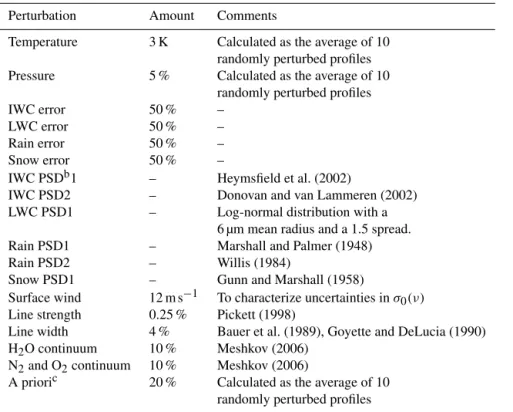
Table 2.Systematic uncertainties perturbationsa.

Perturbation Amount Comments

Temperature 3 K Calculated as the average of 10 randomly perturbed profiles

Pressure 5 % Calculated as the average of 10

randomly perturbed profiles

IWC error 50 % –

LWC error 50 % –

Rain error 50 % –

Snow error 50 % –

IWC PSDb1 – Heymsfield et al. (2002)

IWC PSD2 – Donovan and van Lammeren (2002)

LWC PSD1 – Log-normal distribution with a

6 µm mean radius and a 1.5 spread.

Rain PSD1 – Marshall and Palmer (1948)

Rain PSD2 – Willis (1984)

Snow PSD1 – Gunn and Marshall (1958)

Surface wind 12 m s−1 To characterize uncertainties inσ0(ν) Line strength 0.25 % Pickett (1998)

Line width 4 % Bauer et al. (1989), Goyette and DeLucia (1990) H₂O continuum 10 % Meshkov (2006)

N2and O2continuum 10 % Meshkov (2006)

A prioric 20 % Calculated as the average of 10 randomly perturbed profiles

a_{For the unperturbed characteristics see Table 1.}

b_{Particle size distribution.}

c_{Only applied to profile retrievals.}

few kilometers of the atmosphere. However, notice that the strong surface reflection is detectable 60 % of the time even at 178 GHz. The strength of the surface reflection should enable retrievals of total CWV in a diverse range of environments, even where profiling is not possible.

4 Total column water vapor results

To properly explore the capability of this technique to es-timate total CWV we have performed end-to-end retrievals. The retrieval algorithm used was a linear least-squares fit (see Appendix A for more information) which allow us to quan-tify both the expected precision and the systematic errors of the total CWV estimates using ancillary knowledge of tem-perature, pressure, and the hydrometeor profile. This retrieval does not use any a priori information; that is to say, we do not use any additional information to constrain these retrievals. The expected precision is determined by the random noise in the radar measurements propagated through the retrieval algorithm, while the systematic errors will arise from the un-certainties in the ancillary knowledge used, as well as from the spectroscopy uncertainties. These end-to-end retrievals assume knowledge of the hydrometeors’ vertical distribution. This knowledge is assumed to come from an offline radar tone using CloudSat-like retrievals. The impact of attenua-tion on this radar tone/retrievals is not investigated here.

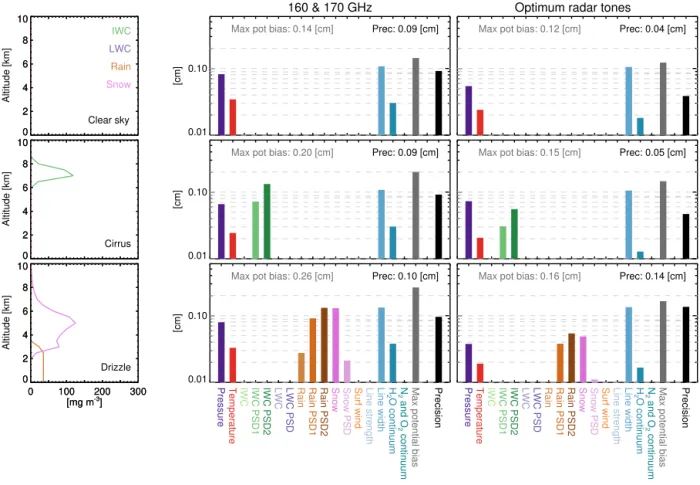
For a given scene, a perturbed set of radar measurements is generated for each systematic uncertainty and run through the retrieval algorithm. Each of the retrieved results is then compared to the retrieved total CWV for an unperturbed run to estimate the impact of such perturbation. A list of the per-turbations used can be found in Table 2. Figure 5 (middle column) shows the systematic error characterization for three different scenarios using the 160 and 170 GHz radar tones.

(7)

Table 3.Optimum radar tones

Scene Radar tones Precisiona Potential biasa Potential biasa

type (GHz) 60 % of the time 80 % of the time

Total CWV (cm)

Clear sky 160, 174 0.01±0.001 0.10 0.14

Cloudy 166, 174 0.01_±0.001 0.10 0.14

Rainyb 169, 172 0.03±0.008 0.18 0.26

Profile H2O (%)

<9 km 178, 183 86_±33 20 26

9–12 km 178, 183 84±77 13 20

6–9 km 178, 181 93_±83 25 37

3–6 km 169, 177 69±63 48 81

1–3 km 162, 172 87_±64 50 78

0–1 km 160, 170 114±77 29 70

a_{Estimates computed using end-to-end retrievals for each of the CloudSat measurements available from 15 January 2007.}

b_{Rain rates lower 10 mm h}−1_.

0 2 4 6 8 10

Altitude [km]

0 2 4 6 8 10

IWC

LWC

Rain

Snow

Clear sky

160 & 170 GHz

0.01

0.10

[cm]

Max pot bias: 0.14 [cm] Prec: 0.09 [cm]

Optimum radar tones

0 2 4 6 8 10

Altitude [km]

0 2 4 6 8 10

Cirrus

0.01

0.10

[cm]

0 100 200 300

[mg m-3_]

0 2 4 6 8 10

Altitude [km]

0 100 200 300

[mg m-3_]

0 2 4 6 8 10

Drizzle

0.01

0.10

[cm]

Pressure Temperature IWC IWC PSD1 IWC PSD2 LWC LWC PSD Rain Rain PSD1 Rain PSD2 Snow Snow PSD Surf wind Line strength Line width H

O

continuum

2

N

and

O

continuum

2

Max potential bias Precision Max pot bias: 0.26 [cm] Prec: 0.10 [cm]

Pressure Temperature IWC IWC PSD1 IWC PSD2 LWC LWC PSD Rain Rain PSD1 Rain PSD2 Snow Snow PSD Surf wind Line strength Line width H_O

continuum

2

N

and

O

continuum

2

Max potential bias Precision Max pot bias: 0.16 [cm] Prec: 0.14 [cm]

Figure 5.Systematic error estimates for total column water vapor retrievals caused by each of the sources described in Table 2 as well as

the precision and maximum potential bias for three different scenarios (clear sky, cirrus, and drizzle). The maximum potential bias is the root-sum-square combination of all the systematic error sources. Left: hydrometeor burden for each of the scenarios; middle: simulations performed using 160 and 170 GHz radar tones; right: simulation using optimum radar tones (see Table 3).

(i.e the attenuation in the on channel) and hence minimize the impact of the random noise. For rainy cases, the radar tones are close to each other (just 3 GHz baseline) to minimize the impact of the uncertainties associated with the hydrometeors. Lastly, the cloudy cases sit in between these two extremes

(8 GHz baseline), trying to minimize both the precision and the systematic errors.

(8)

Clear sky

0.0 0.1 0.2 0.3 Max pot bias [cm] 0.00

0.05 0.10 0.15 0.20 0.25 0.30

Frequency

0.0 0.1 0.2 0.3 0.00

0.05 0.10 0.15 0.20 0.25 0.30

Frequency

Cloudy

0.0 0.1 0.2 0.3 Max pot bias [cm]

Cloudy

0.0 0.1 0.2 0.3

Rainy

0.0 0.3 0.6 0.9 0.0 0.2 0.4 0.6 0.8 1.0

Cumulative frequency

Rainy

0.0 0.3 0.6 0.9 Max pot bias [cm]

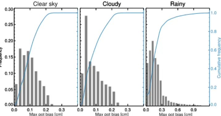
Figure 6.Histogram (gray) and cumulative histogram (blue) of the

maximum potential biases for CloudSat-driven end-to-end total col-umn water vapor retrievals for each of the CloudSat measurements available from 15 January 2007.

column) shows the impact of using the optimized radar tones. Overall, the precision has improved and the maximum poten-tial biases (the root-sum-square combination of all the sys-tematic error sources) have decreased compared to the re-sults using the 160 and 170 GHz radar tones. Observe that for the drizzle case, even though the precision has decreased, the optimum radar tones minimize the total error. In general, the most persistent potential bias is due to the water vapor line width uncertainty, followed by the assumed pressure pro-file. In cloudy and rainy situations this is followed by the hy-drometeor error as well as their corresponding particle size distribution (PSD) uncertainties. Lastly, biases induced by uncertainties in temperature, surface wind, the background atmospheric absorption from O2, N2, and H2O (i.e., the

ab-sorption continuum), as well as the water vapor line strength, are negligible.

To fully test the optimized radar tones, we have run end-to-end retrieval simulations for CloudSat measurements from 15 January 2007 (more than 150 000 pixels). Histograms and cumulative histograms of the maximum potential biases are shown in Fig. 6. Even under rainy conditions the expected precision was found to be 0.03 cm on average, with potential biases smaller than 0.26 cm 80 % of the time. Table 3 lists the precision and potential biases for all weather conditions. This expected precision is half of the Advanced Microwave Scanning Radiometer (AMSR) expected total CWV preci-sion reported by Wentz and Meissner (2000). The greater precision of DAR relative to the passive microwave results from the fact that DAR makes use of the stronger 183 GHz line, whereas passive microwave relies on the 22 GHz line.

Arguably to date, passive microwave instruments have provided the benchmark for CWV measurements. Not only might DAR total CWV have better precision but could also have a considerable better horizontal resolution, i.e., around 1 km rather than the native passive microwave footprint of

∼24 km. Further, DAR total CWV estimates will be avail-able over land and ocean rather that just over the oceans.

5 Profiling capabilities

As with total CWV, we have used end-to-end retrievals to further study the capabilities of this technique to estimate profiles of water vapor under cloudy and rainy scenarios. In this case, we have used an optimal estimation algorithm (Rodgers, 2000). This algorithm uses a priori data to con-strain the retrieval. This additional information acts as an extra set of measurements and the solution can be thought as a weighted average between the measurements and the a priori. The a priori used is the mean profile of 100 adjacent CloudSat ECMWF-aux water vapor values smoothed by a boxcar average of four vertical levels. The uncertainties in this a priori are assumed to be 100 %, allowing the informa-tion to arise mostly from the simulated measurements. See Appendix B for more information.

Figure 7 exemplifies the profiling capabilities of this tech-nique for a raining profile. As shown, different pairs of radar tones can sample different parts of the cloudy/rainy atmo-sphere: tones close to the line center can sample higher alti-tudes, while tones with moderate water vapor absorption can penetrate further into the surface. This can be appreciated in the averaging kernels subplots. These kernels delimitate the region of the atmosphere from which the atmospheric infor-mation is contributing to the retrieved values at a given alti-tude (Rodgers, 2000). Hence, if only two radar tones are go-ing to be used, they will need to be carefully chosen to be able to sample the desired vertical region. In this study, altitudes where the kernel maximum is greater than 0.4 are considered to have retrievals not influenced too much by the a priori and therefore carry useful retrieved information. The expected precision and systematic errors are only shown for those al-titudes. As shown in the last row of Fig. 7, it is possible to sample the entire vertical profile using multiple radar tones. Figure 8 shows the retrieved water vapor profiles over the same cross section displayed in Fig. 2c. As shown, this tech-nique could provide valuable information for studies of water vapor vertical and horizontal distribution in cloudy/rainy ar-eas and as input to weather forecasting models, complement-ing the existcomplement-ing water vapor measurements well. The use of multiple radar tones is analyzed here purely from an infor-mation content point of view with no concern for practical implementation matters.

(9)

0 2 4 6 8 10 12

Altitude [km]

IWC

Snow

Rain

183– 178 GHz

0 2 4 6 8 10 12

Altitude [km]

181– 178 GHz

0 2 4 6 8 10 12

Altitude [km]

177– 169 GHz

0 2 4 6 8 10 12

Altitude [km]

172– 162 GHz

0 2 4 6 8 10 12

Altitude [km]

170– 160 GHz

0 100 200 [mg m-3_] 0

2 4 6 8 10 12

Altitude [km]

0.0 0.4 0.8 Av. kernels

Multi-tones

0.1 1.0 10.0 100.0 Sys. error [%]

Pressure

Temperature

IWC IWC PSD1 IWC PSD2

Rain

Rain PSD1 Rain PSD2 Snow

Snow PSD

Surf wind

Line strength

Line width

H O cont.2

N and O cont.2 2 Apriori unc.

Max pot bias

Precision

Figure 7.Left: color-coded hydrometeor burden. Dotted lines show the entire profile, while solid lines display the vertical range for which

the radar tones used are better suited. Middle: averaging kernels. Right: systematic error estimates caused by each of the sources described in Table 2 as well as the precision and maximum potential bias. These errors are only shown for altitudes with kernels greater than 0.4, which indicates retrievals not influenced by the a priori. The top five rows show “optimized” radar tones for different vertical regions. The last row displays an example of how multi-tone (183, 177, 170, and 160 GHz frequencies) retrievals can be used to sample an ample altitude range. Note that these multi-tone frequencies are not optimized.

found to be around 89 % on average, with potential biases smaller than∼80 % when the profile is being retrieved close to surface but smaller than 37 % above 6 km 80 % of the time. At all altitude ranges, the main source of potential bi-ases is the hydrometeor uncertainties, followed by pressure, temperature, and spectroscopic uncertainties. The last three contribute around 10 % at most. We also notice that an a pri-ori that is too dissimilar to the atmospheric profile has the potential to be a source of systematic uncertainty impacting more at higher altitudes.

At first glance, the DAR expected precision may seem large in comparison to uncertainties of current water va-por profilers. For example in the upper troposphere, the

(10)

0 5 10

15 _183–_{178 GHz}

0 5 10

15 _181–_{178 GHz}

0 5 10

15 _177–_{169 GHz}

0 5 10

15 _172–_{162 GHz}

-35 -34 -33 -32 -31 -30 -29

0 5 10

15 _Multi-tones 1.0E-06

5.0E-06 1.0E-05 5.0E-05 1.0E-04 5.0E-04 1.0E-03 5.0E-03 1.0E-02 5.0E-02 1.0E-01 H2 O [vmr]

-23.0 -22.5 -22.0 -21.5

Lat:

Long:

Altitiude [km]

Figure 8.Cross section of CloudSat-driven water vapor retrievals.

This is the same cross section as in Fig. 2c. Water vapor values are shown only for altitudes with kernels greater than 0.4, which indi-cates retrievals not influenced by the a priori. The retrieved values using the 170–160 radar tone combination are not displayed be-cause, as shown in Fig. 2b, there were no hydrometeors close to the surface. 0.0 0.1 0.2 0.3 0.4 0.5 Frequency 0.0 0.1 0.2 0.3 0.4 0.5 Frequency

0– 1 km 1– 3 km 3– 6 km 0.0 0.2 0.4 0.6 0.8 1.0 Cumulative frequency

0 20 40 60 80 100 120 140 Max pot bias [%] 0.0 0.1 0.2 0.3 0.4 0.5 Frequency

0 20 40 60 80 100 120 140 0.0 0.1 0.2 0.3 0.4 0.5 Frequency

6– 9 km

0 20 40 60 80 100 120 140 Max pot bias [%] 0 20 40 60 80 100 120 140

9– 12 km

0 20 40 60 80 100 120 140 Max pot bias [%] 0 20 40 60 80 100 120 140

<12 km 0.0 0.2 0.4 0.6 0.8 1.0 Cumulative frequency

Figure 9.Histogram (gray) and cumulative histogram (blue) of the

maximum potential biases for CloudSat-driven end-to-end profile water vapor retrievals for each of the CloudSat measurements avail-able from 15 January 2007.

resolutions, the DAR precision could be improved by a fac-tor of_∼√3 (when matching the 1.3 km MLS resolution) to

∼√8 (when matching the_∼4 km AIRS resolution), while still retaining the_∼1 km horizontal resolution.

6 Conclusions

We have discussed the theoretical capabilities of a differen-tial absorption radar method to retrieve total column water vapor under clear sky, cloudy, and precipitating conditions, as well as water vapor profiles under cloudy and rainy con-ditions. This concept relies on radar reflectivities at two fre-quencies in the wings of the 183 GHz water vapor line (on and off an absorption line) to estimate the absorbing gas path between the radar and the scatterer.

An inversion scheme was implemented, focusing on the retrieval propagation of measurement noise as well as sys-tematic biases. This scheme provided a mathematical basis for the weighting of the water vapor signal against errors in-troduced by uncertainties in other parameters needed by the retrieval such as the assumed pressure and temperature ver-tical distribution, hydrometeor abundances, particle size dis-tributions, as well as spectroscopic uncertainties. Then, this scheme was used to select pair of radar tones that maximize the water vapor signal and minimize the total error at differ-ent targeted altitude ranges. As expected, to sound close to the surface, the inversion scheme selected radar tones well into the wing of the 183 GHz to be able penetrate the large water vapor concentrations residing in the boundary layer and radar tones closer to the line center to sound higher alti-tude ranges.

Assuming an instrument precision of 0.16 dBZ and a radar sensitivity of−30 dBZ and a retrieved vertical resolution of 500 m against a∼1.7 km footprint, we found that even un-der rainy conditions, the total column water vapor expected precision will be 0.03 cm on average, with potential biases smaller than 0.26 cm 80 % of the time. This precision is half as good as that of passive microwave total column water va-por measurements, with the potential of considerably better horizontal resolution. Further, DAR total column water vapor estimates would be available over land and ocean and essen-tially all sky because, for the radar tones selected, the surface return is always above the radar sensitivity limit.

(11)

Appendix A: Least squares

In this study, the least-squares retrieval is used to estimate a total water vapor column, w. The measurement vectory is

determined by the differences between surface radar returns at different frequencies; that is to say

y=[dBZ(ν2, rs)−dBZ(ν1, rs),

dBZ(ν3, rs)−dBZ(ν1, rs), . . .]. (A1)

For completeness, we present the theory for multiple radar tones even though in Sect. 4 we only used a pair. The idea is to minimize the sum of the square differences – a least-squares approach – between the measurement vector yand

the simulated measurements, given by

ˆ

y(x)=Fν2,rs(x,b)−Fν1,rs(x,b),Fν3,rs(x,b)

−Fν1,rs(x,b), . . .

, (A2)

whereFis the forward model described in Sect. 3,xis a wa-ter vapor linearization profile, andbis known as the forward model parameter and contains additional terms needed by the forward model but which are not retrieved (such as profiles of temperature, pressure, ice water content, liquid water con-tent, rain, snow). In these simulations any reflectivity below the radar sensitivity is set to missing.

The solution of such system may be found by minimizing the cost function:

χ2=

y− ˆy(x)TS_y−1y− ˆy(x), (A3)

whereSyis the matrix describing the noise covariance of the

measurements.

Following Rodgers (2000), the iterative least-squares fit solution is given by

wi₊1=wi+

h

KTS−_y1Ki−1KTS−_y1

y− ˆy(x)i), (A4)

where the total water vapor column,wi, is computed by

suit-ably integrating the vertical profilexi, and

K₌∂yˆ(x)

∂w |x=xi (A5)

is the Jacobian matrix evaluated by finite differences perturb-ing the entire profile by 1 %. Note that after each iteration xi₊1is computed following

xi+1=

wi+1

wi

xi. (A6)

This technique estimates the uncertainties (the precision) in the retrieved total column water vapor,w, according to Sw=

KTS−_y1K−1, (A7)

where Sw is the covariance matrix of the estimated total

column waterwi+1.

So, to test the total column water vapor retrieval four pa-rameters are needed: (1) the measurementsy, (2) the initial

guessx0, (3) the forward model parameters b, and (4) the

measurement covariance matrixSy. The measurements are

CloudSat-driven simulations. The initial guess, that is to say the water vapor profile used in the first iteration, is a climato-logical water profile. The forward model parameters needed are IWC, LWC, rain, snow, temperature, and pressure. All of them were taken from the CloudSat retrieval products. The hydrometeor PSDs used were listed in Table 1, which are the same ones employed to compute the synthetic measurements. Lastly, the measurement covariance matrix was assumed to be a diagonal matrix with the variances of the elements of the measurement vector; that is to say

σ2₌p2δZ

2

, (A8)

whereδZ is the radar precision, in this study assumed to be

0.16 dBZ, and the expression within the brackets is just the addition in quadrature of the uncorrelated radar tones’ preci-sion.

While finding the solution of the retrieval problem is the central part of operational retrieval algorithms, it is not the main focus of this study. This study quantifies the theoret-ical capabilities of such measurements, and therefore, the precision and accuracy of the solutionwreached by the it-erative process. As already mentioned, the uncertainty in the retrieved state due to the measurement noise (the precision) is described by the diagonal elements of the covariance ma-trix Sw. To compute the accuracy, the impacts of various

sources of systematic uncertainties were investigated. These errors were estimated using end-to-end retrieval simulations. First, for each systematic error a perturbed set of measure-ments were generated and ran through the retrieval algo-rithm. These perturbed measurements were computed fol-lowing

y′₌F(xT,b′), (A9)

wherexT is the true water vapor state as provided by the

CloudSat-ECMWF product, and where b′ is the perturbed forward model parameter. Note that inb′only one of the pa-rameters is perturbed at a time; for instance, when comput-ing the systematic uncertainty related to temperature, only the temperature values are perturbed, while the rest (IWC, LWC, rain, snow, PSDs, etc) are left unperturbed. Then, the retrieval results using the perturbed measurements were com-pared to the retrieved values from an unperturbed run, i.e., where the measurements were

y=F(xT,b) (A10)

(12)

Appendix B: Optimal estimation

In this study, optimal estimation retrievals are used to esti-mate water vapor profiles,x. In these retrievals the problem is ill-conditioned and to find a meaningful solution an a pri-ori constraint is added to the retrieval problem. Each element in the measurement vector, also denoted byy, is determined

by yj k=

dBZ(ν2, rk)−dBZ(ν2, zk−1)

∂r

−dBZ(ν1, rk)−dBZ(ν1, rk−1)

∂r , (B1)

where j is the frequency counter (excluding the reference frequency),kis the range gate counter, and∂ris the vertical resolution. In a similar manner, the elements of the forward model are given by

ˆ

yj k=

Fν2,rk(x,b)−Fν2,rk−1(x,b)

∂r

−Fν1,rk(x,b)−Fν1,rk−1(x,b)

∂r . (B2)

The solution of such system may be found by minimizing the cost function:

χ2₌y− ˆy(x)TS−_y1y− ˆy(x)+[x−a]TS−_a1[x−a],

(B3) whereais the a priori estimate with covarianceSa. As

men-tion before, the a priori used is the mean profile of 100 ad-jacent CloudSat ECMWF-aux water vapor values smoothed by a boxcar average of four vertical levels, and the uncertain-ties in this a priori are assumed to be 100 %. In this case, the diagonal elements ofSyare given by

σ2₌p4δZ/∂r

2

(B4) because each element in the measurement vector involves four reflectivity measurements.

Following Rodgers (2000), the iterative solution is given by

xi₊1=xi+

h

KTS−_y1K₊S−_a1i−1

n

KTS−_y1

y− ˆy(xi)+S−a1[a−xi]

o

, (B5)

where in this case, the Jacobian matrix is given by

K=∂yˆ(x)

∂x |x=xi. (B6)

This technique gives an estimate of the precision in the water vapor profiles according to

Sx=

KTS−_y1K₊S−_a1−1. (B7) Another important quantity used to diagnose the retrieval performance is the averaging kernel matrix, given by A₌ ∂x

∂xT =

KTS−_y1K+S_a−1−1KTS−_y1K, (B8) wherexTis the true state of the atmosphere andxis the

(13)

Acknowledgements. The research described in this paper was carried out by the Jet Propulsion Laboratory, California Institute of Technology, under contract with the National Aeronautics and Space Administration.

Edited by: G. Vulpiani

References

Abel, S. J. and Boutle, I. A.: An improved representation of the raindrop size distribution for single-moment microphysics schemes, Q. J. Roy. Meteorol. Soc., 138, 2151–2162, 2012. Anderson, E.: Statement of guidance for global numerical weather

prediction (NWP), available at: https://www.wmo.int/pages/ prog/www/OSY/GOS-RRR.html (last access: 1 March 2016), 2014.

Anderson, E., Hólm, E., Bauer, P., Beljaars, A., Kelly, G. A., Mc-Nally, A. P., Simmons, A. J., Thépaut, J.-N., and Tompkins, A. M.: Analysis and forecast impact of the main humidity observing systems, Q. J. Roy.

Ao, C. O., Meehan, T. K., Hajj, G. A., Mannucci, A. J., and Beyerle, G.: Lower troposphere refractivity bias in GPS occultation retrievals, J. Geophys. Res., 108, 4577, doi:10.1029/2002JD003216, 2003. Meteorol. Soc., 133, 1473– 1485, doi:10.1002/qj.112, 2007.

Aumann, H. H., Chahine, M. T., Gautier, C., Goldberg, M. D., Kalnay, E., McMillin, L. M., Revercomb, H., Rosenkranz, P. W., Smith, W. L., Staelin, D. H., Strow, L. L., and Susskind, J.: AIRS/AMSU/HSB on the Aqua mission: Design, science ob-jectives, data products and processing system, IEEE T. Geosci. Remote, 41, 253–264, 2003.

Austin, R. T. and Stephens, G. L.: Retrieval of stratus cloud microphysical parameters using millimeter-wave radar and visible optical depth in preparation for CloudSat: 1. Al-gorithm formulation, J. Geophys. Res., 106, 28233–28242 doi:10.1029/2000JD000293, 2001.

Austin, R. T., Heymsfield, A. J. and Stephens, G. L.: Retrieval of ice cloud microphysical parameters using the CloudSat millimeter-wave radar and temperature, J. Geophys. Res., 114, D00A23, doi:10.1029/2008JD010049, 2009.

Bauer, A., Godon, M., Kheddar, M., and Hartmann, J .M.: Temper-ature and perturber dependences of water vapor line-broadening. Experiments at 183 GHz; calculations below 1000 GHz, J. Quant. Spectrosc. Ra., 41, 49–54, doi:10.1016/0022-4073(89)90020-4, 1989.

Browell, E. V., Wilkerson, T. D., and McIlrath, T. J.: Water vapor differential absorption lidar development and evaluation, Appl. Opt., 18, 3474–3483, doi:10.1364/AO.18.003474, 1979. Donovan, D. and Lammeren, A.: First ice cloud effective particle

size parameterization based on combined Lidar and radar data, Geophys. Res. Lett., 29, 1006, doi:10.1029/2001GL013731, 2002.

Ellis, S. M. and Vivekanandan J.: Water vapor estimates using si-multaneous dual-wavelength radar observations, Radio Sci., 45, RS5002, doi:10.1029/2009RS004280, 2010.

Flower, D. A. and Peckham, G. E.: A Microwave Pressure Sounder, JPL Publication 78–68, Caltech, Pasadena, CA, 1978.

Gao, R., Popp, P., Fahey, D., Marcy, T., Herman, R., Weinstock, E., Baumgardener, D., Garrett, T., Rosenlof, K., Thompson, T., Bui, P., Ridley, B., Wofsy, S., Toon, B., Tolbert, M., Kärcher, B., Peter, T., Hudson, P., Weinheimer, A., and Heymsfield, A.: Evidence That Nitric Acid Increases Relative Humidity in Low-Temperature Cirrus Clouds, Science, 303, 516–520, 2004. Goyette, T. M. and DeLucia, F. C.: The Pressure Broadening of the

312→220Transition of Water Between 80 K and 600 K, J. Mol. Spectrosc., 143, 346–358, 1990.

Gunn, K. L. S. and Marshall, J. S.: The distribution with size of aggregate snowflakes, J. Meteorol., 15, 452–461, 1958. Heymsfield, A., Bansemer, A., Field, P. R., Durden, S. L.,

Stith, J. L., Dye, J. E., Hall, W., and Grainger, C. A.: Observa-tions and parameterizaObserva-tions of particle size distribuObserva-tions in deep tropical cirrus and stratiform precipitating clouds: results from in situ observations in TRMM field campaigns, J. Atmos. Sci., 59, 3457–3491, 2002.

Hogan, R. J.: Multiscatter: a fast, approximate multiple scat-tering algorithm, University of Reading, Reading, UK, avail-able at; http://www.met.reading.ac.uk/clouds/multiscatter/, last access: March 2013.

Hogan, R. J. and Battaglia, A.: Fast lidar and radar multiple-scattering models, Part II: Wide-angle multiple-scattering using the time-dependent two-stream approximation, J. Atmos. Sci., 65, 3636– 3651, doi:10.1175/2008JAS2643.1, 2008.

Hufford, G. A.: A model for the complex permittivity of ice at fre-quencies below 1 THz, Int. J. Infrared Milli., 12, 677–682, 1991. Lawrence, R. Lin, B., Harrah, S., Hu, Y., Hunt, P., and Lipp, C.: Ini-tial flight test results of differenIni-tial absorption barometric radar for remote sensing of sea surface air pressure, J. Quant. Spec-trosc. Ra., 12, 247–253, 2011.

Lebsock, M. and L’Ecuyer, T. S.: The retrieval of warm rain from CloudSat, J. Geophys. Res., 116, D20209, doi:10.1029/2011JD016076, 2011.

Lebsock, M. D., Suzuki, K., Millán, L. F., and Kalmus, P. M.: The feasibility of water vapor sounding of the cloudy boundary layer using a differential absorption radar technique, Atmos. Meas. Tech., 8, 3631–3645, doi:10.5194/amt-8-3631-2015, 2015. Li, L., Heymsfield, G. H., Tian, L., and Racette, P. E.:

Measure-ments of ocean surface backscattering using an airborne 94-GHz cloud radar – implication for calibration of airborne and space-borne W-Band radars, J. Atmos. Ocean. Tech., 22, 1033–1045, doi:10.1175/JTECH1722.1, 2005.

Liebe, H. J., Hufford, G. A., and Manabe, T.: A model for the com-plex permittivity of water at frequencies below 1 THz, Int. J. In-frared Milli., 12, 659–675, 1991.

Lin, B. and Hu, Y.: Numerical simulations of radar surface air pres-sure meapres-surements at O2 bands, IEEE T. Geosci. Remote, 2, 324–328, 2005.

Livesey, N., Read, W. G., Wagner, P. A., Frovideaux, L., Lam-bert, A., Manney, G. L., Millán, L., Pumphrey, H. C., San-tee, M. L., Schwartz, M. J., Wang, S., Fuller, R. A., Jarnot, R. F., Knosp, B. W., and Martinez, E.: Earth Observing System (EOS) Aura Microwave Limb Sounder (MLS) Version 4.2x Level 2 data quality and description document, JPL D-33509 Rev. A, JPL publication, Pasadena, CA, USA, 2015.

(14)

Marshall, J. S. and Palmer, W. Mc K.: The distribution of raindrops with size, J. Meteorol., 5, 165–166, 1948.

McFarquhar, G. M. and Heymsfield, A. J.: Parameterization of trop-ical cirrus ice crystal size distribution and implications for radi-atiave transfer: results from CEPEX, J. Atmos. Sci., 54, 2187– 2200, 1997.

Meneghini, R., Liao, L., and Tian L.: A Feasibility Study for Simul-taneous Estimates of Water Vapor and Precipitation Parameters Using a Three-Frequency Radar, J. Appl. Meteorol., 44, 1511– 1525, doi:10.1175/JAM2302.1, 2005.

Meshkov, A. I.: Broadband Absolute Absorption Measurements of Atmospheric Continua with Millimeter Wave Cavity Ringdown Spectroscopy, PhD. Thesis, Ohio State Univ., Columbus, OH, USA, 2006.

Millán, L., Lebsock, M., Livesey, N., Tanelli, S., and Stephens, G.: Differential absorption radar techniques: surface pressure, At-mos. Meas. Tech., 7, 3959–3970, doi:10.5194/amt-7-3959-2014, 2014.

Partain, P.: CloudSat ECMWF-AUX Auxiliary Data Process De-scription and Interface Control Document, Cooperative Institute for Research in the Atmosphere, Colorado State University, Fort Collins, CO, 2007.

Pickett, H. M., Poynter, R. L., Cohen, E. A., Delitsky, M. L., Pear-son, J. C., and Muller, H. S. P.: Submillimeter, millimeter, and microwave spectral line catalog, J. Quant. Spectrosc. Ra., 60, 883–890, 1998.

Read, W. G., Shippony, Z., and Snyder, W. V.: EOS MLS Forward Model Algorithm Theoretical Basis Document, Jet Propulsion Lab., JPL D-18130/CL#04-2238, Pasadena, CA, USA, 2004. Rodgers, C.: Inverse Methods for Atmospheric Sounding:

The-ory and Practice, Series on Atmospheric, Oceanic and Planetary Physics, Vol. 2, World Scientific, Singapore, 2000.

Sassen, K. and Wang, Z.: Classifying clouds around the globe with the CloudSat radar: 1-year of results, Geophys. Res. Lett., 35, L04805, doi:10.1029/2007GL032591, 2008.

Schotland, R. M.: Some observations of the vertical profile of water vapor by means of a ground based optical radar, Proceedings of the Fourth Symposium on Remote Sensing of the Environment, Environmental Research Institute of Michigan, Ann Arbor, MI, USA, 273–283, 1966.

Sekhon, R. S. and Sirvastava, R. C.: Snow size spectra and radar reflectivity, J. Atmos. Sci., 37, 299–307, 1970.

Stephens, G. L., Vane, D. G., Boain, R. J., Mace, G. G., Sassen, K., Wang, Z., Illingworth, A. J., O’Connor, E. J., Rossow, W. B., Durden, S. L., Miller, S. D., Austin, R. T., Benedetti, A., Mitrescu, C., and the CloudSat Science Team: The CloudSat mission and the A-train a new dimension of space-based obser-vations of clouds and precipitation, B. Am. Meteorol. Soc., 83, 1771–1790, 2002.

Susskind, J., Barnet, C., and Blaisdell, J.: Retrieval of atmo-spheric and surface parameters from AIRS/AMSU/HSB data un-der cloudy conditions, IEEE T. Geosci. Remote, 41, 390–409, 2003.

Tanelli, S., Durden, S. L., Im, E., Pak, K. S., Reinke, D. G., Par-tain, P., Hyanes, J. M., and Marchand, R. T.: CloudSat’s cloud profiling radar after two years in orbit: performance, calibration, and processing, IEEE Geosci. Remote S., 46, 3560–3573, 2008. Tian, L., Heymsfield, G. M., Li, L., and Srivastava R. C.: Properties of light stratiform rain derived from 10- and 94-GHz airborne Doppler radars measurements, J. Geophys. Res., 112, D11211, doi:10.1029/2006JD008144, 2007.

Waters, J., Froidevaux, L., Harwood, R., Jarnot, R., Pickett, H., Read, W., Siegel, P., Cofield, R., Filipiak, M., Flower, D., Holden, J., Lau, G., Livesey, N., Manney, G., Pumphrey, H., Santee, M., Wu, D., Cuddy, D., Lay, R., Loo, M., Perun, V., Schwartz, M., Stek, P., Thurstans, R., Boyles, M., Chandra, S., Chavez, M., Chen, G.-S., Chudasama, B., Dodge, R., Fuller, R., Girard, M., Jiang, J., Jiang, Y., Knosp, B., LaBelle, R., Lam, J., Lee, K., Miller, D., Oswald, J., Patel, N., Pukala, D., Quin-tero, O., Scaff, D., Snyder, W., Tope, M., Wagner, P., and Walch, M.: The Earth Observing System Microwave Limb Sounder (EOS MLS) on the Aura satellite, IEEE T. Geosci. Re-mote., 44, 1075–1092, doi:10.1109/TGRS.2006.873771, 2006. Wentz, F. J. and T. Meissner: AMSR ocean algorithm, version

2. Remote Sensing Systems Tech. Rep. 121599A-1, 66 pp., available at: http://eospso.gsfc.nasa.gov/sites/default/files/atbd/ atbd-amsr-ocean.pdf (last access: 1 March 2016), 2000 Willis, P. T.: Functional fits to some observed drop size

distribu-tions and parameterization of rain, J. Atmos. Sci., 41, 1648– 1661, 1984.