Abstract— The measurement of the dielectric properties of materials has been applied in non-destructive tests, humidity measurement, soil analysis and even cancer detection. The methods have been developed for over 70 years based on the interaction of the electromagnetic waves with the material under test. This work presents a general model of scattering parameters for non-resonant methods of transmission/reflection and single-port reflection. Equations for determining permittivity are obtained. New equations for short-circuited load and coupled load in the double reflection method are presented.
Index Terms— Microwave measurements, permittivity, short-circuit transmission line method,transmission / reflection method.
I. INTRODUCTION
The dielectric properties characterization is fundamental in engineering. This is employed in
non-destructive test and evaluation [1], moisture measurements [2], soil analysis and tumor tissue
detection. The physical concepts and technological aspects are related to determining the dielectric
properties from the interaction of the electromagnetic fields with the material. These fields must be
generated, guided or radiated over the sample (MUT – material under test) and detected after the
interaction. Traditionally, these tasks were performed using microwave instrumentation techniques in
laboratory [3]. Simultaneously, measurements methods [4] and mathematical methods for
propagation, radiation and scattering of microwaves were developed [5]. These methods can be
divided in resonant and non-resonant. The non-resonant methods are suitable for broadband
measurement. Among these methods the most important ones are the SCTL (short-circuit
transmission line) [3] and the NRW (Nicholson-Ross-Weir) [6][7]. The purpose of this work is to
generate explicit equations for the permittivity using a straightforward scattering parameters model
for load-terminated samples.
II. PERMITTIVITY MEASUREMENT METHODS
A. Historical Development
In 1946, Roberts and Von Hippel [8] presented a method for the measurement of permittivity
using an air-filled rectangular waveguide with a sample of MUT in the end of the waveguide. By
Non-resonant Permittivity Measurement
Methods
Sergio L. S. Severo, Álvaro A. A. de Salles,
Federal Institute of Science and Technology – IFSUL, Pelotas – RS, Brazil, [email protected], Electrical Engineering, Federal University of Rio Grande do Sul – UFRGS, Porto Alegre, RS, Brazil,
Bruno Nervis, Braian K. Zanini
comparing the standing wave pattern of the partially sample-filled waveguide and that of a
short-terminated air-filled waveguide it is possible to determine the permittivity. Such method is known as
SCTL reflection method. It obtains the line impedance from the peaks and valleys of the voltage
standing wave pattern. This method was still widely used in 1961, when [9] reports uncertainties of
2% for the permittivity and 5% for the loss tangent. The use of charts for hyperbolic functions was
avoided by having sample lengths of ¼ e ½ of the wavelength inside the material. In 1974, a computer
program was developed aiming to increase the precision of the Roberts-von Hippel method [10].
In 1970, Nicolson and Ross [6], using a sampling oscilloscope, a sub nanosecond pulse
generator and the Fourier transform, obtained the scattering parameters of a sample. With S11 and S21,
expressed as functions of the reflection coefficient in the material-air interface and the transmission
coefficient between two faces of the sample, and measured by the aforementioned setup, they
obtained the permittivity and permeability of the material. In 1974, Weir [7] obtained the scattering
parameters directly from the frequency domain by using an automatic network analyzer, solving the
phase ambiguity generated by larger than half wavelength sample length and measuring the group
delays in different frequencies, assuming that the permittivity does not change significantly for small
variations in frequency. In [11], the problems of the method in dispersive materials are discussed.
Regardless of these problems, the method is widely accepted and known as Nicholson-Ross-Weir
(NRW) algorithm.
An explicit equation for the permittivity as a function of the transmission and reflection
parameters is presented in [12]. The authors show that it is possible to obtain the uncertainty of the
permittivity as a function of the sample length, with the lowest uncertainty being obtained when the
sample length is a quarter of the wavelength inside the material. The method becomes unstable when
the sample length is a multiple of half wavelength.
The resonant methods are inadequate for characterization in the frequency domain. The
reflection methods, also known as single-port methods, which measure the reflection coefficient of a
guided wave or a wave in free-space [13], can be used for spectroscopy. In [14] such methods are
reviewed and possible configurations for the measurements are presented. Among these, the method
with two arbitrary terminations can be highlighted. In the reflection methods, the explicit equations
for the permittivity are obtained through two or more measurements in two different configurations,
as it is shown in [15].
B. Transmission-Reflection methods state-of-the-art
The work in simultaneous measurement of transmission and reflection coefficients of a sample to
obtain permittivity is consolidated in [16], in which explicit equations independent of reference plane
or sample length are shown. The half wavelength uncertainty is discussed and the measurement
uncertainties are determined. Works aiming to solve the half wavelength problem are also referenced.
review regarding the transmission-reflection methods is also done in [17].
C. Single-port reflection methods
Reflection methods which employ the measurement of two reflection coefficients were already
presented in [3]. These use which uses a short-terminated transmission line (as the SCTL method) and
an open-circuit terminated transmission line. Although the equation for the permittivity is simple [14],
the method only works at specific frequencies since, to create an open circuit, it is necessary to create
a short-circuit at a quarter-wavelength distance. In [15] an explicit equation with the S11 parameter
(measured with a coupled load or free-space and a short-circuit) is shown. Other approach is
described in [18], using only the amplitude of the reflection coefficient. Two distant frequencies (in
non-dispersive media) or three near frequencies (in dispersive media) can be used. The simplicity of
the required instrumentation makes the method very attractive.
III. DIELECTRIC SLAB SCATTERING PARAMETERS MODEL
A. Reflection coefficient Γand propagation factor T
Consider an uniform dielectric slab, with complex permittivity “2” and thickness “d” immersed in
a dielectric with permittivity 1 to the left and 3 to the right, splitting the space into regions 1 and 3, as
shown in Fig. 1.
Fig. 1. Sample electromagnetic wave interaction
Let us assume an electromagnetic wave, which is perpendicularly incident at the interface (z=-d). The incident electric and magnetic waves at the interface are E1
+
and H1 +
, respectively. Both are
parallel to the interface and are partially reflected to the medium 1 and partially transmitted to the
interior of the slab. E1
and H1
are the reflected waves, which travel in the medium 1 in the negative z
direction. From z=-d, the transmitted waves E2+ and H2+ travel in the positive z direction. On the interface between the slab and the medium 3 (z=0) there are the fields E20
+
and H20 +
. These fields are
partially transmitted to medium 3, indicated as waves E3+and H3+ and partially reflected back to
medium 2, the waves E20
and H20
-. The propagation constants of the materials are 1, 2 e 3. The
electric and magnetic fields are related in each medium by the intrinsic impedance of these media: η1,
!
!
!
!
!
!
!
!
!
!
!
T!
%
Γ
!
E
2(!E
2+!E
1+!E
1(!!!!d!
E
3+!E
20+!E
20(!E
3(!z=0$
z=,d$
η2 e η3. If the medium 3 is infinite, there will be no propagation in the negative z direction in this
medium (no reflection) and E3
-=0. If medium 1 is vacuum and medium 3 has the same permittivity of
medium 2, the value of Γ, thereflection coefficient at the interface, is given by:
Γ= E1 −
E1+
= µr
ε r
−1
µr
ε r
+1
(1)
where µr and εr are the relative permeability and permittivity of medium 2, respectively.
If the media have the magnetic permeability of vacuum (µr= 1), the coefficient is simplified to:
Γ= 1
−
ε
r
1+
ε
r
(2)
The propagation constant γ in a dielectric with negligible conductivity and with magnetic
permeability equal to the vacuum can be approximated to:
γ
≅ jω
c
ε
r (3)where c is the velocity of light in the vacuum. Therefore, the propagation of a TEM (transversal
electromagnetic) wave through the distance d in a material with the propagation constant γ can be expressed by the propagation factor T [7]. Using (3) is possible to define:
T
!
e
−γd=
e
−jω
c εr d (4)
Some authors call T the “transmission coefficient” [4]. To avoid confusion with the transmission
coefficient through a slab, the original term “propagation factor” will be kept.
B. MUT (Material Under Test) scattering parameters.
The intrinsic impedance variation between the two different media will result in that part of the
incident wave to be transmitted and part of it to be reflected. In a dielectric slab, as shown in Fig. 2, there are two interfaces and then multiple reflections will happen inside the slab. Using harmonic
analysis, this is simplified in the case of a high loss sample, because the multiple reflections add up to
an attenuated standing wave pattern.
Fig. 2. MUT scattering parameters
The total fields can be obtained through the complete solution of the wave equation inside the slab
S
11!
S
21!
η1=$η0$!!!!!!!!!!!!η2$$$$$$$$$η3=$η0$
when the dielectric characteristics of the material and the sample dimensions are known. The total
field, for 0 > z > -d, is:
E
2t
z
( )
=
E
20+
e
−γ2z+
E
20−
e
γ2z(5)
The reflection coefficient at the interface between the two media, when the sample is infinite,
allows for the substitution of E20-through Γ since:
Γ= E1
− E1 + =− E20 − E20
+ (6)
E2t
z
( )
= E 20+ e−γ2z
− Γeγ2z)
(
(7)The same procedure is applicable to the magnetic field. The total magnetic field can be written as:
H
2t
z
( )
=
H
20+
e
−γ2z+
H
20−
e
γ2z(8)
Since the magnetic fields are related to the electric fields through the intrinsic impedance of the
medium, (8) can be rewritten as:
H2
t
z
( )
= E20+
η
2e−γ2z
− E20
−
η
2eγ2z
(9)
Applying (6) in (9):
H2
t
z
( )
= E20+
η
2e−γ2z+
Γeγ2z
(
)
(10)Since the electrical and magnetic fields are tangential to the interface, it is possible to write, for
z=-d:
E2
t
= E1++E1− (11)
H2t
= H1++H1− = E1 +
η
1 − E1−η
1 (12)Considering the propagation factor T along the slab, the total fields at z = -d, obtained from (7) and
(10), are:
E
2t
z
=
−
d
(
)
=
E
20+(
T
−1− Γ
T
)
(13)H2
t
z=−d
(
)
= E20 +η
2T−1
+ΓT
(
)
(14)From (11) (13) and (12) (14), the boundary conditions allow to write:
E
1+
+
E
1−
=
E
20+
T
−1− Γ
T
)
(
(15)E
1 +−
E
1−
=
η
1η
2E
20+
T
−1+
Γ
T
(
)
(16)Assume that the incident electric field in the slab at z=-d is E1 +
. The reflected electric field is E1
Since the media 1 and 3 have the same intrinsic impedance, a scattering parameters model can be
applied.
Therefore, the reflection coefficient of the slab, as seen by the incident wave (input), will be the S11
parameter itself, or:
S
11=
E1−
E1+ (17)
By expressing E1
as S11E1 +
and dividing (16) by (15):
1
−
S
11(
)
1
+
S
11(
)
=
η
1η
2T
−1+
Γ
T
(
)
T
−1− Γ
T
)
(
(18)
If η1=η3=η0 and the medium 2 is non-magnetic, the ratio η1 /η2 is equal to the square root of the
relative dielectric permittivity of the medium 2. From (2), is possible to isolate this square root as a
function of Γ and then obtain the reflection coefficient at the input of the slab:
S
11
=
Γ
(
1
−
T
2)
1
− Γ
2T
2(
)
(19)The relation between the incident electromagnetic wave at the interface at z=-d and the emerging
wave at the interface at z=0, when the medium 3 is equal to the medium 1 is the parameter S21 itself:
S
21=
E3
+
E1
+ (20)
At the interface z = 0, the total tangential fields must be equal in both sides. For the electric fields,
assuming that there are no fields traveling in the negative z direction in the medium 3:
!
!
E
3 +=
E
20 ++
E
20− (21)
Γ relates the fields E20 +
e E20
-, therefore:
!
!
E
3 +=
E
20+(
1
− Γ
)
(22)Substituting E20+, from (22), and E3+ by S21E1+ in (20), into (15) and (16) and replacing the ratio
between the characteristic impedances by the reflection coefficient Γ:
E
1+
+
E
1−=
S
21E
1+
1
− Γ
(
)
T
−1
− Γ
T
)
(
(23)
E
1+−
E
1−=
(
1
− Γ
)
1
+
Γ
(
)
S
21
E
1+
1
− Γ
(
)
T
−1
+
Γ
T
(
)
(24)
Adding (23) and (24), eliminating E1
e E1 +
it is possible to isolate the transmission coefficient
through the slab:
S 21=
T
(
1− Γ2)
Given that the dielectric slab is symmetrical and the material is isotropic and homogeneous, the
scattering parameters matrix is completely specified by making S22 =S11 and S12 = S21.
IV. SIMPLE MODEL FOR NON-RESONANT METHODS
A. NRW algorithm
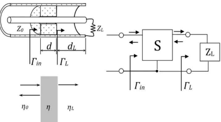
Consider a sample, as shown in Fig. 3, inside a coaxial cable with a termination impedance
connected immediately after the sample (dL=0) or the medium 3 with an intrinsic impedance different
of that of the medium 1 in free-space. In both cases, it is possible to model the system as a slab
represented by its scattering parameters and loaded by impedance ZL or an infinite medium of
intrinsic impedance ηL.
Fig. 3. MUT in transmission line and free space with load.
The reflection coefficient at the input can be obtained from the scattering parameters and the
reflection coefficient at the load from [19] [20]:
Γ
in=
S
11
−
∆
sΓ
L1
−
S
22Γ
L(26)
Where ΔS = S11S22 – S12S21. Considering the sample reciprocity:
Γ
in=
S
11
−
S
11 2−
S
21 2
(
)
Γ
L1
−
S
11
Γ
L(27)
If the load impedance is made equal to the characteristic impedance of the line loaded with the
sample, the reflection coefficient at the input will be that of an infinite sample. This is due to the fact
that, without reflection at the second interface, the wave will only exist in the positive direction from
the input of the sample. Any load or infinite slab with the same impedance as the medium being
measured will present the same reflection coefficient Γ when considered in relation to the input
medium. From these considerations, it follows that if the substitution Γin = ΓL = Γ is done in (27), it is possible to obtain the reflection coefficient at the interface as a function of the slab scattering
parameters:
Γ
1
−
S
11
Γ
(
)
=
S
11
−
S
112
−
S
21 2
(
)
Γ
∴
Γ
2−
S
112
−
S
21 2
+
1
(
)
S
11Γ
+
1
=
0
d$
ΓL$
Γin$
dL$
Z0$ ZL$
η0$ η$ ηL$
S!
ZL!
Γ
=
S
11 2−
S
21 2+
1
±
S
11 2
−
S
21 2+
1
(
)
2−
4
S
11 2
2
S
11
(28)
The sign in (28) must be chosen in a way that |Γ|≤1. Defining:
K! S11 2 −S 21 2 +1 2S 11 (29)
Equation (28) can then be written as:
Γ=K ± K2−1 (30)
Equations (29) and (30) are presented in [6] and [7] as a fundamental part of the NRW algorithm.
The scattering matrix relates the electric fields in the sample, as shown in Fig. 1, in the form:
!
!
E
1 −=
S
11
E
1+
+
S
12
E
3−
E
3
+
=
S
21
E
1+
+
S
22
E
3−
The incident field in the load is E3 +
and the reflected is E3
-. The reflection coefficient at the load, ΓL
is given by:
Γ
L = E3−
E3
+ (31)
Since the system is symmetrical S22 = S11 and the material is isotropic and homogeneous, then S12 =
S21. From (31), E3
-=ΓLE3 +
, the above equation system can be written as:
!
!
E
1 −=
S
11
E
1+
+
S
21
Γ
LE
3+
E
3
+
=
S
21
E
1+
+
S
11
Γ
LE
3+
We can add these two equations and obtain an equivalent system with the same solution. The sum
result is that:
!
!
E
3+
+
E
1−
=
S
11
+
S
21(
)
E
1
+
+
S
21+
S
11(
)
Γ
LE
3+
(32)
Since in the proposed situation, there is not a reflected wave inside the sample and Γin = ΓL = Γ, it
follows:
Γ= E1
−
E1+ (33)
Similarly, the propagation factor is given by:
T = E3
+
E1
+ (34)
From these equations we can evaluate expressions for E3+ e E1-, which are substituted in (32), with ΓL= Γ:
!
!
TE
1 ++
Γ
E
1+
=
S
11
+
S
21(
)
E
1 +
+
S
21
+
S
11(
)
Γ
TE
then:
T = S
11+S21+Γ
1− S
11+S21
(
)
Γ (35)Equation (35) shows the propagation factor as a function of the scattering parameters and the
reflection coefficient at the interface presented in [5] and [6]. The NRW algorithm to determine the
permittivity from the MUT scattering parameters is fulfilled when (2) is considered and then:
ε
r=
1
− Γ
1
+
Γ
⎛
⎝⎜
⎞
⎠⎟
2(36)
And from (4):
ε
r=
j
c
ω
d
ln T
( )
⎛
⎝⎜
⎞
⎠⎟
2
(37)
The equations (36) and (37), isolated or combined, can be used for permittivity determination [21].
The use of (36), as described in [12] will result in a permittivity explicit expression, independent of
the sample size. However this leads to indeterminations when the sample length is a multiple of half
wavelength in low loss materials. The authors conducted an uncertainty analysis as a function of the
permittivity of the measured material and of the sample size. Equation (37) does not show these
problems, but it depends on the sample length, which leads to phase ambiguity problems since T is
complex and its logarithm may have infinite solutions [22].
B. Reflection only methods
If in fig. 3, since dL = 0 and the load is a short-circuit, we have the method known as SCTL
(short-circuit transmission line). This method is also applied to the free-space [4] where the short-(short-circuit is
made through a metal back (metal-back method). Other load types are possible. The model in fig. 3
can be used with any load. The sample scattering parameters, as functions of the propagation factor T
and of the reflection coefficient at the interface Γ, are given in (19) and (25). In a distinct approach
from the deduction of the NRW algorithm, which is intended to write Γ as a function of scattering
parameters only, we now want an expression for the input reflection coefficient Γin, given by (27), as a
function of the factor T and of the coefficient at the interface Γ. When substituting (19) and (25) in (27) (obtained from (26)), then:
Γ
in=
Γ
(
1
−
T
2)
− Γ
L
Γ
2−
T
2(
)
1
− Γ
2T
2− Γ
LΓ
(
1
−
T
2)
(38)C. Double reflection methods – same size samples and different loads.
It is possible to obtain an explicit equation for the permittivity from (38) through the double
same sample with two different loads. These measurements result in the input reflection coefficients
Γ1 e Γ2 from the respective loads ΓL1 e ΓL2. For each one of the loads the propagation factor T can be isolated in (38) with Γgiven by (2):
T2=
ΓL
ε
r −1(
)
+ε
r +1 ⎡⎣⎢ ⎤⎦⎥ Γin
(
ε
r +1)
+ε
r −1 ⎡⎣⎢ ⎤⎦⎥
ΓL
ε
r +1(
)
+ε
r −1 ⎡⎣⎢ ⎤⎦⎥ Γin
(
ε
r −1)
+ε
r +1 ⎡⎣⎢ ⎤⎦⎥
(39)
Thus, if ΓL=ΓL1=-1 (short circuit) in the first measurement and ΓL=ΓL2=1 (open circuit) in other measurement, are applied to equation (39) and compared, the permittivity as a function of two
reflection coefficients Γ1 and Γ2 is:
ε
r=
Γ
1−
1
(
)
Γ
2
−
1
(
)
Γ
1+
1
(
)
Γ
2
+
1
(
)
(40)The normalized input admittance of a transmission line is given by [19]:
y
=
Y
Y
0=
−
Γ −
1
Γ
+
1
(41)Therefore, the permittivity of a sample, when obtained from two measurements, one terminated in a
short-circuit and the other terminated in an open-circuit, is given by:
ε
r = yayc (42)
The permittivity as a product of a short-terminated line admittance (yc) by an open-circuit
terminated line admittance (ya) has already been shown in [14].
D. New double reflection explicit equations
When measuring the reflection coefficient of a short terminated sample and, then, of an impedance
matched terminated sample (ΓL1=-1 e ΓL2=0), it is possible to obtain another explicit equation from
(39):
ε
r=
Γ
2
Γ
1−
3
Γ
2+
Γ
1+
1
Γ
2
Γ
1+
Γ
2+
Γ
1+
1
(43)
Applying the same procedure, but with an open-circuited load in place of the short-circuited one
and, then, of an impedance matched terminated sample (ΓL1=1 e ΓL2=0), the permittivity is now given
by:
ε
r=
Γ
2
Γ
1− Γ
2+
1
− Γ
1Γ
2
Γ
1+
3
Γ
2+
1
− Γ
1(44)
This equation has been derived earlier [15], but its derivation uses a different procedure.
The equations (43) and (44) are particular cases of a general equation. Given any two loads ΓL1 and
ΓL2 (with two measurements Γ1 and Γ2 being done with these two loads), the general explicit equation
ε
r=
Γ
L1
Γ
L2Γ
1− Γ
L1Γ
L2Γ
2− Γ
L1Γ
2Γ
1+
Γ
L2Γ
2Γ
1+
2
Γ
L1Γ
2−
2
Γ
L2Γ
1− Γ
L1+
Γ
L2− Γ
2+
Γ
1Γ
L1
Γ
L2Γ
1− Γ
L1Γ
L2Γ
2− Γ
L1Γ
2Γ
1+
Γ
L2Γ
2Γ
1−
2
Γ
L1Γ
2+
2
Γ
L2Γ
1− Γ
L1+
Γ
L2− Γ
2+
Γ
1(45)
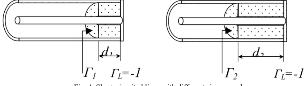
E. Double reflection methods – same loads and different size samples
Using two samples with different lengths, arranged on a short-circuited line, as shown in Figure 4,
it is possible to obtain the permittivity and the permeability. This procedure appears in [11] and [23].
Fig. 4. Short-circuited lines with different sizes samples.
An explicit equation for the permittivity can be obtained considering ΓL=-1 in (39):
T2 =−
Γ
1
(
ε
r +1)
+ε
r −1⎡
⎣⎢ ⎤⎦⎥
Γ
1
(
ε
r −1)
+ε
r +1⎡
⎣⎢ ⎤⎦⎥
(46)
By measuring with sample widths d2 = α d1 the squared propagation factor is given by:
T2 = −
Γ2
(
ε
r +1)
+ε
r −1 ⎡⎣⎢ ⎤⎦⎥
Γ2
(
ε
r −1)
+ε
r +1 ⎡ ⎣⎢ ⎤⎦⎥ ⎛ ⎝ ⎜ ⎜ ⎞ ⎠ ⎟ ⎟ 1 α (47)where αis a scaling fator.
Knowing the relationship between the widths and measuring the reflection coefficients, it is
possible, for certain α values, to obtain explicit expressions for the permittivity considering the
equation:
−
Γ
1(
ε
r+
1
)
+
ε
r−
1
⎡
⎣⎢
⎤
⎦⎥
Γ
1(
ε
r−
1
)
+
ε
r+
1
⎡
⎣⎢
⎤
⎦⎥
⎛
⎝
⎜
⎜
⎞
⎠
⎟
⎟
α=
−
Γ
2(
ε
r+
1
)
+
ε
r−
1
⎡
⎣⎢
⎤
⎦⎥
Γ
2(
ε
r−
1
)
+
ε
r+
1
⎡
⎣⎢
⎤
⎦⎥
(48)
In [11], the widths are set as d2 = 2 d1 (or α = 2). Equation (48) can then be solved explicitly,
obtaining the permittivity:
ε
r =Γ 1−1
(
)
Γ1Γ2−3Γ1+3Γ2−1
(
)
Γ 1+1
(
)
2 Γ 2+1(
)
(49)Employing the same procedure, starting from equation 39 but forcing the samples to end with a
matched load or an absorbing material in free space, another explicit equation for the permittivity can
be obtained:
d
1Γ
L=-1
Γ
1d
2Γ
L=-1
ε
r=
Γ
1−
1
(
)
Γ
1
Γ
2−
2
Γ
1+
Γ
2(
)
Γ
1+
1
(
)
Γ
1
Γ
2+
2
Γ
1− Γ
2(
)
(50)V. ACCURACY
To estimate the uncertainty of the new equations, the Monte Carlo method is applied. The error
sources considered are the finite accuracies of the measured reflection coefficient (within 3% of the
nominal value for amplitude and phase) and of the load impedance (taken to be within 1% of nominal
value). The combined effect of these error sources is computed for a population of 5000 samples in a
rectangular distribution. A low-loss material with ε= 4 – 0,2j and 25 mm width was used.
The standard deviation in permittivity generated by these error sources when applied to equations
(36) (obtained from (28), NRW method), (40) and (43) are shown in Fig. 5 and Fig. 6, for the real and imaginary parts of the permittivity, respectively. When the same errors sources are applied to (49) and
(50), the results are shown in Fig. 7 and Fig. 8, for the real and the imaginary parts of the permittivity, respectively.
Fig. 5. Same size – different loads. Standard deviation of the real part of the permittivity.
Fig. 6. Same size – different loads. Standard deviation of the imaginary part of the permittivity.
to the traditional method of (40). Minimal uncertainty in frequencies 1.5, 4.5 and 7.5 GHz is found for
(43), whereas (40) has an instability. It also can be noted that (43) has, in the entire band, a lower
uncertainty for the imaginary part (when compared to the NRW method). The uncertainty for the real
part of permittivity in quarter-wavelength frequencies (1.5, 4.5 and 7.5 GHz) is slightly higher for
(43) than for the NRW method, but for half-wavelength frequencies the precision of (43) is higher
than the NRW.
Fig. 7. Same load – different sizes. Standard deviation of the real part of the permittivity.
Fig. 8. Same load – different sizes. Standard deviation of the imaginary part of the permittivity.
In Fig. 7 and Fig. 8, it can be observed, that the different-size-samples method, which uses matched loads, shows a lower error along most part of the band.
For both equations the uncertainties get smaller (and closer to one another) as the frequency
increases. This can be due to the larger number of wavelengths inside the material sample width (a
virtual thickening), resulting in larger attenuation and less signal being reflected at the termination.
VI. CONCLUSION
this model the equations for classical NRW algorithm and SCTL method can be derived. Explicit
equations to determine the permittivity were obtained from the new model. In addition to this, two
new equations for the double reflection method were evaluated. One of them uses a short circuit load
and a matched load and the other uses an open-circuit load and a matched load. A new equation is
also obtained for the method with different sizes terminated in the same load, in this case, a matched
one. The uncertainty of the new equations is calculated using the Monte Carlo method and, in both
cases, it is lower than the classical methods. These methods were used for TEM waves in the
free-space and in transmission lines. However, they could be easily extended for waves and samples in
rectangular waveguides.
REFERENCES
[1] S. Kharkovsky and R, Microwave and Millimeter Wave Nondestructive Testing and Evaluation,” IEEE Instrumentation and Measurement Magazine, vol. 10 (2), pp. 26-38, April 2007.
[2] K. Kupfer, Electromagnetic Aquametry – Electromagnetic Wave Interation with Water and Moist Substances, Berlin: Springer-Verlag, 2005, 529p.
[3] A. Von Hippel, editor. Dieletrics Materials and Applications. Cambridge,MA: Technology Press of MIT., 1954, 438p. [4] L. F. Chen, et al., Microwave Electronics Measurement and Materials Characterization. Chichester: John Wiley &
Sons, 2004. 537 p.
[5] D. M. Pozar, Microwave Engineering – Third Edition. New York, NY: John Wiley & Sons. 2005. 700 p.
[6] A. M. Nicolson, and G. F. Ross. “Measurement of the Intrinsic Properties of Materials by Time-Domain Techniques”. IEEE Trans. Instrum. Meas., vol. IM-19, No. 4, pp. 377-382, Nov. 1970.
[7] W. B. Weir. “Automatic Measurement of Complex Dielectric Constant and Permeability at Microwave Frequencies”, Proceedings of the IEEE, vol. 62, No. 1, pp. 33-36, Jan. 1974.
[8] S. Roberts and A. von Hippel. “A New Method for Measuring Dielectric Constant and Loss in the Range of Centimeter Waves”. J. Appl. Phys., vol. 17, pp. 610-616, April 1946.
[9] M. G. Corfield, J. Horzelski and A. H. Price.”Rapid method for determining v.h.f. dielectric parameters for liquids and solutions using standing wave procedures” British Journal of Applied Physics, vol. 12, pp. 680-682. Dec. 1961. [10] S. O. Nelson, L. E. Stetson, and C. E. Schlaphoff. “A General Computer Program for Precise Calculation of Dielectric
Properties From Short-Circuited-Waveguide Measurements”. IEEE Trans. Instrum. Meas., vol. IM-23, No. 4, pp. 455-460, Dec. 1974.
[11] U. C. Hasar, J. J. Barroso, C. Sabah, and Y. Kaya.”Resolving Phase Ambiguity in the Inverse Problem of Reflection-only Measurement Methods”. Progress In Electromagnetics Research , vol. 129, pp. 405-420, June 2012.
[12] S. S. Stuchly and M. Matuszewski. “A Combined Total Reflection-Transmission Method in Application to Dielectric Spectroscopy”. IEEE Trans. Instrum. Meas., vol. IM-27, No.3, pp. 285-288, Sept. 1978.
[13] D. K. Ghodgaonkar, V. V. Varadan, and V. K. Varadan. “Free-Space Measurement of Complex Permittivity and Complex Permeability of Magnetic Materials at Microwave Frequencies”. IEEE Trans. Instrum. Meas., vol. 39, No. 2, pp. 387-394, April 1990.
[14] M. A. Stuchly, and S. S. Stuchly. “Coaxial Line Reflection Methods for Measuring Dielectric Properties of Biological Substances at Radio and Microwave Frequencies – a Review”, IEEE Trans. Instrum. Meas., vol. IM-29, No. 3, pp.176-183, Sept. 1980.
[15] S. L. S. Severo, Aquametria por microondas: desenvolvimento de transdutor em microfita, Programa de pós-graduação em engenharia Elétrica, Dissertação de Mestrado, Universidade Federal do Rio Grande do Sul. Porto Alegre 2003. [16] J. Baker-Jarvis, E. J. Vanzura, and W. A. Kissick.”Improved Techique for Determining Complex Permittivity with the
Transmission/Reflection Method”, IEEE Trans. on Microwave Theory and Techniques, vol. 38, no. 8, pp. 1096-1103, Aug. 1990.
[17] U. C. Hasar, J. J. Barroso, M. Bute, Y. Kaya, M. E. Kocadagistan, and M. Ertugrul. “Attractive method for thickness-independent permittivity measurements of solid dielectric materials”. Sensors and Actuators A: Physical, vol. 206, pp. 107-120, Feb. 2014.
[18] U. C. Hasar and M. T. Yurtcan, "A microwave method based on amplitude-only reflection measurements for permittivity determination of low-loss materials," Measurement , vol. 43, no. 9, pp. 1255-1265, Nov. 2010.
[19] R. J. Weber, Introduction to microwave circuits – Radio frequency and design applications, New York, NY: IEEE Press, 2001,432p.
[20] D. M. Pozar, Microwave Engineering – Third Edition, New York, NY: John Wiley & Sons. 2005. 700 p.
[21] A. Boughriet, C. Legrand and A. Chaponton, “Noniterative Stable Transmission/Reflection Method for Low-Loss Material Complex Permittivity Determination”, IEEE Transactions on Microwave Theory and Techniques, vol. 45, no. 1, pp. 52-57, January 1997