ARCHIVES
Of
FOUNDRY ENGINEERING
Published quarterly as the organ of the Foundry Commission of the Polish Academy of Sciences
ISSN (1897-3310)
Volume 11
Issue 2/2011
95–100
19/2
Application of time-series analysis
for prediction of molding sand properties
in production cycle
M. Perzyk
P a,P
*, S. Maciejak
P aP
, J. Koz
ł
owski
P aP
P
a
P
Institute of Manufacturing Technologies, Warsaw University of Technology, Narbutta 85, 02-524 Warszawa, Polska
* Corresponding author. E-mail address: M.Perzyk@aster.pl
Received 11.04.2011; accepted in revised form 26.04.2011
Abstract
Time-series analysis is characterized, as a data mining tool which facilitates understanding nature of manufacturing processes and permits prediction of future values of the process parameters or production results on the basis of the past data, recorded in regular intervals. The main methods and problems of the time-series analysis are presented. The authors’ research results, based on green molding sand proper-ties data collected in a foundry with Disamatic molding line, are presented. The work was aimed at finding optimal settings and models of the time-series analysis for that data as well as detection of possible periodicities appearing in the sand properties. It is concluded that although the time-series analysis requires individual approach to each particular problem, some general recommendations can be also formulated. It can be a useful tool for analysis and predictions of outcomes of foundry processes.
Keywords:Tdata mining,time-series analysis, foundry technology, molding sand propertiesT.
1. Introduction
Time-series analysis deals with series of data recorded in a chronological order, usually in regular time intervals or in another sequences. The main goal of the analysis, being one of the data mining techniques, is to facilitate finding some important charac-teristics of processes as well as prediction of the future results. The time-series prediction can be considered as a particular case of a regression task, where the input and output variables are the same quantity but measured at different time moments.
It has been recognized that an application of these methods in manufacturing industry can bring various benefits (see e.g. [1-4]). Detection of periodicity in products’ or materials’ properties in a foundry can facilitate identification of the irregularities in the manufacturing processes. Prediction of the process parameters or
the product properties in a near future can help to prevent un-wanted tendencies or suggest required changes in the process control.
by taking the above mentioned input – output sets, shifted by one point in the series. The composition of the records for regression model should be preceded by subtraction of the general trend (usually linear), the periodical component and, possibly, the variability amplitude trend. The idea of this methodology is to use a regression model for modeling finer changes than those which can be easily described by simple trends and periodicity.
For the calculation of the trend of variability amplitude, the authors own methodology was applied, presented in [6].
Calculation of the periodical component should be preceded by the significance analysis of the periodicity appearing in the time-series. The appropriate analysis is based on the autocorrela-tion coefficient and is described in [6]. After determinaautocorrela-tion of the periodicity, a centered periodical component is calculated and subtracted from the time-series (without trends); details can be found in [5].
Thus obtained residual data can be used for regression model-ing. However, a question arises if these data contain important information or they are simply a random noise. In the second case the modeling would be certainly unsuccessful. To answer this question some statistical tests can be applied. One of them is the non-parametric runs-test that verifies a randomness hypothesis for a binary-valued data sequence; in case of time-series, the signs of the residual values of the time-series. Another test as-sumes, that if the residual component is of random nature then it is characterized by a low autocorrelation coefficient. In particular, the autocorrelation of the first order is tested (i.e. for time lag equal to 1), using the Durbin-Watson test. The description of the both tests can be found in [7]).
The purpose of the present research was to find optimal set-tings and models of the time-series analysis for the real foundry data including recorded properties of green molding send as well as detection of possible periodicities appearing in the sand prop-erties.
2. Research plan and methodology
2.1. Data sets
All data used in the present work have been obtained from a Polish grey cast iron foundry, equipped with two Disamatic molding lines (2110 Mk3 and 2110 Mk5 with a sand cooling system. The original source data included 624 records collected during three summer months, in 39 working days (16 records per day in 1 hour intervals). The following green sand properties were measured and recorded: moisture content of used and fresh sands, compression strength, permeability, compactibility, and temperatures of used and fresh sands.
Two types of series data were used. The first one, further re-ferred to as ‘hourly based’, assumes 1 hour time intervals and utilizes all the source data, placed consecutively in order of their recording.
The second type of series data, further referred to as ‘daily based’, was aimed at analysis of the sand properties variability on a daily basis. For each sand property the following three quanti-ties were calculated from the values recorded each day: the first measurement of a given day, the average of the 3 first measure-ments of the day and the average value of the whole day. Because some periodicity can be expected, related to week periods, it was
essential that only repeatable sequences of week days were in-cluded in the sets used for the analysis. However, on some work-ing days the production was not run and it was necessary to re-duce the data, so that only 6 week periods, each containing 4 first days (from Monday to Thursday), could be selected.
Summarizing, the total number of serial data sets prepared for the time-series analysis for the hourly based type data was 7 (each containing 624 elements) and total number of serial data sets for the daily based type data was 21 (each containing 24 elements).
2.2. Details of time-series analysis
There are several decisions which should be made before time-series analysis can be performed. First, the number of points used as inputs and the distance of prediction (from the last input) should be determined. In the present work two numbers of inputs were applied: 5 and 9, and 3 distances of prediction equal 1, 2 and 3 were assumed.
The periodicity appearing in the data can be statistically sig-nificant or non sigsig-nificant. In the latter case a question arises if the periodical component should be subtracted or not. In the present work the accuracy of prediction was tested for such cases and the appropriate conclusion was drawn.
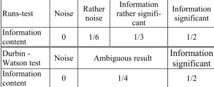
The information content included in the residual data, i.e. af-ter subtraction of trends and periodical component, can be evalu-ated on the basis of the two statistical tests discussed earlier. However, they can give divergent results and also each of them can provide uncertain information. For the purpose of the present work the variable called ‘information content’, valued between 0 and 1, was proposed. It is calculated as a sum of the values ob-tained from the two tests, given in Table 1.
Table 1. Residual data information contents dependent on the statistical tests results
Runs-test Noise Rather noise
Information rather
signifi-cant
Information significant
Information
content 0 1/6 1/3 1/2
Durbin
-Watson test Noise Ambiguous result
Information
significant
Information
content 0 1/4 1/2
The basic model used for residual data was simple linear mul-tivariate regression. However, for the 10 cases with largest pre-diction errors, also a regression tree model, based on the C&RT algorithm [8], was utilized. The regression trees are non-parametric, non-linear models which are particularly suitable for small data sets with unknown characteristics. Because of the small number of records for the daily based data, the regression tree algorithm was set to keep only 2 records in a leave. The prediction results were compared with those obtained from the linear model.
3. Results
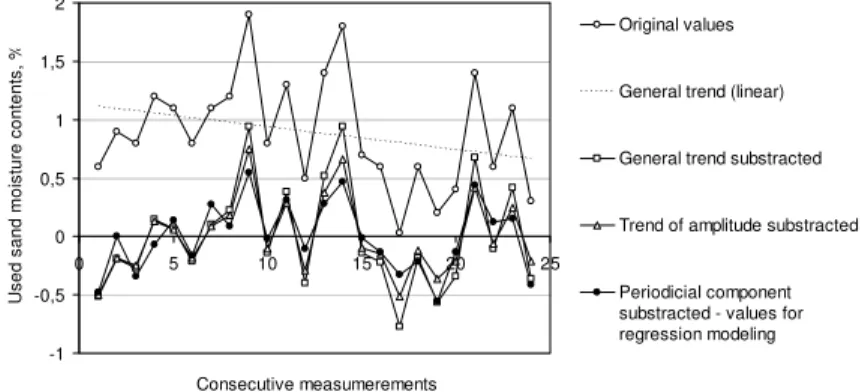
In Fig. 1 exemplary results of initial steps in time-series analysis are shown, illustrating the magnitude of particular com-ponents described in section 1.
For majority of the hourly based type data sets the periodicity appeared to be statistically significant and equal to 2, except for compression strength, where it was insignificant. The probable interpretation is that 2 hours period is strongly related to the molding sand processing cycle time. By contrast, for the majority of daily based type data sets, the periodicity was insignificant, except for the used sand temperature, where it was significant and equal to 4. This result may indicate that the molding sand proc-essing was stable and resistant to the temperature perturbations,
possibly related to the position of a day in a week (e.g. after weekends).
For all hourly based data sets the information content in re-sidual data was equal 1. It means that both statistical tests explic-itly indicated that the residual data may include important infor-mation and therefore it is advisable to apply a regression model for finding desired predictions. By contrast, for most of the daily based data sets the information content in residual data was below 0,5, (in almost half of the cases it was equal to zero). Taking into account that the residual data are important fraction of the whole variability in those sets (an example is shown in Fig. 1), these results indicate that the time-series analysis can give prediction results with relatively large errors.
-1 -0,5 0 0,5 1 1,5 2
0 5 10 15 20 25
Consecutive measumerements U s e d s a nd m o is ture c o nte n ts , % Original values
General trend (linear)
General trend substracted
Trend of amplitude substracted
Periodicial component substracted - values for regression modeling
Fig. 1. Example of the consecutive steps of the time-series analysis: the daily-type data for used sand moisture content
An evaluation of the magnitude of relative error of prediction can be made by its comparison to relative absolute deviations appearing in the data. For all hourly based data the average rela-tive error of predictions was about 2,7% and the average relarela-tive absolute deviation for that data was about 12,1%. This result means that the time-series analysis can be a useful prediction tool for that type of data. By contrast, for the daily based data the average relative error of predictions was about 34% and the aver-age relative absolute deviation for that data was about 13%. This result confirms the low usefulness of the time-series analysis for prediction of future values when the noise component is relatively large. 0 1 2 3 4 5 6
5-1 5-2 5-3 9-1 9-2 9-3 Number of inputs - distance of predicted
output A v e rag e r at io of pr e di c tion er ror s f or no n-s ign ifi c an t per iodi c ity ignor ed /s ubtr a c ted
Fig. 2. Effect of subtraction of non significant periodicity on prediction errors for all data sets, for various numbers of inputs
and prediction distances
The subtraction of periodical component can be made in spite of its statistical significance, just to reduce the variability in the data used for the regression model. The predictions were made for all data sets with non-significant periodicities in two versions: with the periodicity ignored and subtracted.
In Fig. 2 the ratio of prediction errors for all data sets with non- significant periodicity for the above two versions are shown. It can be seen that the prediction errors are substantially reduced by subtraction of the insignificant periodicity before regression modeling. 0 1 2 3 4 5 6 7 8 9 10
1 point forward 2 points forward 3 points forward Distance of predicted output
R at io of pr edic tio n er ror s f or num ber s o f input s 9/ 5
Fig. 3. Effect of number of inputs on prediction errors for daily based data (open circles) and hourly based data (solid black
It was found that increasing the number of input points not only makes the regression model more complex, but can lead to remarkable larger prediction errors. This is shown in Fig. 3, where the ratio of prediction errors for numbers of inputs equal to 9 to that equal to 5 is plotted. for both types of data sets.
In Fig. 4 the relative prediction errors are plotted vs average relative errors for training data. It can be seen that increasing the number of inputs significantly decreases only the training error. It can be also seen that the cases which are more difficult to learn (train) are not necessarily more difficult to predict (the correlation between the two errors is very low).
R2
= 0,045 R2
= 0,001
0% 10% 20% 30% 40% 50% 60%
0% 5% 10% 15% 20%
Relative training error
R
e
la
tiv
e
pr
ed
ic
tion
er
ro
r
Number of inputs = 5
Number of inputs = 9
Fig. 4. Relative prediction errors vs average relative errors for training data, for all data sets of both types
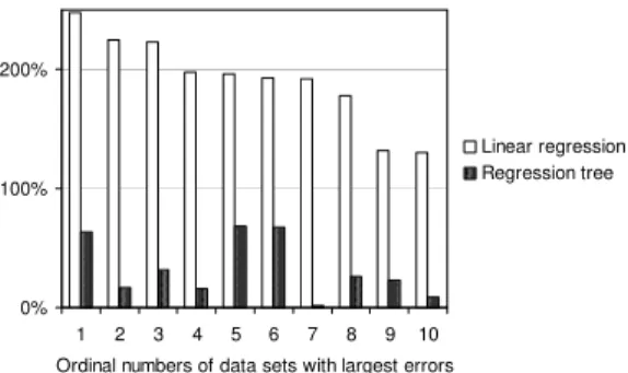
For the data sets with the largest prediction errors (of daily type) a more advanced regression model was tried out. In Fig. 5 the regression modeling relative errors obtained from the linear and tree-type models are compared; note that these values are no prediction errors but are merely related to the residual data.
0% 100% 200%
1 2 3 4 5 6 7 8 9 10 Ordinal numbers of data sets with largest errors
Linear regression Regression tree
Fig. 5. Relative regression modeling errors for the 10 cases with the largest prediction errors
A radical rise of the modeling accuracy can be observed due to application of the tree type regression model instead of the simple linear one.
4. Summary and conclusions
The presented research has demonstrated some important fea-tures of time-series analysis from the standpoint of its application to real industrial manufacturing processes. It was shown that application of that kind of data mining tool can provide a signifi-cant insight in the process and predict its future results, i.e. the
product properties or process parameters. Although the research was based on data obtained in specific conditions, some observa-tions can be treated as applicable to a wider range of processes.
In particular, it can be recommended, that the periodical com-ponent of the series data should be always subtracted prior to final regression modeling, even when the periodicity is statistically non-significant. This can facilitate the regression modeling and can lead to lower prediction errors.
Another finding is that the simple linear regression model may be unsatisfactory for modeling more complex relationships included in the residual data. The regression trees turned out to be a promising type of model, especially when the number of train-ing records is small. However, for larger sets, also some other advanced models should be considered, e.g. artificial neural net-works [5].
In spite of above general findings, it should be emphasized, that the time-series analysis always requires individual approach to the problem. In particular it applies to such problems like set-ting number of input points, choosing type of the general trend type (linear or curved), use the final regression model when the information content in residual data is relatively low, etc.
Acknowledgment
This work was partly supported by Ministry of Science and Higher Education of Poland, project No. N R07 0015 04.
References
[1]S. Bisgaard, M. Kulahci, Quality quandaries: Using a time-series model for process adjustment and control, Quality En-gineering, vol. 20 (2008) 134–141.
[2]Z.C. Lin, D.Y. Chang, A band-type network model for the time-series problem used for IC leadframe dam-bar shearing process, International Journal of Advanced Manufacturing Technology, vol. 40, No. 11-12 (2009).
[3]S.G. Kapoor, R.W. Terry, Time-series analysis of tensile strength in a die casting process, Time-series Analysis: The-ory and Practice 4, Proc. 8th International Time-series Meet-ing and 3rd American Conference, 1983, 221-228.
[4]F.R. Camisani-Calzolari, I.K. Craig, P.C. Pistoriust, Quality prediction in continuous casting of stainless steel slabs, Jour-nal of The South African Institute of Mining and Metallurgy, vol. 103, No. 10 (2003), 651-665.
[5]T. Masters, Sieci neuronowe w praktyce. WNT Warszawa 1996.
[6]M. Perzyk, K. Krawiec, J. Kozłowski, Application of time-series analysis in foundry production, Archives of Foundry Engineering, vol. 9, No.3 (2009), 109-114.
[7]B. Borkowski, H. Dudek, W. Szczęsny. Ekonometria. Wybra-ne zagadnienia. PWN, 2004