Brazilian Journal of Physics, vol. 36, no. 3B, September, 2006 963
Dynamical Phase Transition in Vibrational Surface Modes
H. L. Calvo and H. M. Pastawski
Facultad de Matem´atica, Astronom´ıa y F´ısica, Universidad Nacional de C´ordoba, Ciudad Universitaria, 5000 C´ordoba, Argentina
Received on 8 December, 2005
We consider the dynamical properties of a simple model of vibrational surface modes. We obtain the exact spectrum of surface excitations and discuss their dynamical features. In addition to the usually discussed local-ized and oscillatory regimes we also find a second phase transition where the surface mode frequency becomes purely imaginary and describes an overdamped regime. Noticeably, this transition has an exact correspondence to the oscillatory - overdamped transition of the standard oscillator with a frictional force proportional to veloc-ity.
Keywords: Dynamical phase transition; Vibrational localized states; Origin of frictional forces
I. INTRODUCTION
In a classical oscillator, dissipation is described considering an equation of motion with a friction term proportional to the velocity [1]. Ignoring microscopic details, all environmental effects are summarized phenomenologically in the coefficient η0of this term. We propose here a simple and time-reversal invariant model whose analytical solution yield dissipation in the thermodynamic limit. We consider a variation of the Ru-bin model [2, 3] shown in Fig.1: a ”surface” oscillator (repre-sented as a pendulum) with natural frequencyω0and massm0 coupled to an ordered and semi-infinite chain of ”bulk” oscil-lators whose masses arem. As occurs with a “Brownian bath” [4], Ohmic dissipation will requireα=m/m0≪1.
FIG. 1: Scheme of the model: a simple pendulum (surface oscillator) is coupled to the bulk masses.
The equations of motion are,
· d2 dt2+ω
2 0+αω2x
¸
u0(t)−αω2xu1(t) =0, ·
d2 dt2−2ω
2
x
¸
un(t)−ω2x[un−1(t) +un+1(t)] =0, (1)
whereωx=
p
K/mis the exchange frequency between neigh-bor oscillators and un(t)denotes the nth oscillator
displace-ment from equilibrium. Assuming that the number of bulk os-cillators is finite, the time-reversal invariance present in these equations is obvious. We will show below how irreversibility appears in the thermodynamic limit where the number bulk oscillators become infinite.
II. FREQUENCY DOMAIN
The equations of motion described above can be solved by Fourier transforming the displacement:
un(t) =
1 2π
Z ∞
−∞dωe
−iωtu
n(ω), (2)
and replacing it in Eq.(1):
¡
ω2I−M¢u(ω) =0. (3)
This equation is solved by the eigenfrequencies ωk and
eigenvectorsu(ωk)whose site components are expressed, in
bracket notation, in terms of the site versorshn|as
un(ωk) =hn|ϕki, (4)
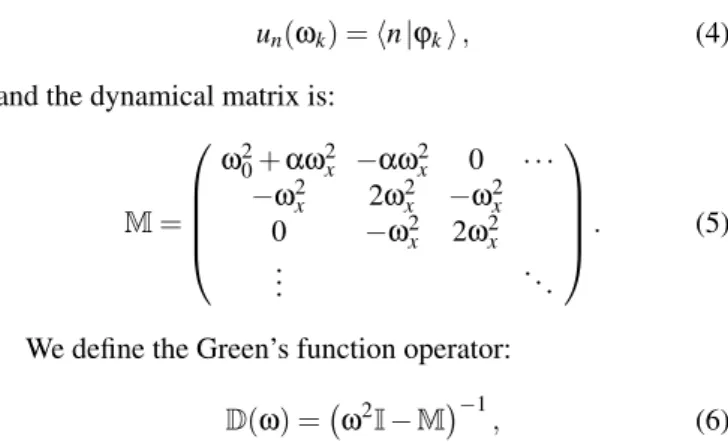
and the dynamical matrix is:
M=
ω2
0+αω2x −αω2x 0 ···
−ω2
x 2ω2x −ω2x
0 −ω2
x 2ω2x
..
. . ..
. (5)
We define the Green’s function operator:
D(ω) =¡ω2I−M¢−1, (6)
whose matrix elements diverge when ω coincides with an eigenfrequencyωk.
Consider an initial condition with all masses at equilibrium and an impulsive forcemju˙j(0)δ(t)applied to the jth mass,
impossing an initial velocity to it. In this case, the Green’s function provides the time evolution of theith mass displace-ment:
ui(t) =Di j(t)u˙j(0) =
1 2π
Z ∞
−∞dω
e−iωtDi j(ω)u˙j(0), (7)
representing a position-velocity Green’s function Di j(ω)≡
D(ui,u˙j;ω), which is related to the position-position Green’s
function:
964 H. L. Calvo and H. M. Pastawski
This gives the displacement of theith mass when an initial displacementuj(0)is imposed by the force:
Fj(t) =mj
uj(0)
τ [δ(t+ 1
2τ)−δ(t− 1
2τ)] (9)
at the jth mass, whereτ≪1/ωx.
In this work, we focus on the surface oscillator through D00(t). IfUis the matrix that performs the change of basis from sites to diagonal form inM, one has:
Uik=hi|ϕki, (10)
that is, thekth eigenmode projection overith site. In this case one can write,
D00(ω) =
∑
k|h0|ϕki|2
ω2−ω2
k
. (11)
By performing the analytical continuationω→ω+iδfor D00(ω)and taking its imaginary component, one obtains the spectral density associated to the surface site. In the case whereα→0 bulk modes and surface modes have no projec-tion and oscillaprojec-tions survive undamped.
D00(ω)can be obtained through an infinite order perturba-tion theory [5] that accounts for the surface mode correcperturba-tions due to the presence of the neighbor oscillators. Let us begin with the surface oscillator and a single bulk mass. If the two masses are uncoupled (ωx=0) the surface frequency is
sim-plyω0but ifωx6=0, Eq.(6) yields
D00(ω) =
1
ω2−ω2
0−αω2x−α
ω4
x
ω2−ω2
x
. (12)
Here, ω0 is affected by the static correctionαω2x and the
dynamic correctionαΠ(ω)due to presence of the other oscil-lator.
By taking the limit of the oscillators number to infinite, the dynamic correction becomes
Π(ω) = ω
4
x
ω2−2ω2
x−Π(ω)
. (13)
Because of the presence of an infinite number of oscillators at the right, a correction on thenth oscillator is just the same as that in the(n+1)th oscillator. The solution of Eq.(13) is complex and its imaginary part gives the decay rate of a sur-face excitation with frequencyω. Therefore, in the thermody-namic limit, the temporal recurrences [6] (Mesoscopic Echoes [7]) disappear.
III. SURFACE MODE FREQUENCY
In the case of a surface oscillator with natural frequencyω0, coupled to an infinite number of bulk oscillators, the Green’s function is:
D00(ω) =
1 ω2−ω2
0−αω2x−αΠ(ω)
. (14)
Hence, in the region of continuous modes (|ω| ≤2ωx) one
has
D00(ω) = 1 1−α2
1 ω2−ω¯2
0+iη(ω)ω
, (15)
where ¯ω0=ω0/ p
1−α/2 is a first approximation to the res-onance frequency and
η(ω) = αωx
1−α2 s 1− µ ω 2ωx ¶2 (16)
describes the dissipation process. Comparing Eq.(15) with a standard damped oscillator (frictional force proportional to velocity), it is easy to see that in the broadband limit (α→0, ωx→∞andαωx=const.) they have the same behavior taking
η0≡αωxas friction coefficient.
For a dynamic description of the surface oscillator, we look for the pole structure ofD00(ω), equivalent to findωsuch that:
ω2−ω¯2
0+iη(ω)ω=0. (17) If we denote the surface mode frequency as ˜ωR=ωR+iγR
andpas
p= ω0−ωx
ωx
√
1−α, (18)
then one has
˜ ωR=
− r ω2 0+δ
h ω2
−+
q ω4
+−4ω2xω20 i
p<−1 r
ω2 0+δ
h ω2
−−i
q 4ω2
xω20−ω4+ i
|p| ≤1 r
ω2 0+δ
h ω2
−−
q ω4
+−4ω2xω20 i
p>1 whereω2
±=ω20±αω2xandδ=α/2(1−α). The dependence
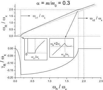
of the pole withω0can be seen in Fig.2.
Here, we show the real and imaginary parts of the pole sep-arately and we find three well-defined regimes that emphasize the onset of quite different dynamical properties.
IV. DYNAMICAL PHASES
Localized - extended transition. This transition occurs whenω0lays close to the upper band edge. There, the real part of the pole makes an excursion into the band gap conserving an imaginary component which is lost at the cusp zoomed in the inset. This is analogous to the virtual states described by Hogreve [8] for electronic states which are missed under other approximations [9, 10]. They become real normalized states which are exponentially localized [11] when the pole touches back the band edge.
It can be seen in Fig.2 that for large values of surface natural frequency(ω0≫2ωx)we only have real component in ˜ωR
Brazilian Journal of Physics, vol. 36, no. 3B, September, 2006 965
0.0 0.5 1.0 1.5 2.0 2.5 -0.20
-0.15 -0.10 -0.05 0.00
R
=2
x
R
/
x
0 /
x
0.0 0.5 1.0 1.5 2.0
c2
/
x c1
/
x
0
= m/m
0 = 0.3
c2
/
x
c1
/
x
R
/
x
FIG. 2: Surface Green’s function pole. Above: real part (resonance). Below: imaginary part (damping). The caseωR=ω0is shown in
dotted line. Insets: overdamped - oscillatory transition (left). Local-ized - extended transition (right).
oscillators increase their distance to the surface. The lack of an imaginary part implies that the displacement amplitude, in-dependently of bulk oscillators, survives indefinitely. In other words, there is no energy propagation towards bulk oscilla-tors.
Asω0decreases, below a critical frequencyωc2=ωx(1+
√
1−α), ˜ωRbecomes complex. Its real part is the resonance
frequency whereas its imaginary part describes the dissipa-tion. This is the extended oscillatory regime where surface oscillations have anωRfrequency and the amplitude of
dis-placement decays with a lifetime proportional to 1/γR.
Oscillatory - overdamped transition. Forω0≪ωx the
system is in the regime where η(ω)≃αωx/(1−α/2) and
hence Eq.(17) yields Ohmic dissipation in which the surface kinetic energy decays into bulk modes without return. This describes a frictional force proportional to the velocity. Asω0 goes below the critical frequencyωc1=ωx(1−
√
1−α), the pole of the Green’s function ˜ωR becomes purely imaginary.
This is the overdamped regime where no oscillations occur. Notice thatγR decreases at both sides of the transition, this
means that a further decrease ofω0or increase in the frictionη also implies adecreasein the relaxation rate. All this counter intuitive effect arises from the exact solution of the simple mechanical model.
Considering Eq.(7), we can complete our previous analysis obtaining the time evolution of surface displacement by per-forming a numerical Fourier transform of the analytical ex-pression forD00(ω). These results coincide with the numer-ical integration of the equation of motion in the Hamilton-Jacobi representation which is performed with anad hoc ver-sion of the Trotter-Suzuki method [12]. Setting the ratioα be-tween masses and Fourier transforming for severalω0values
in the previously mentioned regimes, we obtain the displace-ment pattern shown in Fig.3.
0.0 0.4 0.8 1.2 1.6 2.0 0
2 4 6 8 10
L
o
c
a
l
i
z
e
d
O
v
e
r
d
a
m
p
e
d
Oscillatory Extended
c2
/
x c1
/
x
= m/m
0
= 0.2
0
/
x
T
i
m
e
FIG. 3: Evolution of the surface displacement. White spaces denote
u0(t)>0 whereas gray spaces denoteu0(t)<0.
Here, the time evolution of the surface displacement de-pends on the initial condition. It is easy to see in this picture how the period of the oscillation (reflected from the edges of the gray fringes) diverges near the critical frequencyωc1 so that for smallerω0 valuesu0(t) is always positive. On the other hand, the period shows a cusp atωc2 where it start to increase again. This is consistent with the decrease ofωRas
ω0crossesωc2(see inset in Fig.2).
V. CONCLUSIONS
Dynamical features in dissipation processes have been de-scribed by a simple classical model that contains the essen-tial properties of a surface oscillator interacting with bulk vi-brational modes. We arrive to results equivalent to the phe-nomenological description of dissipation where these effects are summarized in a single term proportional to the oscillator velocity. A complete analytical solution of the dynamics al-lowed us to identify a variety of dynamical phases available for the vibrational excitations: localized, extended oscillatory and overdamped. Two numerical methods (FFT and a Trotter-Suzuki algorithm) have been employed to obtain the dynamics with equivalent results.
966 H. L. Calvo and H. M. Pastawski
[1] R. Feynman,The Feynman Lectures on physics, vol. I, Ch. 23-25, Addison-Wesley, 1970.
[2] T. Dittrich, P. H¨anggi, G.-L. Ingold, B. Kramer, G. Sch ¨on, W. Zwerger,Quantum transport and dissipation, 217, Wiley-VCH, 1998.
[3] R. J. Rubin, Phys. Rev.1313, 964 (1963).
[4] P. H¨anggi and G.-L. Ingold, Chaos15, 026105 (2005). [5] H. M. Pastawski and E. Medina, Rev. Mex. F´ısica 47s1, 1
(2001), cond-mat/0103219.
[6] P. Blaise, P. Durand, and O. Henri-Rousseau, Phys. A209, 51 (1994).
[7] H.M. Pastawski, P. R. Levstein, and G. Usaj, Phys. Rev. Lett.
75, 4310 (1995).
[8] H. Hogreve, Phys. Lett. A201, 111 (1995).
[9] E. N. Economou, Green’s functions in quantum physics, Springer series in solid state physics 7, 1979.
[10] M.C. Desjonqu`eres and D. Spanjaard, Concepts in Surface Physics 2ε, 114, Springer, 1996.
[11] P. L. Taylor,A quantum approach to the Solid State, Prentice-Hall, 290, 1967.