http://dx.doi.org/10.1590/0104-530X2297-16
Resumo: Este trabalho trata do problema de roteamento e programação de navios que transportam óleo cru das plataformas offshore (localizadas no oceano) até os terminais costeiros, motivado por um estudo de caso feito em uma empresa brasileira que realiza essa operação. Com base nesse estudo, propõe-se um modelo de programação inteira mista que é uma extensão do problema clássico de coleta e entrega com janelas de tempo. Esse problema pertence à classe NP-difícil, sendo sua resolução bastante desaiadora na prática. Ao problema da literatura foram agregadas outras restrições práticas relacionadas ao caso em estudo, o que torna a formulação ainda mais desaiadora para resolução direta por meio de softwares de otimização. Em vista disso, dois métodos de solução exatos do tipo branch-and-cut são propostos neste trabalho, os quais usam desigualdades válidas especíicas para o problema em estudo. Os resultados de experimentos computacionais realizados com instâncias reais fornecidas pela empresa mostram que os métodos branch-and-cut propostos resolveram uma quantidade maior de instâncias em comparação com a resolução direta do modelo por meio de software de otimização.
Palavras-chave: Problema de coleta e entrega; Roteamento e programação de navios; Indústria petrolífera; Método branch-and-cut.
Abstract: This paper addresses the routing and scheduling problem of vessels that collect crude oil from offshore platforms (located in the ocean) and transport it to terminals on the coast. This problem is motivated by a case study carried out in an oil company that operates in Brazil. Based on this study, we propose a mixed integer programming model that extends the classical pickup and delivery problem with time windows. This problem belongs to the NP-hard class and its solution is very challenging in practice. To model speciic features of the addressed case, we include new constraints in the classical formulation, which makes it even more challenging for general purpose optimization solvers. To overcome this, we propose two branch-and-cut methods that use valid inequalities especially developed for the oil company case. Computational results performed with a real data set provided by the company show that the proposed branch-and-cut methods are effective and able to solve more instances than a state of the art general purpose optimization solver.
Keywords: Pickup and delivery problem; Ship routing and scheduling; Oil industry; Branch-and-cut method.
The pickup and delivery problem with time
windows in the oil industry: model and
branch-and-cut methods
O problema de coleta e entrega com janelas de tempo na indústria petrolífera: modelos e métodos branch-and-cut
Maria Gabriela S. Furtado1 Pedro Munari1 Reinaldo Morabito1
1 Departamento de Engenharia de Produção, Universidade Federal de São Carlos – UFSCar, Rod. Washington Luís, Km 235, SP-310, CEP 13565-905, São Carlos, SP, Brazil, e-mail: gabisfurtado@gmail.com; munari@dep.ufscar.br; morabito@ufscar.br
Received May 18, 2015 - Accepted Dec. 03, 2015
Financial support: FAPESP – São Paulo Research Foundation (projects 2014/22542-2 and 2014/00939-8), CAPES, Petrobras and the Agência Nacional de Petróleo (ANP).
1 Introduction
Maritime transportation has grown considerably in recent years and the maritime industry is receiving more investment and greater attention from academics (Christiansen et al., 2004). In particular, the oil industry was one of the maritime areas that has been the focus of attention in recent years. In Brazil, the oil production capacity is almost 2.78 million barrels per day. The crude oil exports reach a total
of 3.54 million tons (Brasil, 2011) and the largest reserves are in continental platforms in deep water.
coast. It must be transported within deadlines deined
by time windows at the platforms and terminals. In this paper, we propose a mixed integer programming model to represent the problem of the oil company case. The proposed model is an extension of the classical pickup and delivery problem with time windows (Desaulniers et al., 2002; Ropke & Cordeau, 2009). This extension differs from other literature problems because of
speciic requirements related to the routing and
scheduling problem of oil tankers and the policies
of the company. Due to the dificulty in solving
the resulting model directly by general-purpose optimization software, two branch-and-cut methods were proposed, using specialized valid inequalities that improve the lower bounds provided by the linear relaxation of the model and that ensure the satisfaction of additional requirements concerning the vessels, platforms and terminals. As the total number of valid inequalities is exponential in relation to the number of pickup and delivery requests, it is impractical to generate them a priori. Hence, separation procedures are used in the branch-and-cut methods to analyze when a valid inequality is violated and then add the violated ones in an ad-hoc way.
Therefore, the main contributions of this paper are a mathematical programming model able to represent the company’s problem and solution methods to solve the model more effectively when compared to its solution directly by general-purpose optimization software.
The remainder of this paper is organized as follows. In Section 2, we present a brief literature review regarding the pickup and delivery problem in the oil industry and related branch-and-cut methods. In Section 3, we describe the features of the problem concerning the oil company case and propose a mixed integer programming model. The proposed branch-and-cut methods are described in Section 4, followed by the computational tests in Section 5. Finally, we present the conclusions and future research in Section 6.
2 Literature review
In the pickup and delivery problem, customers are represented by nodes of a network and partitioned as either pickup or delivery nodes. Each node i has a demand qi that must be collected and then delivered to node n+i, with qn+i=-qi (corresponding delivery demand). Hence, the number of pickups and deliveries must be the same. Every pickup node must be visited before the corresponding delivery node (precedence constraints) and both nodes must be in the same route (pairing constraints). Further
details regarding pickup and delivery problems and its applications can be found, e.g. in Berbeglia et al. (2007), Ropke et al. (2007), Nowak et al. (2008), Ropke & Cordeau (2009) and Hennig et al. (2012).
For the pickup and delivery problem with time windows (PDPTW), time window requirements are imposed on the nodes. Dumas et al. (1991) proposed an exact algorithm for the PDPTW, based on column generation, with the shortest path constraints in the subproblem. Lu & Dessouky (2004) proposed a new type of formulation and a branch-and-cut algorithm that uses four classes of valid inequalities. Baldacci et al. (2011) presented an exact algorithm, based on the set partitioning formulation and route relaxation strategy, known as ng-routes. Interesting literature reviews have been presented by Savelsbergh & Sol (1995), Desaulniers et al. (2002), Berbeglia et al. (2007), Cordeau et al. (2008), Parragh et al. (2008a, b).
Ropke et al. (2007) proposed two models for
the PDPTW with 2-index variables. The leet is
unlimited and homogeneous, and it must respect capacity and time window constraints. The objective is to minimize the travel costs. In the proposed models, the number of constraints is exponential with respect to the number of requests, so it is not practical to enumerate them. Therefore, the models were solved by a branch-and-cut algorithm in which
some families of valid inequalities were speciically
proposed for the PDPTW. Ropke & Cordeau (2009) proposed a branch-cut-and-price method for the pickup and delivery problem with time windows. The method uses the valid inequalities presented in Cordeau (2006), Ruland & Rodin (1997) and Ropke et al. (2007), and the computational results showed that the method solved several large-scale instances in a reasonable amount of time. It is worth mentioning that the classical model presented by Ropke & Cordeau (2009) for the PDPTW is used as a basis for the model we propose for the oil company case, to which we incorporate new constraints and a different objective function.
There are many studies in the literature related to vehicle routing and scheduling problems, regarding mathematical models and solution methods. However, the literature is not extensive for studies
speciically involving the routing and scheduling
of vessels. According to Christiansen et al. (2007), this is due to several factors, such as lower visibility and structuring maritime transportation, higher
uncertainty in decision-making, the dificulty of
introducing new ideas into the industry as it is older than the other transportation, among other factors.
One of the irst papers to address the scheduling
the United States Navy for fuel transportation. They proposed a linear programming model in which the objective was to minimize the number of used vessels. They also developed an exact solution method for the problem. In Christiansen (1999), the routing and scheduling problem of vessels with time windows was studied in a company that
transports ammonia. The goal was to ind routes
with minimal transport costs that satisfy minimum and maximum inventory levels. Sherali et al. (1999) studied the scheduling problem of vessels
which transport crude oil and reined products from
Kuwait to Japan and countries in North America
and Europe. The leet was heterogeneous, the
vessels were able to transport different products and time windows were imposed for pickup and delivery nodes. They proposed a heuristic to solve the problem with a rolling horizon time.
Christiansen et al. (2004) reviewed problems related to vessel routing and scheduling, focusing on literature from the 1990s. The paper addresses strategic, tactical and operational decision problems together with a few applications. Rocha et al. (2009) proposed a mathematical model for the oil allocation problem at Petrobras, which involves
decisions related to leet assignment, transporting
different types of oils and the terminal assignment. The objective was to minimize the total costs. This problem differs from the study case problem addressed in this paper, because it involves decisions in a higher hierarchical level and hence their solutions can be used as input data for our problem.
Hoff et al. (2010) presented a literature review that describes the industrial aspects, routing
characteristics, problem classiication and some
strategies presented in the literature to solve the routing and scheduling problem of vessels. Another literature review in maritime transportation is presented in Andersson et al. (2010) that emphasized the decisions and process related to inventory levels, and the combination of these actives in operational research. Formulations and exact methods for the routing and scheduling problem of vessels have also been presented by Hwang et al. (2008), Brønmo et al. (2010), Stålhane et al. (2012), Hennig et al. (2012) and Fagerholt & Ronen (2013).
3 The pickup and delivery problem
in the oil industry
This section describes the routing and scheduling problem of vessels in the oil industry and its main differences regarding classical problems presented in the literature. The focus of this study is crude oil transportation from platforms to terminals. The routing and scheduling problem of vessels
can be found in a context in which the origins
and destinations are ixed. Hence, in a previous
plan, the company decided the quantity of crude oil that must be transported from each platform to each terminal. Therefore, the problem addresses the decision of which vessel should pickup and deliver the crude oil and when this must happen.
3.1 Problem description
Each vessel starts and inishes its route at a speciic depot, which is the latitude and longitude
coordinates at the beginning and the end of the time horizon. In practice, the problem involves multiple products, as each platform produces a different crude oil and each terminal requests amounts of
oil from speciic platforms. Due to the fact that in
the pickup and delivery problem formulation, each pickup node is paired with a single delivery node, it is not necessary to consider the multiple products
explicitly. Indeed, each terminal demands a speciic
quantity of each platform and the nodes are paired. Therefore, the problem can be formulated without requiring an additional index for the product type in the decision variable.
Routes describe which vessel is chosen to pickup
and deliver each demand, having to fulill some speciic operations. Figure 1 shows an illustrative example of a vessel route on the Brazilian coast.
Nodes 1 and 6 represent the initial and inal depots, respectively, which are artiicial nodes. Note that
nodes 2 and 4 represent the same platform, with the same latitude and longitude coordinates, but with different time windows and demands. Therefore,
the route of this vessel starts in artiicial node 1,
goes to platform 2 to collect the crude oil and delivers it to terminal 3. Then, the vessel collects the oil from platform 4 and delivers it to terminal 5.
Finally, the route ends at artiicial node 6.
Regarding the case study, the company has 50 offshore platforms and approximately 10 terminals
with different berths for mooring the vessels. The leet
is heterogeneous, and therefore the vessels have different characteristics, which are described later in this section. Furthermore, a vessel cannot moor on certain platforms or terminals, due to physical issues such as the draft (which is the submerged part of a vessel) and LOA (length overall). Further information about the physical characteristics of the vessels considered in this study can be found in Rodrigues et al. (2016).
the crude oil production due to an inventory level out of these bounds, as it implies in additional high costs to the company. To control inventory levels, the proposed formulation relies on time windows for each node. The time horizon corresponds to a few weeks, which is related to approximately a few dozen requests. The problem is then modeled as a pickup and delivery problem with time windows,
multiple depots and a heterogeneous leet. In addition
to the classical constraints related to the PDPTW,
there are speciic constraints concerning the case
study, which are described as follows:
• Mooring restrictions: some vessels cannot
moor at speciic platforms or terminals, due
to physical characteristics (e.g. draft and LOA);
• Flexible draft: even when there is a requirement that a vessel k cannot moor at a speciic node i (platform or terminal), it may still be possible to moor if the vessel load is smaller than a given percentage of its capacity. This is called lexible draft;
• Dynamic positioning: some vessels and some adapted vessels for oil exploration have an operating system called dynamic positioning (DP). This system controls the vessel positioning, allowing for quick changes due to weather conditions. The platforms and terminals that have this system must respect the following rules:
➢ If the platform has DP:
✓ If the vessel has DP, then it can moor at this platform only with a maximum of 50% of cargo on board;
✓ If the vessel does not have DP, then it can moor at this platform only with a maximum of 30% of cargo on board;
➢ Otherwise (platform is without DP):
✓ If the vessel has DP, then it can moor with a maximum of 50% of cargo on board;
✓ If the vessel does not have DP, then it cannot moor at this platform.
• Each vessel must start its route from the vessel´s initial depot and end its route at
the vessel´s inal depot. Therefore, there are pre-deined departure and arrival nodes, which are artiicial points corresponding to
the latitude and longitude coordinates at the beginning and at the end of the planning horizon;
• Penalty for consecutive visits: if a vessel visits a node of a given platform and goes immediately to a node of a different platform, then this must be penalized in the objective function. This penalty is to avoid sequential
pickup visits to different platforms, as required by the company for safety reasons and organizational matters. This requirement is not modeled as a hard constraint, because an instance can be infeasible if we prohibit consecutive visits to different platforms.
3.2 Mathematical model
The aim of this subsection is to describe the mathematical model proposed for the problem described above. A preliminary study was carried out addressing this problem in Rodrigues (2014), in which the author proposed a mathematical model, which is the basis of this study. The problem is represented by a graph G N A( , ), in which N represents the node set and A the arc set. The sets, parameters and variables are given as follows:
Sets
K number of vessels;
{1, 2, , }
= …
P n pickup node set (origins);
{ 1, 2, , 2} = + + …
D n n n delivery node set (destinations); {1, 2, , }
= … n
ST s s s node set containing the initial depot of each vessel;
{ 1, 2, , }
= … n
EN en en en node set containing the
inal depot of each vessel;
=
∪ ∪ ∪
N P D ST EN node set of the graph;
( )
{
, : ,}
= ∈
A i j i j N arc set of the graph.
Parameters = =
n P D total number of pickups (or deliveries);
ij
t travel time in hours from node i to node j;
i
d service time in hours for node i;
i
e the earliest time at which the service may start at node i (in hours);
i
l the latest time at which the service may start at node i (in hours);
k
Cap capacity of vessel k in m3;
i
q demand of node i in m3;
k
cm fuel consumption of the vessel k when it is moving;
k
cs fuel consumption of the vessel k when it is in stand-by;
j
ca cost per mooring in node j;
v average velocity of the vessel (we consider that all vessels have the same average velocity);
ij
dist distance between node i and node j;
ik
A equal to 1 if vessel k cannot moor in node i, and 0 otherwise;
ik
CF maximum percentage of cargo on board for vessel k to be allowed to moor at platform i
(lexible draft);
i DP
C is equal to 1 when a platform i is conventional (without DP) and 0 if the platform has DP;
k DP
K is equal to 1 if vessel k has DP and 0, otherwise;
1
α percentage of cargo on board in a vessel with DP to be allowed to moor at a platform;
2
α percentage of cargo on board in a vessel without DP to be allowed to moor at a platform with DP;
β penalty for consecutive visits to different platforms;
ij
M e M suficiently large numbers.
Variables
ijk
x is equal to 1 if a vessel k∈K visits node
i and then travels directly to node j, and 0, otherwise;
ik
B time that vessel k∈K starts servicing node
∈
i N;
ik
Q load of vessel k∈K after servicing node i∈N;
ijk
VC is equal to 1 if a vessel k∈K visits the platform j∈P after visiting platform i∈P
(with distij>0) and 0, otherwise.
The proposed model for the pickup and delivery
problem with time windows and heterogeneous leet
in the oil industry can be formulated as follows:
( )
0
*
∈ ∈ ∈
∈
∈ ∈ ∈ ∈ ∈
>
∈ ∈ ∈
− +
+ +
∪
∑ ∑ ∑
∑ ∑ ∑
∑ ∑ ∑
∑∑ ∑
ijij k k ijk i N j N k K
i ijk i ijk j P D
i N k K i D j EN k K dist
ijk i P j Pk K
dist
Minimize cm cs x
v
ca x ca x
VC
β
(1)
s.t.
( ) 1
∈ ∪ ∪
∑ ∑
∈ ijk= j P D EN k Kx
∀ ∈i
(
ST∪ ∪
P D)
(2)( ) 1
∈ ∪ ∪
∑ ∑
∈ ijk= i P D ST k Kx ∀ ∈
(
)
∪ ∪
( { })
1
∈
∑
∪ k k =s jk j P en
x ∀ ∈
k K (4)
({ } )
1
∈
∑
∪ k = kien k i s D
x ∀ ∈
k K (5)
0
∈ ∈ =
∑ ∑
ijk i N k Kx ∀ ∈j ST (6)
0
∈ ∈ =
∑ ∑
ijkj N k K
x ∀ ∈
i EN (7)
( { }) ( { })
0
∈ ∪ ∪∑ k −∈ ∪ ∪∑ k =
ihk hjk
i P D s j P D en
x x
∀ ∈h P∪D;∀ ∈k K (8)
∈ ∈
≤ ≤
∑ ∑
i jik ik i jik
j N j N
e x B l x ∀ ∈i (P∪ ∪D EN);∀ ∈k K (9)
∈ ∈
≤ ≤
∑
∑
i ijk ik i ijk
j N j N
e x B l x ∀ ∈i ST;∀ ∈k K (10)
(
+ + − 0)
≤ ijk ik ij i jkx B t d B
(
)
(
)
; ; ∀ ∈ ∀ ∈ ∀ ∈∪ ∪
∪ ∪
i ST P D
j P D EN
k K
(11)
, ,
+ ≥ n h k h k
B B ∀ ∈ ∀ ∈h P; k K (12)
( )
≥ +
jk ik j ijk
Q Q q x
(
)
(
)
;
; ∀ ∈
∀ ∈
∪ ∪
∪ ∪
∀ ∈i ST P D
j P D EN k K (13)
0 =
ijk
x , ;
: 1; 0
∀ ∈
∀ ∈ ik= ik≤
i j N
k K A CF (14)
( ) ( )+
∈ ∪ ∪
∑
ihk=∑
∈ j n h k i ST P D j Nx x
∀ ∈ ∀ ∈h P; k K (15)
({ } ) ∈ ≤ ∪ ∪ ∑ k
jk k ijk
i s P D
Q Cap x
∀ ∈ ∀ ∈k K; j (P∪ ∪D {enk}) (16)
0
+ =
k k
s k en k
Q Q ∀ ∈k K (17)
(
)
( { }) 1 ∈ ≤ + + − ∪ ∪
∑
k jk jk k j
ijk i P D s
Q CF Cap q
x M
∀ ∈ ∀ ∈j D k K A; : 1jk= (18)
( ) ( ) 1 1 { } 0 ( ) 1 1 ∈ > ≤ + + − − ∪ ∪
∑
k ijjk k j
k ijk
i P D s dist
Q Cap q
Cap x α α : 1; ∀ ∈ = ∀ ∈ k DP k K K j P (19) ( ) ( ) 2 2 { } 0 ( ) 1 1 ∈ > ≤ + + − − ∪ ∪
∑
k ijjk k j
k ijk
i P D s dist
Q Cap q
Cap x α α : 0; : 0 ∀ ∈ = ∀ ∈ = k j DP DP k K K j P C (20) 0 ∈ =
∑
ijk i Nx : 0;
: 1 ∀ ∈ = ∀ ∈ = k j DP DP
k K K
j P C (21)
≤
ijk ijk
x VC ∀ ∈i j, P dist: 0; ij> ∀ ∈k K (22)
0 ≥
ijk
VC ∀ ∈ ∀ ∈i j, N; k K (23)
0
≥ ik
Q ∀ ∈i N k; ∈K (24)
{ }0,1 ∈
ijk
x ∀ ∈
(
) (
; ∈)
;∀ ∈
∪ ∪
∪ ∪
i ST P D j P D EN
k K
(25)
0
≥ ik
The objective function (1) follows the company’s policy, given by minimizing the fuel consumption (considering the time periods in which the vessel moves and is in stand-by), the number of berthing operations and consecutive visits to different platforms. More details about this function can be obtained in Rodrigues et al. (2016). Constraints (2) ensure that exactly one arc leaves from node i and constraints (3) guarantee that there is exactly one arc that enters j; both ensure that each node is visited exactly once. Constraints (4) and (5) ensure that each vessel route starts and ends at the initial
and inal vessel depots, respectively. Each vessel
leaves the initial depot and cannot return to this node, as imposed by constraints (6). Analogously,
each vessel cannot leave the inal depot, which is
imposed by constraints (7). Constraints (8) ensure
low consistency for the vessels.
Constraints (9) and (10) impose time windows at the nodes. Constraints (11) require that the starting time of the service at node j has to be greater or equal to the starting time of the service at node i, plus the service time required at node i plus the travel time between these nodes, only if vessel k
travels directly from i to j. Constraints (12) guarantee that the visit to the delivery node n+h must happen later than the visit to the corresponding pickup node h. Constraints (13) ensure consistency in the load of the vessels according to the visited nodes. Constraints (14) impose that the vessel cannot moor at nodes with some physical restriction. Constraints (15) ensure that if vessel k visits the pickup node h, then it must visit the corresponding delivery node n+h. Constraints (16) impose the capacity of the vessels and (17) ensure that the vessel
starts and inishes empty. Constraints (18) ensure lexible draft and (19)-(21) guarantee the dynamic
positioning. Constraints (22) count consecutive visits to different platforms. Finally, constraints
(23)-(26) deine the decision variables domains.
This formulation is nonlinear because of constraints (11) and (13). They can be linearized as follows:
(
1)
≥ + + +
−
jk ik
i ij
ijk ij
B B
d t
x M
(( ))
; ;
∀ ∈ ∀ ∈ ∀ ∈
∪ ∪ ∪ ∪ i ST P D j EN P D k K
(27)
(
1)
≥ + + −
jk ik j ijk ij
Q Q q x M (( ))
; ;
∀ ∈
∀ ∈ ∪ ∪∪ ∪ ∀ ∈
i ST P D
j EN P D k K (28)
4 Branch-and-cut methods for the
case study problem
The model presented in the previous section corresponds to a compact formulation, i.e. a formulation that can be solved directly by a general-purpose optimization solver, without requiring the user to
develop speciic methods. The main optimization
solvers currently available are based on branch-and-cut methods, which rely on general-purpose cuts. These cuts are generated and added to the problem automatically by the solver, to improve the bounds provided by the linear relaxations.
Although the general cuts available in optimization solvers can be effective in practice, implementing
additional cuts that are speciic to the problem can signiicantly contribute to a better performance.
As pointed out in many papers, for vehicle routing
problems, speciic valid inequalities are crucial
to obtain more effective branch-and-cut methods.
However, speciic cuts typically require the user to
implement the separation algorithms and manage their addition to the problem, which typically require additional effort for the computational implementation.
In this section, we propose two branch-and-cut
methods based on speciic valid inequalities for
the pickup and delivery problem described in this paper. These valid inequalities are added to the model (1)-(26), with the aim of improving the lower bound provided by the linear relaxation and, hence, contributing to solve the problem more effectively. Furthermore, we also rely on valid inequalities that have the purpose of ensuring the feasibility of integer solutions, when combinatorial relaxations of the model are used. It is impractical to insert all these valid inequalities a priori in the problem, as the number of cuts is exponential with respect to the number of requests (this can be observed further in this section). Thus, these cuts are inserted in an ad-hoc way, i.e., separation procedures are used to examine whether a cut is violated for a given solution, for each valid inequality family. Consequently, the cuts are generated and inserted only if they are necessary.
4.1 Description of the proposed methods The irst proposed method is based on an adaptation
valid for this model as well. Therefore, beyond the
artiicial depots of each vessel represented by sets
ST and EN, we have two more artiicial nodes, s0 and
en0: one representing the initial depot and the other
representing the inal depot, which are common for
all vessels. Model 1 is given as follows: Minimize (1)
s.t.
(2)-(26)
0 1
∈ =
∑
s jk j STx ∀ ∈k K (29)
0
, , 1
∈
∑
i en k= i ENx ∀ ∈k K (30)
1
∈ − ∈ =
∑
jik∑
ijkj N j N
x x ∀ ∈i P
∪
D;∀ ∈k K (31)Constraints (29)-(31) allow for the use of valid inequalities that require all vessels to leave a common initial depot (s0) and return to a common
inal depot (en0).
The second proposed method is based on another model (Model 2), which is also an adaptation of the model (1)-(26). As in Model 1, all vessels start the route from a common depot and end the route at another common depot. The difference lies in eliminating all constraints related to mooring,
lexible drafts and dynamic positioning from the
model, so that they are added in an ad-hoc way as cuts, which are now required to ensure the feasibility of the solution. Therefore, Model 2 is based on a combinatorial relaxation of the model (1)-(26),
deined by:
Minimize (1) s.t.
( ) ( )2 −13
( ) ( )15 −17
( ) ( )22 − 26
( ) ( )29 − 31
4.2 Valid inequalities
The valid inequalities described in this subsection
are speciic for the problem described in this paper
and they are the basis of the proposed branch-and-cut
methods. Note that the valid inequalities related with
mooring, lexible draft and dynamic positioning
are obligatory for Model 2 to ensure a feasible solution. Model 1 does not have any inequality that is mandatory to guarantee a feasible integer solution, and therefore cuts are added only to improve the lower bounds.
The following valid inequalities are considered: precedence constraints, capacity, subtour elimination, generalized order constraints, infeasible path constraints and reachability. For all the valid inequalities, we consider that.
∈
=
∑
ij ijkk K
x x .. Thus, we
adapted the classical valid inequalities presented in the literature, proposed for two-index models of the pickup and delivery problem (Ropke & Cordeau, 2009), in order to be valid for the branch-and-cut methods based on three-index formulations.
4.2.1 Precedence constraints
These constraints were proposed for a PDPTW formulation with two-index variables in Ropke et al. (2007). Before presenting this valid inequality, it
is important to describe some deinitions. Deine
the set of all node subsets S⊂N such that s0∈S, 0∉
en S and there is at least one pickup node i in which i∉S and n+ ∈i S, i.e., there is a request in which the corresponding delivery node belongs to
S, but the pickup node is not in S. Set imposes the precedence relations for the model presented in Ropke et al. (2007). Therefore, the precedence constraints are given by:
,
2
∈ ≤ −
∑
iji j S
x S ∀ ∈
S (32)
4.2.2 Capacity constraints
Ropke et al. (2007) proposed the capacity constraints for the two-index formulation of the PDPTW. Consider the subset S⊆P
∪
D, in which ( )∈
=
∑
i i Sq S q.
We denote by r S( ), for any set S⊆N\{s en0, 0}, the
minimum number of vehicles required to attend all the nodes in S, excluding the initial and inal depots.
The solution of r S( ) can be replaced by the lower
bound max 1, ( )
q S
Cap . Then, the capacity constraints
for the PDPTW are given by:
( ) ,
max 1,
∈
≤ −
∑ ij i j S
q S
x S
4.2.3 Subtour elimination constraint
Consider the classical subtour eliminations constraints proposed for the Traveling Salesman Problem (TSP) by Fisher & Jaikumar (1981):
( )≤ −1
x S S (34)
in which S⊆P
∪
D and ( ),∈
=
∑
iji j S
x S x. This inequality
is valid for the VRP and also for the PDPTW (Cordeau, 2006). Besides that, this constraint can be lifted considering that each node i has only one successor and one predecessor. Furthermore, node
i must be visited before node n+i and by the same vehicle. For any set S⊆P
∪
D and its complementary\
N S, let π( )S = ∈{i P n i| + ∈S} and σ( )S = + ∈{n i D i| ∈S}
denote the predecessor set of S and the successor set of S, respectively. Cordeau (2006) proved that these inequalities are valid for the PDPTW:
( ) ( ) ( ) ( ) \ \ \ 1 ∈ ∈ ∈ ∈ + + ∩ ≤ − ∩
∑ ∑
∑
∑
ij i N S S j Sij i N S S j S S
x S x
x S
σ
σ σ
S⊂P
∪
D (35)( ) ( ) ( ) ( ) \ \ \ 1 ∈ ∈ ∈ ∈ + + ∩ ≤ − ∩
∑ ∑
∑
∑
ij i S j N S Sij i S S j N S S
x S x
x S
π
π π
S⊂P
∪
D (36)4.2.4 Generalized order constraints
The generalized order constraints were proposed by Ruland & Rodin (1997) for the pickup and delivery problem. Cordeau (2006) proved that these inequalities are also valid for the PDPTW. Let U1,…,Us⊂N be mutually disjoint subsets and let
1,… ∈,s
i i P be pickup nodes in which s en0, 0∉Ul (initial and inal depots, respectively) and i n il, +l+1∈Ul for
1, ,
= …
l s, in which is+1=i1. Therefore, the following
inequalities are valid for the PDPTW:
( )
1 1
1
== ≤ − −
∑
s l∑
s ll l
x U U s (37)
These inequalities can be lifted by the precedence cycle breaking constraints, proposed by Balas et al. (1995) for the asymmetric TSP. Cordeau (2006) proved that the next inequalities are also valid for the PDPTW:
( ) 1 1
1
, ,
1 2 3 1
1
−
+
= = + = + ≤ = − −
∑
∑
l∑
l∑
s s s s
l i i i n i l
l l l l
x U x x U s (38)
( ) 1 1 1
2 1 1
, , ,
1 2 3 1 1
1
− − −
+ + + +
== = = =+ + + ≤ − −
∑
∑
l∑
l∑
l∑
s s s s s
l n i i n i i n i n i l
l l l l l
x U x x x U s (39)
4.2.5 Infeasible path constraints
Denote by the set of the infeasible paths related to time windows. For any set R∈, let A R( )
and N R( ) be the arc set and node set, respectively.
( )
A R corresponds to arcs in this path. The following infeasible path constraints were proposed by Ropke et al. (2007):
( ) ( ), ( )
1
∈ ≤ −
∑
iji j A R
x A R ∀ ∈R (40)
These inequalities guarantee the time windows for a PDPTW (Ropke et al., 2007). For each path
in the solution, the time windows are veriied.
If the constraint is violated, then a new cut (40) is generated. For the case study considered in this
paper, these inequalities are veriied related to time windows, mooring constraints, lexible drafts and
dynamic positioning. Therefore, we adapted the presented Model 2 to ensure all constraints related
to the case study (mooring constraints, lexible
drafts and dynamic positioning), i.e., ensuring that any integer solution is feasible.
4.2.6 Reachability constraints
The reachability constraints were proposed by Lysgaard (2006) for the vehicle routing problem with time windows. Ropke et al. (2007) asserted that these inequalities are also valid for the PDPTW. Consider δ( )S =δ+( )S
∪
δ−( )S , in which( ) ( ){ , | , }
+ S = i j ∈A i S j S∈ ∉
δ and δ−( ) ( )S ={ ,i j∈A i S j S| ∉ , ∈ }. For any node i∈N, let Ai−⊂A be the minimum arc set,
in which any feasible path from s0 to i uses only arcs from Ai−. Let Ai+be the minimum arc set, in which any feasible path from i to en0, uses only arcs from
+ i
A. Considerer the node set T, in which any node of
T must be visited by a different vehicle (deine T as
a conlicting node set). Thus, for each set T, deine
− −
∈
=
T i
i T
A A and + +
∈
=
T i
i T
A A . For any set S⊆P
∪
D and any set T⊆S, the following constraints are valid:( )
(
−∩
−)
≥T
x δ S A T (41)
( )
(
+∩
+)
≥T
5 Computational results
In this section, we compare the results of solving the mathematical model proposed in Section 3 to the results obtained with the branch-and-cut methods proposed in Section 4. In the proposed methods, we include six families of valid inequalities, as described in Subsection 4.2. The separation procedures regarding the subtour elimination and generalized order constraints were implemented as described by Cordeau (2006), while the separation of the remaining valid inequalities follow the description presented by Ropke et al. (2007).
The computational experiments use a real data set provided by the company of the case study. These data were separated into two cases, Case 1
and Case 2, briely described as follows. The irst
case refers to oil production during July 2013, while the second case refers to oil production during January, 2013. Case 1 has 25 vessels and a total of 142 pairs of pickup and delivery. Case 2 has 31 vessels and a total of 83 pairs of pickup and delivery. These cases were divided into smaller cases, giving rise to instances used in the computational experiments. These instances are called CxNy, in which x indicates the case and y indicates the number of pairs of pickup and delivery nodes. For example, instance C1N10 corresponds to 10 pairs of pickup and delivery of Case 1, which
are the irst 10 requests in the time horizon.
Each instance was solved in three different ways: (i) using model (1)-(26) directly in an optimization solver (Model); (ii) using the branch-and-cut
method based on Model 1, deined in Section 4.1
(Method 1); and (iii) using the branch-and-cut
method based on Model 2, deined in Section 4.1
(Method 2). As described in Subsection 4.2, the two methods include the valid inequalities in an ad-hoc way, with the purpose of improving the lower bounds and/or ensuring the feasibility of the integer solutions. The optimization solver IBM CPLEX version 12.6 with the default parameter settings was used to solve the model (1)-(26) and in the implementation of the branch-and-cut methods (Method 1 and 2). The separation procedures were implemented in C and the valid inequalities were inserted using Callback functions available in the Concert library of the solver. The search for
violated cuts were made only in the 10 irst nodes
of the search tree, and up to 100 cuts of each type were added to the model per iteration (the most violated ones). Branching was made automatically by the optimization solver. Preprocessing was performed in all methods to eliminate arcs that cannot be in an optimal solution. The adopted rules can be found in Dumas et al. (1991) and Cordeau (2006). The computer used was a Dell Precision T7600 CPU E5-2680 2.70GHz with 192GB of memory RAM and operational system Windows 7
Professional. The time limit for all instances was set at 18,000 seconds (5 hours).
Tables 1 and 2 show the results with the model and with the proposed branch-and-cut methods
for instances with different sizes. The irst column
presents the name of each instance and the second shows the approach used. The third column shows the upper bound (UB) and the fourth column gives the difference between the best solution and the lower bound (Gap), which is computed as Gap=UB−LB
UB
Table 1. Computational results for instances of Case 1.
Instance Method UB Gap (%) Time (s) LR
C1N10
Model 1677.84 0 6.49 1012.56
Method 1 1677.84 0 10.76 1012.53
Method 2 1677.84 0 8.84 1012.52
C1N15
Model 2311.98 0 20.62 1237.91
Method 1 2311.98 0 16.17 1636.91
Method 2 2311.98 0 14.99 1587.42
C1N20
Model 2748.36 0 2191.53 1364.30
Method 1 2748.36 0 24.19 2100.76
Method 2 2748.36 0 27.33 2069.51
C1N25
Model 3694.58 61.04 – 1288.23
Method 1 3522.90 16.19 – 1930.27
Method 2 3522.90 17.34 – 1906.81
C1N30
Model – 1445.61
Method 1 4818.55 28.13 – 2021.22
and given in percentage. In the last two columns, we show the computational time (in seconds), followed by the linear relaxation (LR). The symbol ‘–‘ indicates that time limit was reached and an empty space represents that no feasible solution was found within 5 hours.
For Case 1, the proposed methods performed better compared to the model solved directly by the optimization solver, for instances with up to 30 pairs of pickup and delivery. For instance C1N10, the performance of the model and the methods were similar, because they found the optimal solution in a few seconds. For instance C1N15, the performance of the three approaches were also similar. For instance C1N20, the methods found the optimal solutions in less time (20 seconds) compared to the model, which found them in approximately 2000 seconds. For C1N25, the methods found a better solution with a lower relative gap compared to the model solved directly by optimization software. For C2N30, Method 1 was the only one which found a feasible solution in 5 hours with 28% of relative gap. Compared to the linear relaxation, the methods have better results.
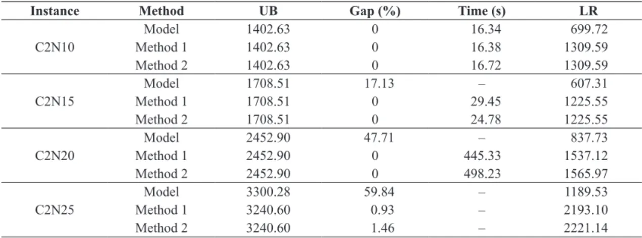
For Case 2, the proposed methods have a better performance compared to the model for instances with up to 25 pairs of pickup and delivery. For instance C2N10, the performance of the three approaches were similar. For instance C2N15, methods 1 and 2 found the optimal solution in a few seconds (approximately 20 seconds), while the model could not prove optimality within 5 hours (17% of relative gap). For C2N20, methods 1 and 2 proved the optimal solution in approximately 450 seconds. The model found an optimal solution, but could not prove its
optimality within 5 hours, inishing with a relative
gap equal to 47%. For C2N25, the model did not
ind the optimal solution in the time limited and
stopped with a 59% of relative gap, while the methods found a better solution with a smaller gap. For other instances, in the time limited, no feasible integer solution was found.
For both cases, the results indicate that the branch-and-cut methods have a better overall performance compared to solving the model directly by the solver. The computational times were better for instances C2N15 and C2N20, in which only the methods were able to prove optimality within the time limit. For instances with more than 30 pairs of pickup and delivery, none of the approaches found feasible solutions within 5 hours of processing time.
Figures 2 and 3 illustrate the routes of two vessels in the optimal solution of C2N25, with Method 1.
Table 2. Computational results for instances of Case 2.
Instance Method UB Gap (%) Time (s) LR
C2N10
Model 1402.63 0 16.34 699.72
Method 1 1402.63 0 16.38 1309.59
Method 2 1402.63 0 16.72 1309.59
C2N15
Model 1708.51 17.13 – 607.31
Method 1 1708.51 0 29.45 1225.55
Method 2 1708.51 0 24.78 1225.55
C2N20
Model 2452.90 47.71 – 837.73
Method 1 2452.90 0 445.33 1537.12
Method 2 2452.90 0 498.23 1565.97
C2N25
Model 3300.28 59.84 – 1189.53
Method 1 3240.60 0.93 – 2193.10
Method 2 3240.60 1.46 – 2221.14
Figure 3. Route of a vessel 24 for instance C2N25 for Method 1.
(projects 2014/22542-2 and 2014/00939-8), CAPES, CNPq and the Agência Nacional de Petróleo (ANP)
for the inancial support.
References
Andersson, H., Hoff, A., Christiansen, M., Hasle, G., & Løkketangen, A. (2010). Industrial aspects and literature survey: Combined inventory management and routing. Computers & Operations Research, 37(9), 1515-1536. http://dx.doi.org/10.1016/j.cor.2009.11.009.
Balas, E., Fischetti, M., & Pulleyblank, W. R. (1995). The precedence-constrained asymmetric travelling salesman polytope. Mathematical Programming, 68(1-3), 214-265. http://dx.doi.org/10.1007/BF01585767.
Baldacci, R., Bartolini, E., & Mingozzi, A. (2011). An exact algorithm for the pickup and delivery problem with time windows. Operations Research, 59(2), 414-426. http://dx.doi.org/10.1287/opre.1100.0881.
Berbeglia, G., Cordeau, J. F., Gribkovskaia, I., & Laporte, G. (2007). Static pickup and delivery problems: a classification scheme and survey. Top, 15(1), 1-31. http://dx.doi.org/10.1007/s11750-007-0009-0.
Brasil. Ministério do Desenvolvimento, Indústria e Comércio Exterior – MDIC. (2011). Recuperado em 30 de abril de 2012, de http://www.mdic.gov.br/sitio/
Brønmo, G., Nygreen, B., & Lysgaard, J. (2010). Column generation approaches to ship scheduling with flexible cargo sizes. European Journal of Operational Research, 200(1), 139-150. http://dx.doi.org/10.1016/j. ejor.2008.12.028.
Christiansen, M. (1999). Decomposition of a combined inventory and time constrained ship routing problem. Transportation Science, 33(1), 1-14. http://dx.doi. org/10.1287/trsc.33.1.3.
Christiansen, M., Fagerholt, K., & Ronen, D. (2004). Ship routing and scheduling: status and perspectives. Transportation Science, 38(1), 1-18. http://dx.doi. org/10.1287/trsc.1030.0036.
Christiansen, M., Fagerholt, K., Ronen, D., & Nygreen, B. (2007). Maritime transportation. In C. Barnhart & G. Laporte (Eds.), Handbook in operations research and management science. Amsterdam: Elsevier. 189-284 p.
Cordeau, J. F. (2006). Branch-and-cut algorithm for the dial-a-ride problem. Operations Research, 54(3), 573-586. http://dx.doi.org/10.1287/opre.1060.0283.
Cordeau, J.-F., Laporte, G., & Ropke, S. (2008). Recent models and algorithms for one-to-one pickup and delivery problems. In B. Golden, S. Raghavan & E. Wasil (Eds.), The vehicle routing problem: latest advances and new challenges (Operations Research/Computer Science Interfaces, 43, pp. 327-357). New York: Springer.
Dantzig, G., & Fulkerson, D. (1954). Minimizing the number of tankers to meet a fixed schedule. Naval
Vessel 14 collects the oil from node 54, delivers it to node 110 and then collects it from platform 48. Nodes 54 and 48 correspond to different platforms, then there is no penalty for consecutive visits. Regarding the route of vessel 24, note that nodes 36, 34, 33 and 35 represent the same platform, but they have different time windows and demands. As in the previous case, there is no cost for consecutive visits for this vessel route.
It should be noted that other branch-and-cut methods were implemented in this study, based on classical two-index models proposed for the PDPTW (Ropke et al., 2007). However, in contrast to the
literature results, these methods were not eficient
with the real instances tested in this paper. The best results were obtained using methods based on the three-index models presented in this paper. Therefore, the other results are not reported.
6 Conclusion
This paper studied the transport of crude oil from offshore platforms to terminals located on the Brazilian coast. A case study was carried out in a Brazilian company that performs this operation, which motivated the proposed mathematical model. The model is based on the classical pickup and delivery problem with time windows, which was extended in order to cover
speciic characteristics of the case study. In addition
to the model, we propose two branch-and-cut methods
with speciic valid inequalities to solve the problem.
The model proposed for the case study involves practical features of the case study, such as multiple
depots, mooring constraints, lexible draft, dynamic
positioning, among others. The proposed branch-and-cut methods were based on variations of this model, including the following valid inequalities: precedence, capacity, subtour elimination, generalized order constraints, infeasible path for time windows, mooring
constraints, lexible draft and dynamic positioning; and
reachability constraints. Computational experiments were conducted with a real data set provided by the company and showed that the branch-and-cut methods obtain better results compared to the model solved directly by a state-of-the-art optimization solver.
As future research, we aim at improving the branch-and-cut methods by including new types of valid inequalities. Another interesting topic would be to develop a branch-and-price method to solve this problem and compare the performance with the branch-and-cut methods proposed in this paper.
Acknowledgements
customers and depot. Journal fur Betriebswirtschaft, 58(1), 21-51. http://dx.doi.org/10.1007/s11301-008-0033-7.
Parragh, S., Doerner, K., & Hartl, R. (2008b). A survey on pickup and delivery problems: Part II: Transportation between pickup and delivery locations. Journal fur Betriebswirtschaft, 58(2), 81-117. http://dx.doi. org/10.1007/s11301-008-0036-4.
Rocha, R., Grossmann, I. E., & Aragão, M. V. S. P. (2009). Petroleum allocation at PETROBRAS: Mathematical model and a solution algorithm. Computers & Chemical Engineering, 33(12), 2123-2133. http://dx.doi.org/10.1016/j. compchemeng.2009.06.017.
Rodrigues, V. P. (2014). Uma abordagem de otimização para a roteirização e programação de navios: um estudo de caso na indústria petrolífera (Dissertação de mestrado). Departamento de Engenharia de Produção, Universidade Federal de São Carlos, São Carlos.
Rodrigues, V. P., Morabito, R., Yamashita, D. S., Silva, B. J., & Ribas, P. C. (2016). Ship routing with pickup and delivery for a maritime oil transportation system: MIP model and heuristics. Systems, 4(3), 31. http://dx.doi. org/10.3390/systems4030031.
Ropke, S., & Cordeau, J. F. (2009). Branch-and-cut and price for the pickup and delivery problem with time windows. Transportation Science, 43(3), 267-286. http://dx.doi.org/10.1287/trsc.1090.0272.
Ropke, S., Cordeau, J. F., & Laporte, G. (2007). Models and branch-and-cut algorithms for pickup and delivery problems with time windows. Networks, 49(4), 258-272. http://dx.doi.org/10.1002/net.20177.
Ruland, K. S., & Rodin, E. Y. (1997). The pickup and delivery problem: Faces and branch-and-cut algorithm. Computers & Mathematics with Applications, 33(12), 1-13. http://dx.doi.org/10.1016/S0898-1221(97)00090-4.
Savelsbergh, M. W. P., & Sol, M. (1995). The general pickup and delivery problem. Transportation Science, 29(1), 17-29. http://dx.doi.org/10.1287/trsc.29.1.17.
Sherali, H., Al-Yakoob, S., & Hassan, M. (1999). Fleet management models and algorithms for an oil-tanker routing and scheduling problem. IIE Transactions, 31(5), 395-406. http://dx.doi.org/10.1080/07408179908969843.
Stålhane, M., Andersson, H., Christiansen, M., Cordeau, J.-F., & Desaulniers, G. (2012). A branch-price-and-cut method for a ship routing and scheduling problem with split loads. Computers & Operations Research, 39(12), 3361-3375. http://dx.doi.org/10.1016/j.cor.2012.04.021. Research Logistics Quarterly, 1(3), 217-222. http://
dx.doi.org/10.1002/nav.3800010309.
Desaulniers, G., Desrosiers, J., Erdmann, A., & Solomon, M. M. (2002). VRP with pickup and delivery. In P. Toth & D. Vigo (Eds.), The vehicle routing problem (pp. 225-242). Philadelphia: Society for Industrial and Applied Mathematics.
Dumas, Y., Desrosiers, J., & Soumis, F. (1991). The pickup and delivery problem with time windows. European Journal of Operational Research, 54(1), 7-22. http:// dx.doi.org/10.1016/0377-2217(91)90319-Q.
Fagerholt, K., & Ronen, D. (2013). Bulk ship routing and scheduling: solving practical problems may provide better results. Maritime Policy & Management, 40(1), 48-64. http://dx.doi.org/10.1080/03088839.2012.744481.
Fisher, M. L., & Jaikumar, R. (1981). A generalized assignment heuristic for vehicle routing. Networks, 11(2), 109-124. http://dx.doi.org/10.1002/net.3230110205.
Hennig, F., Nygreen, B., Christiansen, M., Fagerholt, K., Furman, K. C., Song, J., Kocis, G. R., & Warrick, P. (2012). Maritime crude oil transportation - a split pickup and split delivery problem. European Journal of Operational Research, 218(3), 764-774. http://dx.doi. org/10.1016/j.ejor.2011.09.046.
Hoff, A., Andersson, H., Christiansen, M., Hasle, G., & Løkketangen, A. (2010). Industrial aspects and literature survey: fleet composition and routing. Computers & Operations Research, 37(12), 2041-2061. http://dx.doi. org/10.1016/j.cor.2010.03.015.
Hwang, H., Visoldilokpun, S., & Rosenberger, J. M. (2008). A branch-and-price-and-cut method for ship scheduling with limited risk. Transportation Science, 42(3), 336-351. http://dx.doi.org/10.1287/trsc.1070.0218.
Lu, Q., & Dessouky, M. (2004). An exact algorithm for the multiple vehicle pickup and delivery problem. Transportation Science, 38(4), 503-514. http://dx.doi. org/10.1287/trsc.1030.0040.
Lysgaard, J. (2006). Reachability cuts for the vehicle routing problem with time windows. European Journal of Operational Research, 175(1), 210-223. http://dx.doi. org/10.1016/j.ejor.2005.04.022.
Nowak, M., Ergun, O., & White, C. C. 3rd (2008). Pickup and delivery with split loads. Transportation Science, 42(1), 32-43. http://dx.doi.org/10.1287/trsc.1070.0207.