Journal of Applied Fluid Mechanics, Vol. 9, No. 3, pp. 1157-1166, 2016. Available online at www.jafmonline.net, ISSN 1735-3572, EISSN 1735-3645.
Time Response of Natural Convection of Nanofluid
CuO-H
2
O in Enclosure Submitted to a Sinusoidal Thermal
Boundary Condition
M. Bouhalleb
1†and H. Abbassi
21
Unit of Computational Fluid Dynamics and Transfer Phenomena
2
National Engineering School of Sfax.BP1173,3038 sfax, University of Sfax, TUNISIA
†Corresponding Author Email: [email protected]
(Received November 15, 2014; accepted June 4, 2015)
A
BSTRACTA two-dimensional steady laminar natural convection in rectangular enclosure filled with CuO-water nanofluid is numerically investigated. The horizontal walls are thermally insulated and the left vertical side one is heated by a temporal sinusoidal temperature variation, whereas the right wall is kept at cold temperature. Mass Conservation, momentum, and energy equations are numerically solved by the finite volume element method using the SIMPLER algorithm for pressure-velocity coupling. This study has been carried out for four parameters: the volumetric fraction of nanoparticles (0%≤≤4%), aspect ratio Ar (0.25≤Ar≤1), amplitude of temperature a (0.2≤a≤0.8) and its period (0.2≤Θ≤0.8). These simulations are performed at constant Rayleigh and Prandtl numbers (Ra=105and Pr=7.02). Numerical results show that the addition of nanoparticules into the basic fluid has a double role, increasing heat transfer and reducing the response time of the system. The decreasing of aspect ratio shows an increasing trend of the heat transfer and increases the amplitude of Nusselt number. We also see that after a time period the system does not return to its initial state (hysteresis phenomenon) because of the system inertia.
Keywords: Nanofluid; Nanoparticules; Time response; Aspect ratio; Period.
1.
INTRODUCTION
Natural-convection flows generated by buoyancy forces in rectangular closed cavities have been the subject of numerous studies in the past. Actually, considerable efforts are still devoted in the area, where this basic geometry remains still attractive. The interest in such problems stems from their importance in many engineering applications such as convective heat loss from solar collectors, thermal design of buildings, air conditioning, and recently, the cooling of electronic components and many other applications. In fact, in practical applications involving natural convection as a removal heat transfer mechanism, the energy provided to the system is variable in time and gives rise to unsteady natural convection flow. Solar collectors and printed circuit boards are examples of such systems submitted to variable thermal boundary conditions. Moreover, by an appropriate choice of the parameters characterizing the variable excitation (amplitude and period of a periodic heating or cooling temperature, for example), it becomes possible to establish a variety of dynamical regimes (periodic, quasi-periodic, intermittent, chaotic etc.) instead of a stationary
regime. In an earlier investigation, Lage and Bejan (1993) numerically and theoretically studied the problem of natural convection in enclosures with one side heated with a pulsating heat flux. They showed that the buoyancy-induced flow resonates to a certain frequency of the pulsating heat input and the resonance phenomenon is characterized by maximum fluctuations observed in the heat transfer evolution with the time-depending temperature period. M. Kazmierczak and Z. Chinoda 1992 studied the unsteady
Buoyancy-driven flow in an enclosure with time periodic boundary conditions, they showed that increasing the amplitude or the period of the hot wall temperature oscillation increased the cycle-averaged heat transfer only slightly.
Antohe and Lage (1996) theoretically and numerically investigated the case of clear fluid and fully saturated porous medium differentially heated enclosures with a time periodic pulsating heat flux. The numerical simulations indicate that the natural convection activity within the enclosure reaches several local maxima for certain values of the heating frequency referred to as resonance frequency.
Finally, it is interesting to underline that the imposition of boundary conditions periodically varies with allocated time, by means of an appropriate choice of the control parameters, to suppress the chaos in some conditions where it normally exists, as reported by Lima and Pettini (1990) and Kim and Stringer (1992), or to establish it were not existing, as reported by Xia et al. (1995). These possibilities, offered by variable heating conditions, could be properly exploited according to the application needs.
Sarris et al. (2002) numerically investigated natural convection in air-filled rectangular enclosure with sinusoidal temperature profile on the upper wall and adiabatic conditions on the bottom and sidewalls. Results of the study show that, the thermal boundary layer is formed on the upper wall with its thickness decreases while as the Rayleigh number increases. This results in a lower temperature penetration depth and may have important implications in the design of glass melting tanks. Increasing the tank aspect ratio increases the fluid circulation intensity and the thermal penetration depth, which are important parameters for improving glass melt homogenization. Basak et al. 2006 performed a numerical study on laminar natural convection in an air-filled square cavity with uniformly and non-uniformly heated bottom wall, and adiabatic top wall maintaining constant temperature of cold vertical walls. The results show that the non-uniform heating exhibits greater heat transfer rates than that with uniform heating for all Rayleigh numbers. Bilgen and Yedder (2007) carried out a numerical study on natural convection of air in rectangular enclosures with sinusoidal temperature profiles on side walls and insulated other ones. The results show that the thermal penetration is a function of the aspect ratio and Rayleigh number. Generally, it approaches to 100% at high Rayleigh numbers when the lower half is heated and the upper half cooled. Results of a numerical study on natural convection in an air-filled rectangular enclosure with linear temperature distributions on both side walls were reported by Sathiyamoorthy et al. (2007). Sivasankaran et al. 2010 conducted a numerical study on mixed convection in a lid-driven cavity with sinusoidal temperature distribution on side walls, and moving adiabatic top wall. The results show that, when the amplitude of temperature increases, the heat transfer also increases in the natural convection regime. As the velocity of fluid is increases as the Richardson number and amplitude ratio increases too. In another numerical study, Sivasankaran et al. (2011) investigated the effects of a magnetic field on mixed convection inside a lid-driven square cavity
with sinusoidal temperature profiles on side walls. They showed that when the left sidewall is kept with sinusoidal temperature distribution, the heat transfer increases and so does the amplitude ratio.
Most of the studies are performed in square enclosures. However, natural convection is very important in other geometries in real life situations, particularly, rectangular enclosures. Wilkes and Churchill 1966 performed a finite difference computation on natural convection in a long horizontal rectangular enclosure. They demonstrated that the steady state results are in good agreement with analytical solutions. The effect of aspect ratio on natural convection of nanofluid was studied by Tong (1999). The results revealed that Nusselt number exhibits a strong dependence on aspect ratio (Ar), Ra and the density distribution of nanoparticles.
In some heat transfer applications, nano-sized particles (average particle size less than 100 nm) are added in the base fluid such as water or ethylene glycol to obtain better thermal properties compared to base flow. Nanofluids have improved heat transfer characteristics with little pressure drop as compared to base fluids (Oztop and Abu-Nada 2008).
The literature review showed that nanofluids lead to improvement in the heat transfer performance, which is in a good agreement with experimental works. Modifications could be made to achieve more accurate results from numerical processes. Shahi et al. 2010 have numerically investigated the convective cooling in a square vented cavity and partially heated from below utilizing nanofluids. They showed that increase in solid concentration leads to increase in the average Nusselt number at the heat source surface and decrease in the average bulk temperature.
performance. The nanofluid was a mixture of pure water and nanoscale Cu particles at various volume fractions. Due to the increased thermal conductivity and thermal dispersion effects, they found that performance was greatly improved when nanofluids were used as a coolant. In addition, they observed that the presence of nanoparticles in the fluid did not produce any extra pressure drop because of small particle size and low particle volume fraction.
2.
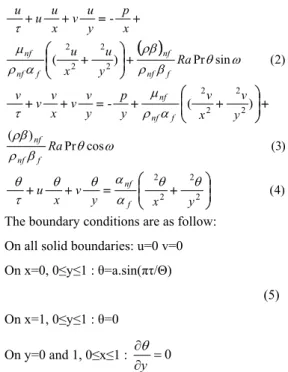
STATEMENT OF THE PROBLEMThe geometry of the studied problem is shown in Fig. 1. It consists of a two-dimensional cavity with height H and length L filled with mixture of water and solid particles CuO. The left wall of the enclosure is heated with a temperature varying sinusoidally in time (TC+a.sin(πt/Θ), while the vertical right wall is cooled at a constant temperature Tc. The horizontal walls are assumed to be insulated and impermeable to mass transfer. The nanofluid in the cavity is supposed to be Newtonian, incompressible and the flow is supposed to be laminar. Thermophysical properties of water and nanoparticle (CuO) are assumed to be constant (table 1). The density of the nanofluid is supposed to be constant except in the buoyancy term where boussinesq approximation is imposed.
Fig. 1- Schematic diagram.
Table 1 Physical Properties of Pure Water and Cuo Solid Particle
(kg m-3)
Cp (Jkg-1 K-1)
k (Wm-1K-1)
(k-1) Pure
water
997.1 4179 0.613 2.110-4
CuO
6320 531.8 76.5 1.810-5
3.
MATHEMATICAL FORMULATIONBy the law of mass conservation, momentum and energy, the governing equations are:
) 1 ( 0 y v x u
) 2 ( sin Pr ) ( -2 2 2 2 Ra y u x u x p y u v x u u u f nf nf f nf nf ) 3 ( cos Pr ) ( ) ( -2 2 2 2 Ra y v x v y p y v v x v v v f nf nf f nf nf ) 4 ( 2 2 2 2 y x y v x u fnf
The boundary conditions are as follow:
On all solid boundaries: u=0 v=0
On x=0, 0≤y≤1 : θ=a.sin(πτ/Θ)
(5)
On x=1, 0≤y≤1 : θ=0
On y=0 and 1, 0≤x≤1 : 0 y
The expressions of density, specific heat, thermal expansion coefficient and dynamic viscosity of the nanofluid are given as follows Chein et al 2009:
(1- )
nf f s
(6) (Cp nf) (1- )( Cp f) (Cp s)
(7) ()nf (1- )( )f ( )s
(8) 2.5 (1- ) f nf
(9)
The local Nusselt number Nu(x) can be expressed as: ) 0 1 ( x k k ) y ( Nu 1 x f eff
Effective conductivity
k
effof the nanofluid iscalculated as follows Koo et al 2004:
eff stat brow
k k k
(11)
The static conductivity
k
stat is given by the Maxwell model Maxwell et al 1904:2 2( - )
2 -( - )
s f s f
stat f
s f s f
k k k k
k k
k k k k
(12)
The Brownian conductivity is formulated as (Koo and Kleinstreuer 2004):
4 1
5 10 ( , )
brow f pf
s s T
k C f T
d
(13)
Where sand ds are the density and the diameter of nanoparticles, respectively and is the
Boltzmann constant 1.3807 10 23J/K . For the water-CuO nanofluid, the two modeling functions 1 and f are experimentally estimated
as :
0.7272 1 0.0011(100 )
for
1
٪
,
( 6.04 0.4705) (1722.3 134.63)f T
T
for 1
٪
4٪
The total heat transferred from the hot wall to the flow is evaluated by the space averaged Nusselt number expressed as
0 1
( ) (14)
A r
Nu Nu y dy
A r
4.
NUMERICAL METHODOLOGYA modified version of Control Volume Finite-Element Method (CVFEM) of Saabas and Baliga (1994) is adapted to the standard staggered grid in which pressure and velocity components are stored at different points. The SIMPLER algorithm of Patankar 1980 was applied to resolve the pressure-velocity coupling in conjunction with an Alternating Direction Implicit (ADI) scheme for performing the time evolution. The numerical code used here is described and validated in details in Abbassi et al. (2001a, 2001b).The conditions necessary to prevent numerical instabilities are determined from a combination of Courant– Friedrichs–Lewy (CFL) conditions and the restrictions on the grid Fourier number. According to the CFL conditions, the distance the fluid travels in one time increment must be less than one space increment (∆x or ∆y), and lead to a constraint on the time step ∆τ:
; x y u v
(15)
From this condition, the used grid and velocity
fields, the time step is limited by1.57 10 -4. In the following computations is fixed at 10-5.
5.
GRID REFINEMENT AND TESTVALIDATION
Grid refinement tests have been performed for four uniform grids: 51×51, 6161, 71×71 and 81×81 for Ra=105, =4% and Ar=1 applied to configuration of our problem. Results show that when we moved from the first grid to the second, the Nusselt number (Nu) moved from 3.1447 to 3.1185, undergoing a variation of 0.84%. When we moved from the second grid to the third, the Nusselt number becomes 3.1030, undergoing a decrease of 0.50%. Now, when we moved from the third grid to the fourth, the Nusselt number becomes 3.0952, undergoing a decrease of only 0.25%. We conclude that the grid of 71×71 is sufficient to carry out the numerical study of this flow. A particular care is taken when varying the aspect ratio; the grid is extended or reduced keeping constant space steps.
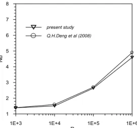
The present code was also tested to simulate the case studied by Qi-Hong Deng and Juan-Juan Chang (2008). We calculated the average Nusselt number for the rectangular enclosure with sinusoidal space temperature distributions on the left side wall at Pr=0.71 and for various Rayleigh numbers. As can be seen from Fig 2, the results predicted by current computer code agree well with the previous study.
Fig. 2. Test validation: Comparisons with Qi-Hang Deng and Juan-Juan Chang (2008) with
Pr=0.71 and Ar=1.
Present study
Deng and Chang (2008)
Sivasankaran and Bhuvaneswari (2013)
Fig. 3. Comparison of the present results with Deng and Chang (2008) and Sivasankaran and
Bhuvaneswari (2013).
0.00 0.10 0.20 0.30 0.40 0.50 0.60 0.70 0.80 0.90 1.00 0.10
0.20 0.30 0.40 0.50 0.60 0.70 0.80 0.90 1.00
0 00 0 10 0 20 0 30 0 40 0 50 0 60 0 70 0 80 0 90 1 00 0.10
0.20 0.30 0.40 0.50 0.60 0.70 0.80 0.90 1.00
1E+3 1E+4 1E+5 1E+6
Ra 1
2 3 4 5 6 7 8
Nu
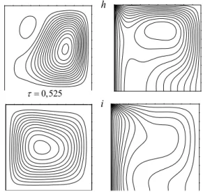
Fig. 4. Streamlines and isotherms in a flow cycle for different times with Ra=105 a=1, =2℅,
Θ=0.5 and Ar=1.0.
6.
RESULTS AND DISCUSSIONS6.1
Time evolution of Thermal and
Dynamic Fields
In many physical situations, we seek to study
the response of a system to an external
excitation. This article presents a study of the
dynamic response of an excited thermal
system.
The results and their analysis are given below
for specific sinusoidal excitation imposed at
the left side of the enclosure.
The main parameters governing the present
problem are the volume fraction (0
℅≤
≤
2
℅
),
the aspect ratio (0.25
≤
Ar
≤
1), the period
(0.01
≤Θ≤
0.8) the amplitude (0.2
≤
a
≤
1). The
Prandtl and Rayleigh numbers values were
maintained constant at 7.06 and 10
5,
respectively. In the following, the results
obtained are first presented as streamlines and
isotherms, in order to learn how the system
replies once exited with a temperature
periodically varying with time.
In figures 4a-4i, the effect of the variable
heating at different times on the dynamical,
thermal and heat transfer behaviours of the
fluid is illustrated by presenting streamlines
and isotherms over slightly more than one
cycle flow.
The streamline plots of this figure show that
the flow field is dominated by a primary large
cell filling most of the cavity rotating in a
clockwise direction, then, it appears a weak
small secondary cell rotating in the counter
clockwise direction.
a
b
c
d
0
0.05
0.125
2
e
0, 47
f
0, 485
g
h
0,525
i
0,545
We note that for the beginning, we observed
that the flow main dominant is formed by only
one cell rotating in the clockwise sense with
an inactive area located close of the right cold
wall of the enclosure. The cell centre is
positioned toward the hot wall side of the
enclosure.
Once the time increases to reach 0.125, the
recirculation cell will shift toward to the right.
The inactive area is reduced and the flow
remains unicellular. At
τ
=
Θ
/2 the central cell
takes an elliptical shape, and the centre of the
cell is in the middle of the enclosure.
A secondary cell appears at
τ
=0.485 (fig.4(f))
similar to that found by M. kazmierczak et al
(1992), this secondary cell grows in size and
intensity (Figs. 4(g)) over the second half of
the time period of the hot wall temperature
variation where the instantaneous hot wall
temperature is always less than the average
value. Continuing further in time, the region of
secondary recirculation greatly decreases in
size then totally disappears as
τ
=0.545 (Fig.
4(i)).
During the second half of the cycle,
simultaneously with the appearance of the
secondary flow, the flow intensity in the main
cell is much weaker, the maximum stream
function
ψ
maxin the main cell, decreases as
time increases (
ψ
max=11.00 for
τ
=0.47 and
ψ
max=7.00 for
τ
=0.5) and its location has
shifts toward the vertical cold wall.
As regards the isotherms and during the
time when the hot wall temperature is
increasing (Figs. 4(a)-(d)), a well defined
thermal boundary layer is visible on left
vertical wall. However, when the hot wall left
temperature decreases the thermal boundary
layer on the left hot wall moves to the right
wall.
6.2
Heat Transfer Under the Effect of
Nanofluid Concentration
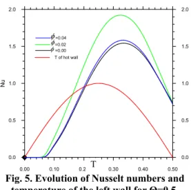
Figure.5 shows the time evolution of the
average Nusselt number (
Nu
) for different
values of volume fraction, together with the
variation of temperature at the left boundary.
At the beginning, Nu is typically zero,
indicating that heat does not reach the right
wall; therefore the system begins to respond
after a finite time delay. After this time the
Nusselt number will go up very quickly, it
reaches a maximum value and then, gradually
decreases. In fact the increase of the volume
fraction is accompanied by proportional
increase in the amplitude of Nusselt number
up to
φ
=2% and decreases for
φ
=4% but
remains superior to
φ
=0% (fig.5) similar to
reference Fatih
et al
. (2013). We note that after
excitation by a sinusoidal temperature, the
response time (
τ
resp) of the system decreases by
increasing the volume fraction of
nanoparticules. For
=0%, the response time
τ
resp=0.044, when
=2%
τ
resp=0.033. For
=4% the response time increases, but remains
below 0%. We can conclude that the system
response time decreases with the increase of
volume fraction, indicating that the fluid
thermal conductivity becomes more important
to the presence of nanoparticles.
Fig. 5. Evolution of Nusselt numbers and
temperature of the left wall for
Θ
=0.5.
Table 2 shows the temporal gap between the
time of the maximum temperature and the time
of maximum Nusselt number, for different
volume fraction values. We define by
τ
max
the time corresponding to the maximum
amplitude, the gap is used to measure the
quality of the response. As expected, the
addition of solid particles improves the
response of system and reduces significantly
the time gap.
Δτ
decreases remarkably with
increasing
reaching a minimum at
=2%
and then increasing slowly but remaining
inferior to the case of pure water. The decrease
of temporal gap due to solid particle addition
up to 2
℅
CuO concentration reaches 17.6%.
Table 2 Temporal Gap for Different Values of Volume Fraction
0% 1% 2% 3% 4%
τmax 0.335 0.325 0.320 0.324 0.332 Τ
(Tmax(hot wall)) 0.25 0.25 0.25 0.25 0.25 Δτ=
(τmax-τ(Tmax)) 0.085 0.075 0.07 0.074 0.082
Figure.6 illustrates the effect of the volume
fraction on vertical velocities for pure water as
well as the CuO-water nanofluid at the
midsection of the enclosure. There is a
0.00 0.10 0.20 0.30 0.40 0.50 0.0
0.5 1.0 1.5 2.0
Nu
0.0 0.5 1.0 1.5 2.0
T of hot wall =0.00 =0.02 =0.04
difference for velocity profiles between the
zero volume fraction and the other volume
fractions. This difference is related to adding
the nanoparticles into the fluid associated
random through the fluid which in turn results
in higher velocity for the nanofluid.
Fig. 6. Velocity profiles for different concentrations at y=0.5, Ar=1, τ=0.5, a=1 and
Θ=0.5.
6.3
Effect of Aspect Ratio
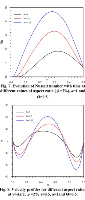
Figure 7 presented the Nusselt number and
their evolutions for different aspect ratios. The
results presented put in evidence an obvious
effect of aspect ratio (
Ar
) on the amplitude of
Nu
. In the range 0.25
≤
Ar
≤
1 the amplitude of
Nusselt number undergoes a significant
increase when Ar decreases. For all aspect
ratio and applied with the heated portion, one
periodic excitation temperature, the heat
transfer value increases to reach a maximum
value and decreases. This value is reached at
different times (
τ
max),
τ
maxdecreases with
decreasing aspect ratio. For
Ar
=1
τ
max=0.3247,
Ar=0.5
τ
max=0.2987 and
Ar
=0.25
τ
max=0.2848.
We notice that after excitation by a sinusoidal
temperature, the response time (
τ
resp) of the
system decreases by decreasing the aspect
ratio. For example for
Ar
=1,
τ
resp=0.033, when
Ar
=0.5,
τ
resp=0.011, therefore the system
becomes three times quicker than Ar=1. For
Ar
=0.25,
τ
resp=0.005, the system is seven times
quicker compared to
Ar
=1. We can conclude
that the system response time decreases with
the decrease of the aspect ratio, indicating that
the speed of fluid flow becomes more
important to the aspect ratio decrease.
We also note that after a flow cycle (period)
the system does not return to its ground state
and this is due to the system inertia that can
store the generated energy.
Fig.8 shows the variation of vertical velocity
component profiles along the horizontal line
passing by the geometrical centre of the
enclosure for three aspect ratios
Ar
=1,
Ar
=0.5
and
Ar
=0.25. It is found for a rectangular
enclosure that when aspect ratio increases, the
fluid velocity increases.
Fig. 7. Evolution of Nusselt number with time at different values of aspect ratio (=2℅), a=1 and
Θ=0.5.
Fig. 8. Velocity profiles for different aspect ratios
at y=Ar/2, =2% τ=0.5, a=1and Θ=0.5.
6.4
Effect of Amplitude and Period
The effect of the amplitude of sinusoidal
boundary temperature on the temporal
variations of nusselt number Nu(
τ
), are
presented in fig.9. The figure zoom, represents
the response of system for different values of
amplitude of temperature at the left side wall.
The variation of Nusselt number is
characterized by increasing amplitudes
following the increase of (a). We also note that
after excitation the system response time
decreases with the amplitude increase, for
(a=0.2,
τ
resp=0.0408), (a=0.4,
τ
resp=0.0367),
0.0 0.2 0.4 0.6 0.8 1.0
x
-45 -30 -15 0 15 30
V
=0.04
=0.02
=0.00
0.0 0.1 0.2 0.3 0.4 0.5
0 1 2 3 4 5
Nu
Ar=1
Ar=0.5
Ar=0.25
0.0 0.2 0.4 0.6 0.8 1.0
X
-90 -60 -30 0 30 60 90
V
Ar=1
Ar=0.5
Ar=0.25
(a=0.6,
τ
resp=0.0349),(a=0.8,
τ
resp=0.034),(a=1.0,
τ
resp=0.0330).We spend from the a=0.2 to a=1,
the decrease of the response times of the
system reaches 19%. As for the time of
maximum amplitude of
Nu
, it decreases with
the amplitude increase (a).
Fig. 9. Effect of the amplitude on the variation of Nusselt number in function with time, with Ar=1,
=2℅ and Θ=0.5.
Fig. 10. Velocity profiles for different amplitude at y=0.5, Ar =1, Θ=0.5 and τ=0.5.
Fig.10 illustrates the effect of amplitude (
a
) on
the horizontal velocity. There is a significant
difference for velocity profile between
a
=0.2
and
a
=1. The velocity is increasing with
amplitude (
a
) increasing. We note that in the
case where the amplitude of the temperature is
equal to 0.2, the Nusselt number at the lower
intensity, relative to other amplitude (fig.9)
and this is due to the low velocity encountered
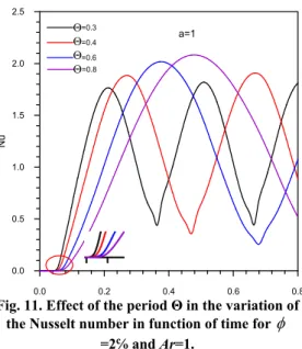
at this amplitude (a=0.2). The effect of the
period on the temporal variation of Nusselt
number is illustrated in fig.11 for a=1 and
different values of
Θ
. In this case, the
sinusoidal nature of excitation is relatively
well reproduced in the temporal variation of
this quantity Nu(
τ
). We note that the
amplitudes of the oscillations of the Nusselt
number increases when
Θ
increases. We can
clearly observe that the increase in the period,
fact increased the time required for the system
response as clearly indicated by the zoom. In
fact, in the figure.4 and for various values of
τ
,
the important changes in the flow structure are
obtained with the low values of the period
particularly for
Θ
=0.5. However, when the
system is excited with low imposed
frequencies, it rapidly replies as shown in the
above figure. With increasing the period, heat
transfer is enhanced.
Fig. 11. Effect of the period Θ in the variation of the Nusselt number in function of time for
=2℅ and Ar=1.
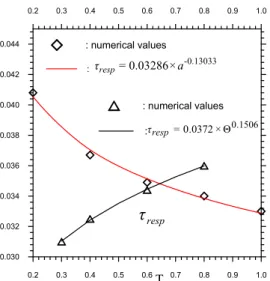
6.5
Correlations for Time Response
Figure 12 summarizes the time response
variation in function of the amplitude (
a)
and
period
Θ
. As can be seen,
τ
respdecreases, as (
a
)
increases, but
τ
respincreases with increasing
the period. The behavior of this decrease can
be modeled by a power low:
τresp=α×aβ (16)
The smoothing by least square method shows
that:
α
= 0.03286 and
β
=-0.13033
And the increase of
τ
respas a function of the
period is modeled by:
τ
resp=
α
1×
Θ
β1 (17)The smoothing by least square method shows
that:
α
1= 0.03721 and
β
1=0.15060
Figure 12 shows also that the proposed model
agrees well with numerical results, the
maximum deviation is less than 3% for
τ
respas
0.0 0.1 0.2 0.3 0.4 0.5 0.0
0.5 1.0 1.5 2.0
Nu
a=0.2
a=0.4
a=0.6
a=0.8
a=1
0.0 0.2 0.4 0.6 0.8 1.0 x
-45 -30 -15 0 15 30
V a=0.2
a=0.4
a=0.6
a=0.8
a=1
0.0 0.2 0.4 0.6 0.8 0.0
0.5 1.0 1.5 2.0 2.5
Nu
=0.3 =0.4 =0.6
a=1
=0.8
T
a function of amplitude, and in the order of
0.27% for
τ
respas a function of period.
Fig. 12. Response time as a function of the amplitude and the period of temperature.
7.
CONCLUSIONThe natural convection in a rectangular enclosure with temporal sinusoidal temperature variation on one side wall has been numerically studied. The coupled non linear equations of momentum and energy including buoyancy forces under the Boussinesq approximation are numerically solved. From the study, the following conclusions are drawn:
1. The system response time decreases by increasing the volume fraction of solid particles. 2. The volume fraction increase is accompanied by proportional increase in the amplitude of Nusselt number.
3. The amplitude of Nusselt number undergoes a significant increase when Ar decreases.
4. The system responds quickly, when increasing the amplitude of temperature excitation.
5. When the system is excited with low imposed frequencies, it rapidly replies.
6. When the aspect ratio increases, the system response time increases.
R
EFERENCESAbbassi, H. S., S. Turki and B. Nasrallah (2001). Mixed convection in a plane channel with a built-in triangular prism. Numer. Heat Transfer A 39(3), 307–320.
Abbassi, H. S., S. Turki and B. Nasrallah (2001). Numerical investigation of forced convection in a plane channel with a built-in triangular prism. Internat. J. Thermol. Sci. 40, 649–658.
Antohe, B. V. and J. L. Lage (1996). Amplitude Effect on Convection Induced by Time-Periodic, horizontal Heating. Int. J. Heat Mass Transfer. 39, 1121–1133.
Bilgen, W. and R. B. Yedder (2007). Natural convection in enclosure with heating and cooling by sinusoidal temperature profiles on one side. International Journal of Heat and Mass Transfer 50, 139–150.
Chein, R. and G. Huang (2005). Analysis of Microchannel Heat Sink Performance Using Nanofluids. Applied Thermal Engineering. 25, 3104–3114.
Deng, Q. H. and J. J. Chang (2008). Natural Convection in a Rectangular Enclosure with Sinusoidal Temperature Distributions on Both Side Walls. Numer. Heat Transfer A 54, 507– 524.
Douamna, S., M. Hasnaoui and B. Abourida (2000). Two-Dimensional Transient Natural Convection in a Repetitive Geometry Submitted to Variable Heating From Below. Numerical Identification of Routes Leading to Chaos. Numer. Heat Transfer A 37, 779–799.
Fatih, S. and H. F. Öztop (2013). Identification of forced convection in pulsating flow at a backward facing step with a stationary cylinder subjected to nanofluid. International Communications in Heat and Mass Transfer 45 111–121.
Gosselin, L. and A. K. Da Silva (2004). Combined Heat Transfer and Power Dissipation Optimization of Nanofluid Flows. Applied Physics Letters 85(18), 4160–4162,.
Kazmierczak, M. and Z. chinoda (1992). Compact Buoyancy-driven flow in an enclosure with time periodic boundary conditions. Int. J. Heat Mass Transfer 35(6), 1507-1518.
Kim, J. H. and J. Stringer (1992). Applied Chaos, Wiley, New York.
Koo, J. and C. Kleinstreuer (2004). A new thermal conductivity model for nanofluids. J Nanoparticle Res 6, 577-88.
Lage, J. L. and A. Bejan (1993). The Resonance of Natural Convection in a Horizontal Enclosure Heated Periodically from the Side. Int. J. Heat Mass Transfer 36, 2027–2038.
Lima, R. and M. Pettini (1990). Suppression of Chaos by Resonant Parametric Perturbations. Phys. Rev. A 41, 726–733.
Maxwell J. (1904). A treatise on electricity and magnetism. 2nd ed. Oxford. Cambridge: University Press 435-41
Oztop, H. F. and E. Abu-Nada (2008). Numerical study of natural convection in partially heated rectangular enclosures filled with nanofluids. International Journal of Heat and Fluid Flow 29, 1326–1336.
Patankar, S. V. (1980). Numerical heat transfer and fluid flow. Washington, D. C.: Hemisphere Publishing Corporation 113-37.
Roy, T. S. and A. R. Balakrishnan (2006). Effects 0.2 0.3 0.4 0.5 0.6 0.7 0.8 0.9 1.0
0.030 0.032 0.034 0.036 0.038 0.040 0.042 0.044
0.2 0.3 0.4 0.5 0.6 0.7 0.8 0.9 1.0
: numerical values
:
: numerical values
: τresp=0.0372×Θ0.1506 13033 . 0
-× 03286 . 0
= a
τresp
resp
τ
of thermal boundary conditions on natural convection flows within a square cavity. International Journal of Heat and Mass Transfer 49, 4525–4535.
Sivasankaran, S. A. Malleswaran, J. Lee and P. Sundar (2011). Hydro-magnetic combined convection in a lid-driven cavity with sinusoidal boundary conditions on both sidewalls. International Journal of Heat and Mass Transfer 54, 512–525.
Saabas, H. J., and B. R. Baliga (1994). Co-located equal-order control-volume finite-element method for multidimensional, incompressible, fluid flow part I: formulation. Numer Heat Transf Part B, 26, 409-24.
Sarris, I. E., I. Lekakis and N. S. Vlachos (2002). Natural Convection in a 2D enclosure with sinusoidal upper wall temperature. Numerical Heat Transfer Part A 42, 513–530.
Sathiyamoorthy, M., T. Basak, S. Roy and I. Pop (2007). Steady natural convection flows in a square cavity with linearly heated side wall(s). International Journal of Heat and Mass Transfer 50, 766–775.
Shahi, M. A., H. Mahmoudi and F. Talebi (2010). Numerical study of mixed convective cooling in a square cavity ventilated and partially heated from the below utilizing nanofluid.
International Communications in Heat and Mass Transfer 37 201–213.
Sivasankaran, S. and M. Bhuvaneswari (2013). natural convection in a porous cavity with sinusoidal heating on both sidewalls. Numerical Heat Transfer Part A 63, 14–30.
Sivasankaran, S., V. Sivakumar and P. Prakash (2010). Numerical study on mixed convection in a lid-driven cavity with non-uniform heating on both sidewalls. International Journal of Heat and Mass Transfer 53, 4304–4315.
Tong, W. (1999). Aspect ratio effect on natural convection in water near its density maximum temperature. International Journal of Heat and Fluid Flow 20, 624–633.
Tzeng, S. C., C. W. Lin and K. D. Huang (2005). Heat Transfer Enhancement of Nanofluids in Rotary Blade Coupling of Four- Wheel-Drive Vehicles. Acta Mechanica 179, 11–23.
Wilkes, J. O. and S. W. Churchill (1966). The finite-difference computation of natural convection in a rectangular enclosure. AIChE Journal 12(1), 161–166.