REGRESSION EQUATIONS BETWEEN BODY AND HEAD
MEASUREMENTS IN THE BROAD-SNOUTED CAIMAN
(Caiman latirostris)
VERDADE, L. M.
Laboratório de Ecologia Animal, ESALQ, Universidade de São Paulo, C.P. 09, CEP 13418-900, Piracicaba, SP, Brazil
Correspondence to: Luciano M. Verdade, Laboratório de Ecologia Animal, ESALQ, Universidade de São Paulo, C.P. 09, CEP 13418-900, Piracicaba, SP, Brazil, e-mail: [email protected]
Received March 4, 1999 – Accepted December 22, 1999 – Distributed August 31, 2000
(With 5 figures)
ABSTRACT
In the present study, regression equations between body and head length measurements for the
broad-snouted caiman (Caiman latirostris) are presented. Age and sex are discussed as sources of
varia-tion for allometric models. Four body-length, fourteen head-length, and ten ratio variables were taken from wild and captive animals. With the exception of body mass, log-transformation did not improve the regression equations. Besides helping to estimate body-size from head dimensions, the regres-sion equations stressed skull shape changes during the ontogenetic process. All age-dependent variables are also size-dependent (and consequently dependent on growth rate), which is possibly related to the difficulty in predicting age of crocodilians based on single variable growth curves. Sexual dimor-phism was detected in the allometric growth of cranium but not in the mandible, which may be evo-lutionarily related to the visual recognition of gender when individuals exhibit only the top of their heads above the surface of the water, a usual crocodilian behavior.
Key words: relative growth, sexual dimorphism, size estimates, broad-snouted caiman, Caiman latirostris.
RESUMO
Equações de regressão entre medidas de corpo e cabeça em jacarés-de-papo-amarelo
(Caiman latirostris)
No presente estudo, equações de regressão entre medidas de comprimento do corpo e cabeça de
jacarés-de-papo-amarelo (Caiman latirostris) são apresentadas. Idade e sexo são discutidos como fontes de
variação para modelos alométricos. Quatro medidas de comprimento corpóreo, 14 medidas de com-primento da cabeça e dez proporções relativas entre medidas foram tomadas de animais selvagens e cativos. Com excessão da massa corpórea, a transformação logarítmica não incrementou as equações de regressão. Além de auxiliar na estimativa do comprimento corpóreo a partir de dimensões da cabeça, as equações de regressão evidenciaram alterações na forma craniana durante processos ontogênicos. Todas as variáveis dependentes da idade mostraram-se também dependentes do tamanho (e conseqüentemente da taxa de crescimento), o que está possivelmente relacionado à dificuldade em prever a idade de crocodilianos com base apenas em curvas univariadas de crescimento. Dimorfismo sexual foi detectado no crescimento alométrico do crânio, mas não da mandíbula, o que pode estar evolutivamente relacionado ao reconhecimento visual do sexo quando os indivíduos exibem apenas o topo da cabeça acima da superfície da água, um comportamento normal em crocodilianos.
Palavras-chave: crescimento relativo, dimorfismo sexual, estimativas de tamanho corpóreo,
INTRODUCTION
Allometric relations can be useful for estima-ting body size from isolated measures of parts of the body (Schmidt-Nielsen, 1984). Population mo-nitoring of crocodilians usually involve night counts when frequently only the heads of animals are visible. Thus, the relationship between length of head and total body length is usually employed to establish size-class distribution for the target populations. As an example, Chabreck (1966) suggests that the distance between the eye and the tip of the snout in inches is similar to the total
length of Alligator mississippiensis in feet.
Cho-quenot & Webb (1987) propose a photographic
method to estimate total length of Crocodylus
porosus from head dimensions. In order to improve these techniques, Magnusson (1983) suggests that a sample of animals should be captured and mea-sured. Thus, relationships between estimates and actual animals’ dimensions could be established and observers’ bias could be corrected. The in-teresting point of this method is that it permits a quantification of the actual observers’ bias.
In the present study, regression equations between body and head length measurements for
both wild and captive broad-snouted caiman (
Cai-man latirostris) are presented. Age and sex are discussed as sources of variation for allometric models. Sexual dimorphism, ontogenetic variation and morphometric differences between wild and captive individuals are discussed in more detail by Verdade (1997).
MATERIAL AND METHODS
Body and head measurements were taken from 244 captive and 29 wild animals. The captive
animals were located at Escola Superior de
Agri-cultura “Luiz de Queiroz”, University of São Pau-lo, Piracicaba, State of São PauPau-lo, Brazil. Information about their age, sex, date of birth, and pedigree are available at the regional studbook of the species (Verdade & Santiago, 1991; Verdade & Molina, 1993; Verdade & Kassouf-Perina, 1993; Verdade & Sarkis, in press). The wild animals were captured on small wetlands associated with tributaries of Tietê River in East-Central São Paulo State from October 1995 to May 1996.
Capture techniques consisted of approaching the animals by boat at night with a spotlight. Ju-veniles (< 1.0 m total length) were captured by hand, similar to the method described by Walsh (1987). Noosing, as described by Chabreck (1963), was tried unsuccessfully for adults. The adult cai-mans were too wary and usually submerged before the noose was in place, similarly to what was
expe-rienced by Webb & Messel (1977) with Crocodylus
porosus in Australia and Hutton et al. (1987) in Zimbabwe. Rope traps (adapted from Walsh, 1987) were also tried unsuccessfully for both adults and young. Captive individuals were taken either by hand or noose according to their size, on daytime in October 1996.
The captured animals were physically res-trained during data collection. No chemical immo-bilizion was used. Body measurements (body-size variables) were taken with a tape measure (1 mm precision). Head measurements (head-size varia-bles) were taken with a steel Summit Vernier caliper (.02 mm precision, second decimal unconsidered). Body mass was taken with Pesola hanging scales (300 x 1 g, 1,000 x 2 g, 5,000 x 5 g, 20 x 0.1 kg, 50 x 0.1 Kg, depending on individual body mass). Animals were sexed through manual probing of the cloaca (Chabreck, 1963) and/or visual exa-mination of genital morphology (Allstead & Lang 1995) with a speculum of appropriate size.
Abbreviation Type Explanation Unit
SVL Body-size Snout-vent length cm
TTL Body-size Total length: anterior tip of snout to posterior tip of tail cm BW Body-size Commercial belly width: the width across the ventral belly and lateral flank
scales between the distal margins of the third transverse row of dorsal scutes
mm
BM Body-size Body mass Kg
DCL Head-size Dorsal cranial length: anterior tip of snout to posterior surface of occiptal condyle
mm
CW Head-size Cranial width: distance between the lateral surfaces of the mandibular condyles of the quadrates
mm
SL Head-size Snout length: anterior tip of snout to anterior orbital border, measured diagonally
mm
SW Head-size Basal snout width: width across anterior orbital borders mm
OL Head-size Maximal orbital length mm
OW Head-size Maximal orbital width mm
IOW Head-size Minimal interorbital width mm LCR Head-size Length of the postorbital cranial roof: distance from the posterior orbital border
to the posterolateral margin of the squamosal
mm
WN Head-size Maximal width of external nares mm PXS Head-size Length of palatal premaxilary symphysis (approximated for live animals by the
distance from the anterior tip of snout to anterior tip of the first tooth posterior to the prominent grove in the snout behind the nares (usually the 6th or 7th tooth)
mm
ML Head-size Mandible length: anterior tip of dentary to the posterior tip of the retroarticular process
mm
LMS Head-size Length of the mandibular symphysis mm WSR Head-size Surangular width: posterolateral width across surangulars at point of jaw
articulation
mm
LM Head-size Length of lower ramus: anterior tip of dentary to posterior margin of distal most dentary alveolus
mm
RCW Ratio Relative cranial width: CW/DCL RLST Ratio Relative length of snout: SL/DCL RWST Ratio Relative width of snout: SW/SL ROL Ratio Relative orbital length: OL/DCL ROW Ratio Relative orbital width: OW/OL RWI Ratio Relative interorbital width: IOW/OL
RWN Ratio Relative width of external nares: WN/(DCL-SL) RPXS Ratio Relative length of premaxillary symphysis: PXS/DCL RLSS Ratio Relative length of mandibular symphysis: LMS/ML RWM Ratio Relative width of mandible: WSR/ML
TABLE 1
Measurements (adapted from Iordansky, 1973).
“Size” and “shape” are difficult to define in biology (Bookstein, 1989). Unidimensional length measurements do not express the multidimensio-nality of size. However, since length and size are
(1973). They are based on linear distances between landmarks (body- and head-size variables) or ratios between measurements (ratio variables). The use of ratios present several disadvantages. Ratios tend to be relatively inaccurate, not-normally distributed, and discontinuous (Sokal & Rohlf, 1995). Ho-wever, since ratios are still used by some authors (Hall & Portier, 1994) they have been included and discussed in the present study for comparative purposes.
Hall and Portier call these ratios relative
growth indices. Relative growth represents change of proportions as body size increases. The study of relative growth has been characterized by Gould (1966) as the study of size and its implications in ontogeny and phylogeny. However, disregarding growth processes and size implications, these ratios express non-metric variables in the sense that they represent relative length and width instead of abso-lute values.
All statistical analyses were done in Minitab for Windows (Minitab, 1996) and their procedures are shown when adequate.
ALLOMETRIC RELATIONS
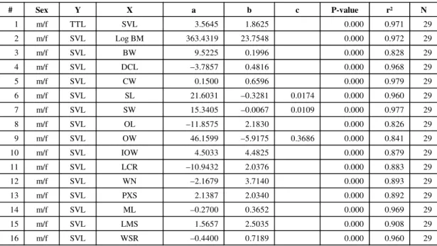
Table 2 and Fig. 2 show the regression equations and respective plots between body- and head-size variables and the snout-vent length (SVL) in wild individuals. Table 3 and Fig. 3 show the regression equations and respective plots between ratio variables and SVL in wild individuals. Due to the relatively small sample size, wild males and females are presented together. Table 4 and Fig. 4 show the regression equations and respective plots between body- and head-size variables and the snout-vent length (SVL) in captive animals. Table 5 and Fig. 5 show the regression equations and respective plots between ratio variables and SVL in captive animals.
# Sex Y X a b c P-value r² N
1 m/f TTL SVL 3.5645 1.8625 0.000 0.971 29 2 m/f SVL Log BM 363.4319 23.7548 0.000 0.972 29 3 m/f SVL BW 9.5225 0.1996 0.000 0.828 29 4 m/f SVL DCL –3.7857 0.4816 0.000 0.968 29 5 m/f SVL CW 0.1500 0.6596 0.000 0.979 29 6 m/f SVL SL 21.6031 –0.3281 0.0174 0.000 0.960 29 7 m/f SVL SW 15.3405 –0.0067 0.0109 0.000 0.977 29 8 m/f SVL OL –11.8575 2.1830 0.000 0.826 29 9 m/f SVL OW 46.1599 –5.9175 0.3686 0.000 0.841 29 10 m/f SVL IOW 4.5033 4.4825 0.000 0.879 29 11 m/f SVL LCR –10.9432 2.0376 0.000 0.883 29 12 m/f SVL WN –2.1679 3.7140 0.000 0.893 29 13 m/f SVL PXS 2.1387 2.0340 0.000 0.892 29 14 m/f SVL ML –0.2700 0.3652 0.000 0.969 29 15 m/f SVL LMS 1.5657 2.5035 0.000 0.908 29 16 m/f SVL WSR –0.4400 0.7189 0.000 0.960 29 Y = a + bX + cX² + dX³.
Sex: m/f = males and females. N: Sample size.
Minitab procedure: Stat → Regression → Fitted Line Plot (Polynomial Regression).
With the exception of BM, variables were not transformed because their orders of magnitude are similar and transformation did not improve results.
Quadratic element (c) was included in the equation (c ≠ 0) whenever significant (P-value ≤ 0.05). TABLE 2
With the exception of body mass (BM), log-transformation did not improve regression equa-tions for either wild or captive animals. Logarithmic transformation is a simple device that may ease and improve diagrammatic and statistical des-criptions of the effect of body size on other attri-butes (Peters, 1983). Regression equations for captive animals presented a higher coefficient of determination (r²) than the ones for wild animals. Body- and head-size variables presented a signi-ficantly higher r² than ratio variables for both wild and captive animals. They varied from 0.826 (OL) to 0.979 (CW) for body- and head-size variables (Table 2), and from 0.002 (RLSS) to 0.581 (RLST) for ratio variables (Table 3) for wild animals. For captive animals, in their turn, they varied from 0.916 (OW) to 0.993 (SW) for body- and head-size variables (Table 4), and from 0.003 (RLSS) to 0.934 (RLST) for ratio variables. The range of SVL relative to each equation can be found on the plots of Figs. 2 to 5.
The coefficients of determination of wild and captive animals concerning body- and head-size variables can be considered extremely high. Their main biological meaning is the apparent lack of
morphological variation on the patterns studied, which could be expected for captive but not for wild animals. They also mean that most of the head-size variables studied can be useful for predicting body length. This can be particularly interesting for the study of museum collections, or even poa-ching wastes, in which only crania are usually preserved or found relatively intact. However, the present study lacks adult wild individuals.
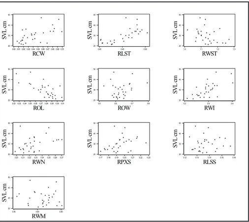
Some precaution is advised when using ratio variables for predicting body length. Some of these regression equations are not statistically significant (P-value > 0.100). This is the case for the following variables: ROW, RLSS, and RWM for wild, and ROW and RLSS for captive animals). Plots in Figs. 3 and 3 help to visualize these patterns.
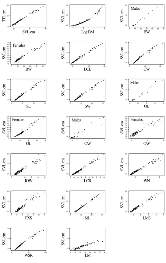
Besides helping to estimate body-size from head dimensions, the regression equations of the present study stress skull shape changes during the ontogenetic process. Non-linear equations express changes on the proportions of the skull, “accelerated” or “decelerated” on the inflexion points. For instance, the cranium of captive animals becomes relatively narrower as body size increases (see plot of CW in Fig. 4).
# Sex Y X a b c d P-value r² N
1 m/f SVL RCW –66.8226 150.884 0.000 0.370 29 2 m/f SVL RLST 7806.83 –52284.4 116487.0 –86021.1 0.000 0.581 29 3 m/f SVL RWST 79.0565 –43.1568 0.045 0.140 29 4 m/f SVL ROL 96.0670 –238.949 0.000 0.523 29 5 m/f SVL ROW 14.5130 24.6588 0.323 0.036 29 6 m/f SVL RWI –0.2700 103.195 0.000 0.437 29 7 m/f SVL RWN –2.5876 144.094 0.029 0.164 29 8 m/f SVL RPXS –6.9892 190.882 0.050 0.135 29 9 m/f SVL RLSS 24.8324 38.6619 0.805 0.002 29 10 m/f SVL RWM 41.2090 –21.6420 0.687 0.006 29 Y = a + bX + cX² + dX³.
Sex: m/f = males and females. N: Sample size.
Minitab procedure: Stat → Regression → Fitted Line Plot (Polynomial Regression).
With the exception of BM, variables were not transformed because their orders of magnitude are similar and transformation did not improve results.
Cubic element (d) was included in the equation (d ≠ 0) whenever significant (P-value ≤ 0.05).
Quadratic element (c) was included in the equation (c ≠ 0) whenever either quadratic or cubic element were significant (P-value ≤ 0.05).
TABLE 3
A similar and expected pattern can be seen on the mandible (see plot of WSR in the same figure). In both cases, regression equations are quadratic with the coefficient of the quadratic element being negative (see Table 4).
A somewhat sigmoid shape can be perceived on the relative growth curve of the eye-orbit length (OL) and width (OW) in captive animals. A po-sitive quadratic and a negative cubic element in the allometric equations of both cases show a period of fast relative growth in young followed by a period of slow relative growth of these regions
in adult animals. The smaller coefficient of the linear element of the OW equation than of the OL equation express the ontogenetic process of “elon-gation” suffered by the eye-orbits during initial development of the animals.
AGEAND SEXAS COVARIATESOF BODY SIZE
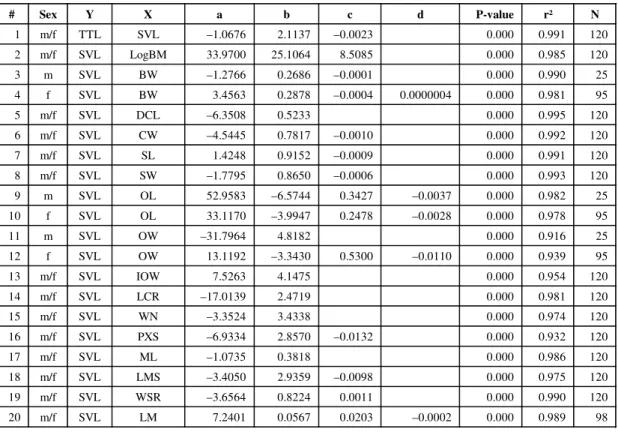
Table 6 shows the analysis of covariance (ANCOVA) of sex and age of captive animals in relation to the regression equations between morphometric variables and snout-vent length (SVL).
# Sex Y X a b c d P-value r² N
1 m/f TTL SVL –1.0676 2.1137 –0.0023 0.000 0.991 120 2 m/f SVL LogBM 33.9700 25.1064 8.5085 0.000 0.985 120 3 m SVL BW –1.2766 0.2686 –0.0001 0.000 0.990 25 4 f SVL BW 3.4563 0.2878 –0.0004 0.0000004 0.000 0.981 95 5 m/f SVL DCL –6.3508 0.5233 0.000 0.995 120 6 m/f SVL CW –4.5445 0.7817 –0.0010 0.000 0.992 120 7 m/f SVL SL 1.4248 0.9152 –0.0009 0.000 0.991 120 8 m/f SVL SW –1.7795 0.8650 –0.0006 0.000 0.993 120 9 m SVL OL 52.9583 –6.5744 0.3427 –0.0037 0.000 0.982 25 10 f SVL OL 33.1170 –3.9947 0.2478 –0.0028 0.000 0.978 95 11 m SVL OW –31.7964 4.8182 0.000 0.916 25 12 f SVL OW 13.1192 –3.3430 0.5300 –0.0110 0.000 0.939 95 13 m/f SVL IOW 7.5263 4.1475 0.000 0.954 120 14 m/f SVL LCR –17.0139 2.4719 0.000 0.981 120 15 m/f SVL WN –3.3524 3.4338 0.000 0.974 120 16 m/f SVL PXS –6.9334 2.8570 –0.0132 0.000 0.932 120 17 m/f SVL ML –1.0735 0.3818 0.000 0.986 120 18 m/f SVL LMS –3.4050 2.9359 –0.0098 0.000 0.975 120 19 m/f SVL WSR –3.6564 0.8224 0.0011 0.000 0.990 120 20 m/f SVL LM 7.2401 0.0567 0.0203 –0.0002 0.000 0.989 98 Y = a + bX + cX² + dX³.
Sex: m = males; f = females; m/f = males and females. N: Sample size.
Minitab procedure: Stat → Regression → Fitted Line Plot (Polynomial Regression).
With the exception of BM, variables were not transformed because their orders of magnitude are similar and transformation did not improve results.
Cubic element (d) was included in the equation (d ≠ 0) whenever significant (P-value ≤ 0.05).
Quadratic element (c) was included in the equation (c ≠ 0) whenever either quadratic or cubic element were significant (P-value ≤ 0.05).
Males and females presented separately when ANCOVA for sex was significant (P-value ≤ 0.05). See Table 6 for P-values. TABLE 4
Fig. 2 — Plots between body- and head-size variables for wild individuals (Log BM: log-transformed BM; SVL and TTL in cm, the others in mm). See Table 2 for regression equations.
ANCOVA may be used to compare males and females’ equations. It may also be useful to separate age from body-size effect on the regressions analyzed.
All body- and head-size variables, and all but three ratio variables (RWI, RWN, and RPXS) are significantly affected by body size (P-value > 0.100), or in other words, they can be considered size-dependent. One body-size (BW), six head-size (CW, SL, OL, OW, PXS, and WSR), and one ratio variable (ROL) are significantly affected by age (P-value > 0.100), i.e., they can be considered age-dependent.
At last one body-size (BW), two head-size (OL and OW), and five ratio variables (RCW, RLST, ROL, ROW, and RWN) are significantly affected by gender (P-value > 0.100).
Webb & Messel (1978) report a perceptible
sexual dimorphism in Crocodylus porosus
invol-ving interorbital width, which is not perceived in the present study. Hall & Portier (1994) found sexual dimorphism for 21 of 34 skull attributes, including DCL, ML, PXS, CW, OW, IOW, WCR, WN, and WSR. However, their results are possibly optmistic because they could not include age as a covariate of body size in their study of allometric
growth of Crocodylus novaeguineae. Some
varia-tion actually caused by age (independent of size) may be erroneously accounted as a difference between sexes, or sexual dimorphism.
The fact that all age-dependent variables are also size-dependent explains why it is so difficult to predict age of crocodilians based on single variable growth curves (see Verdade, 1997, for discussion).
# Sex Y X a b c d P-value r² N
1 m SVL RCW –214.951 367.644 0.000 0.901 25 2 f SVL RCW 8813.67 –36715.4 50550.9 –22872 0.000 0.839 95 3 m SVL RLST 219.636 –1106.28 1501.35 0.000 0.934 25 4 f SVL RLST 1706.86 –10271.9 20270 –12759 0.000 0.871 95 5 m/f SVL RWST –4630.87 13093 –11943.9 3557.43 0.000 0.452 120 6 m SVL ROL 541.144 –3188.86 4835.37 0.000 0.925 25 7 f SVL ROL –569.433 9513.45 –43137.6 60117.3 0.000 0.859 95
8 m SVL ROW 126.165 –123.61 0.034 0.180 25 9 f SVL ROW 26.2212 24.0213 0.534 0.040 95 10 m/f SVL RWI 104.269 –889.836 2910.8 –2443.13 0.000 0.808 120
11 m SVL RWN –109.85 549.146 0.000 0.674 25 12 f SVL RWN 575.858 –5780.9 19176.8 19294 0.000 0.810 95
13 m/f SVL RPXS 239.553 –2197.54 5885.48 0.000 0.118 120
14 m/f SVL RLSS 24.3543 108.483 0.565 0.003 120 15 m/f SVL RWM 404.504 –1595.72 1691.74 0.000 0.264 120
16 m/f SVL RLLMR 56.6448 –54.4797 0.068 0.835 98 Y = a + bX + cX² + dX³.
Sex: m = males; f = females; m/f = males and females. N: Sample size.
Minitab procedure: Stat → Regression → Fitted Line Plot (Polynomial Regression).
With the exception of BM, variables were not log-transformed because their orders of magnitude are similar and log-transformation did not improve results.
Cubic element (d) was included in the equation (d ≠ 0) whenever significant (P-value ≤ 0.05).
Quadratic element (c) was included in the equation (c ≠ 0) whenever either quadratic or cubic element were significant (P-value ≤ 0.05).
Males and females presented separately when ANCOVA for sex was significant (P-value ≤ 0.05). See Table 6 for P-values. TABLE 5
Fig. 3 — Plots between body-size and ratio variables for wild individuals. See Table 3 for regression equations.
Variable SVL Age Sex Variable SVL Age Sex
BM 0.000 0.812 0.308 RCW 0.003 0.392 0.026
BW 0.000 0.061 0.010 RLST 0.000 0.474 0.018
DCL 0.000 0.233 0.283 RWST 0.088 0.805 0.312
CW 0.000 0.012 0.192 ROL 0.002 0.033 0.007
SL 0.000 0.057 0.167 ROW 0.007 0.203 0.000
SW 0.000 0.480 0.989 RWI 0.292 0.509 0.376
OL 0.000 0.004 0.001 RWN 0.298 0.946 0.060
OW 0.000 0.032 0.004 RPXS 0.632 0.574 0.227
IOW 0.002 0.123 0.548 RLSS 0.058 0.327 0.746
LCR 0.000 0.308 0.347 RWM 0.002 0.367 0.582
WN 0.000 0.841 0.459 RLLMR 0.001 0.667 0.779
PXS 0.005 0.075 0.396
ML 0.000 0.128 0.173
LMS 0.000 0.521 0.830
WSR 0.000 0.020 0.448
LM 0.000 0.972 0.972
Minitab procedure: Stat → ANOVA → General Linear Model. Response (dependent variables): morphometric variables. Model (independent variable): SVL.
Covariates: Age and Sex.
TABLE 6
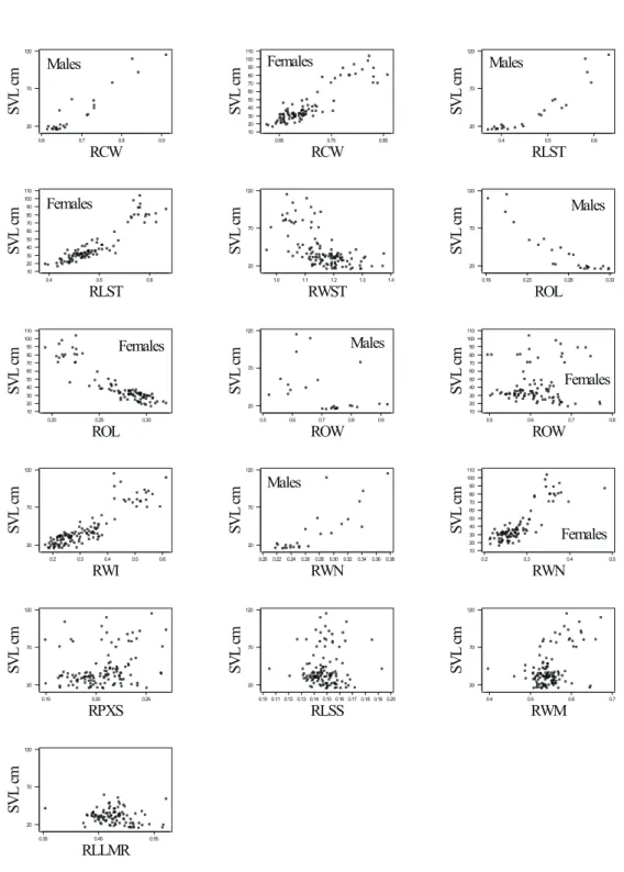
Fig. 4 — Plots between body- and head-size variables for captive individuals. Males and females presented together un-less stated otherwise. See Table 4 for regression equations. See Table 6 for ANCOVA P-values.
0.6 0.7 0.8 0.9 20 70 120 RCW SV L cm Males 0.85 0.75 0.65 110 100 90 80 70 60 50 40 30 20 10 RCW SV L cm Females 0.6 0.5 0.4 120 70 20 RLST SV L cm Males 0.6 0.5 0.4 110 100 90 80 70 60 50 40 30 20 10 RLST SV L cm Females 1.4 1.3 1.2 1.1 1.0 120 70 20 RWST SV L cm 0.33 0.28 0.23 0.18 120 70 20 ROL SV L cm Males 0.30 0.25 0.20 110 100 90 80 70 60 50 40 30 20 10 ROL SV L cm Females 0.9 0.8 0.7 0.6 0.5 120 70 20 ROW SV L cm Males 0.8 0.7 0.6 0.5 110 100 90 80 70 60 50 40 30 20 10 ROW SV L cm Females 0.6 0.5 0.4 0.3 0.2 120 70 20 RWI SV L cm 0.38 0.36 0.34 0.32 0.30 0.28 0.26 0.24 0.22 0.20 120 70 20 RWN SV L cm Males 0.5 0.4 0.3 0.2 110 100 90 80 70 60 50 40 30 20 10 RWN SV L cm Females 0.25 0.20 0.15 120 70 20 RPXS SV L cm 0.20 0.19 0.18 0.17 0.16 0.15 0.14 0.13 0.12 0.11 0.10 120 70 20 RLSS SV L cm 0.7 0.6 0.5 0.4 120 70 20 RWM SV L cm 0.55 0.45 0.35 120 70 20 RLLMR SV L cm
All of the sex-dependent variables are also size dependent, with the exception of RWN. However, its efficiency in predicting individual sex through discriminant analysis is low. Four sex-dependent variables (BW, OL, OW, and ROL) are also age-dependent, but the remaining four, all of them ratio variables (RCW, RLST, ROW, and RWN), are not. Age-dependent as well as sex-dependent variables are primarily located on the cranium. Only one age-dependent (WSR) and sex-independent variable is located on the mandible. Sexual dimorphism was detected in the allometric growth of BW, OL, OW, RCW, RLST, ROL, ROW, and RWN. With the exception of BW, all of these morphometric variables are located in the cranium and none in the mandible. This may be evolutionarily related to the visual recognition of gender when individuals exhibit only the top of their heads above the surface of the water, a usual behavior of crocodilians. A multivariate approach for the study of sexual dimorphism is discussed by Verdade (1997).
Acknowledgments — This study is a part of the dissertation presented to the Graduate School of the University of Flo-rida in partial fulfillment of the requirements for the degree of Doctor of Philosophy. This program was supported by the Conselho Nacional de Desenvolvimento Científico e Tecnológico – CNPq (Process N. 200153/93-5) and the University of São Paulo, Brazil. I am thankful to Prof. F. Wayne King, J. Perran Ross, Lou Guillette, Richard Bodmer, Mel Sunquist, George Tanner, Phil Hall, and Irineu U. Packer for their ideas and comments on the manuscript. Edson Davanzo, Fabianna Sarkis, and Rodrigo Zucolotto helped to measure the animals. Data set is available with the author.
REFERENCES
ALLSTEAD, J. & LANG, J. W., 1995, Sexual dimorphism in the genital morphology of young American alligators,
Alligator mississippiensis. Herpetologica,51(3): 314-25. BOOKSTEIN, F. L., 1989, “Size and shape”: a comment on
semantics. Systematic Zoology,38(2): 173-80. CHABRECK, R., 1963, Methods of capturing, marking and
sexing alligators. Proc. Ann. Conf. Southeastern Assoc. Game Fish Comm., 17: 47-50.
CHABRECK, R. H., 1966, Methods of determining the size and composition of alligator populations in Louisiana. Proc. Ann. Conf. SE Assoc. Game Fish Comm., 20: 105-12. CHOQUENOT, D. P. & WEBB, G. J. W., 1987, A
photo-graphic technique for estimating the size of crocodilians seen in spotlight surveys and quantifying observer bias in estimating sizes. pp. 217-224. In: G. J. W. Webb, S. C. Manolis & P. J. Whitehead (eds.), Wildlife Manage-ment: Crocodiles and Alligators. Surrey Beatty & Sons Pty Lim., Chipping Norton, Australia.
GOULD, S. J., 1966, Allometry and size in ontogeny and phylogeny. Biol. Rev., 41: 587-640.
HALL, P. M. & PORTIER, K. M., 1994, Cranial morphom-etry of New Guinea crocodiles (Crocodylus novae-guineae): ontogenetic variation in relative growth of the skull and an assessment of its utility as a predictor of the sex and size of individuals. Herpetological Monographs, 8: 203-225.
HUTTON, J. M., LOVERIDGE, J. P. & BLAKE, D. K., 1987, Capture methods for the Nile crocodile in Zimbabwe. pp. 243-247. In: G. J. W. Webb, S. C. Manolis & P. J. White-head (eds.), Wildlife Management: Crocodiles and Alli-gators. Surrey Beatty & Sons Pty Lim., Chipping Norton, Australia.
IORDANSKY, N. N., 1973, The skull of the Crocodilia. pp. 201-262. In: C. Gans & T. S. Parsons (eds.), Biology of the Reptilia. Vol. 4. Morphology D. Academic Press, London.
MAGNUSSON, W. E., 1983, Size estimates of crocodilians.
Journal of Herpetology,17(1): 86-88.
MINITAB, 1996, Minitab for Windows Release 11. Minitab, Inc., State College, PA, USA.
PETERS, R. H., 1983, The Ecological Implications of Body Size. Cambridge University Press, Cambridge. SCHMIDT-NIELSEN, K., 1984, Scaling: Why is Animal Size
so Important? Cambridge University Press, Cambridge. SOKAL, R. R. & ROHLF, F. J., 1995, Biometry: the Prin-ciples and Practice of Statistics in Biological Research. W. H. Freeman and Company, New York.
VERDADE, L. M., 1997, Morphometric Analysis of the Broad-snouted Caiman (Caiman latirostris): An Assess-ment of Individual’s Clutch, Body Size, Sex, Age, and Area of Origin. Ph.D Dissertation. University of Florida, Gainesville, Florida, USA, 174p.
VERDADE, L. M. & KASSOUF-PERINA, S. (Eds.), 1993,
Studbook Regional do Jacaré-de-papo-amarelo (Caiman latirostris): 1992 / 1993. Sociedade de Zoológicos do Brasil. Sorocaba, São Paulo, Brasil.
VERDADE, L. M. & MOLINA, F. B. (eds.), 1993, Studbook Regional do Jacaré-de-papo-amarelo (Caiman latiros-tris): Junho 1991-Junho 1992. ESALQ, Piracicaba, São Paulo, Brasil.
VERDADE, L. M. & SANTIAGO, M. E. (eds.), 1991, Stud-book Regional do Jacaré-de-papo-amarelo (Caiman lati-rostris). CIZBAS/ESALQ/USP. Piracicaba, São Paulo, Brasil.
VERDADE, L. M. & SARKIS, F., In press, Studbook Re-gional do Jacaré-de-papo-amarelo (Caiman latirostris):
1993/1997. ESALQ, Piracicaba, São Paulo, Brasil. WALSH, B., 1987, Crocodile capture methods used in the
Northern Territory of Australia. pp. 249-252. In: G. J. W. Webb, S. C. Manolis & P. J. Whitehead (eds.), Wildlife Management: Crocodiles and Alligators. Surrey Beatty & Sons Pty Lim., Chipping Norton, Australia. WEBB, G. J. W. & MESSEL, H., 1977, Crocodile capture
WEBB, G. J. W. & MESSEL, H., 1978, Morphometric analy-sis of Crocodylus porosus from the north coast of Arnhem Land, northern Australia. Australian Journal of Zoology 26: 1-27.