Microeconomics of Space – a Selective Survey

Carlos Pestana Barros & Nicolas Peypoch

A Comparative Analysis of Productivity Change in Italian and

Portuguese Airports

WP 006/2007/DE

_________________________________________________________

José Pedro Pontes

Microeconomics of Space – a Selective Survey

WP 03/2011/DE/UECE

_________________________________________________________

Department of Economics

W

ORKING

P

APERS

ISSN Nº 0874-4548

School of Economics and Management

Microeconomics of Space – a Selective Survey

by

José Pedro Pontes1

1.

Introduction: why to study the microeconomics of space?

A representative firm takes two kinds of decisions concerning space: its

location and the set of prices it quotes in each point in space.2 Why is it important for

an applied micro economist to examine these decisions?

Let us begin by defining the terminology. By “fob price” we mean the price

set by the firm in its location, while “delivered price” labels the full price that the

consumer pays at its living place, including the transport cost of the product between

the locations of supply and demand.

Microeconomics has been traditionally dominated by the paradigms of

“perfect market” and “perfect competition”. A “perfect market” is a structure

supporting transactions such that each consumer and each producer know the prices

bid by all consumers and the prices asked by all producers. “Perfect competition”

means that, among other assumptions, the products supplied by the firms are

completely homogeneous, so that each consumer is indifferent among them when they

are supplied at the same price. Moreover, “perfect competition” means that the

number of producers competing in each market is high. Together, these two

1 _{ISEG, Technical University of Lisbon and UECE. Contact address: [email protected].}

The author acknowledges financial support from Fundação para a Ciência e a Tecnologia through Pluri-annual fincncing program of UECE.

2

A third type of spatial decision which will not be tackled here concerns the amount of land

assumptions (homogeneity and large number of producers) ensure that each firm is

arbitrarily small in relation to the market, so that it cannot influence the price and that

it faces an infinitely elastic demand curve.

“Perfect market” and “perfect competition” jointly determine that each

product has a unique price at the market where the product is traded. For both

conditions to hold, the market should be close to a “point” in geographical terms. The

word “market” originally meant this physical “meeting point” (for instance, the stock

exchange, or the commodities exchanges).

However, economic agents are spread over space rather than clustered in

market “points”. The model by ENKE (1942) tries to reconcile the dispersed pattern

of agents with the assumptions of perfect competition (see Figure 1).

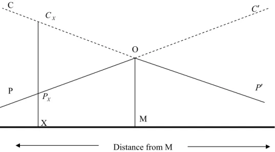
In Figure 1, the consumers and producers are uniformly distributed along the

line. All transactions are made at a “central exchange” in M, where a market price

OM is formed through the meeting of all sellers and buyers. However, the real prices

which are received by the producers (given by the curvePOP′) and paid by the

consumers (given by the curveCOC′) differ from the market prices on account of X

X

Distance from M X

Figure 1: ENKE (1942)’s model of “central exchange”

P′

C′

X

X

P

X

X

C

C

M O

freight charges. The slopes of line segments CO, PO and OC′ ,OP′ reflect the

transport cost by unit of distance. Hence, a consumer located in X pays a delivered

price C and a producer in the same location receives a fob price_X P . The difference _X

between these prices and the market price corresponds to the transport cost between

the “central exchange” M, the locations of the consumer and of the producer in X.

Why do the seller and the buyer placed in point X use the central exchange in

M in order to transact instead of trading locally? After all, exchanging the product

locally in X would allow saving transport costs for both groups of agents. Instead,

locating the transactions in M brings two kinds of advantages:

1. In M, a large number of homogeneous buyers

and sellers meet, so that none enjoys market power: each firm faces an infinitely

elastic demand function, so that “perfect competition” prevails.

2. The localization of transactions yields “perfect

information” of each side of the market about the prices bid and asked. Each agent has

this kind of information without having to incur search costs: he must not travel

between the sellers in order to inquire about prices.

However, the size of the region should be bounded from above. A too large

region entails very high transport costs that do not allow the use of the “central

exchange” as a transaction device.

Hence, it is usually assumed that the consumers and producers in an area are

partitioned in a set of “regions” (PONTES, 1987). This partition is independent of the

regional prices of the product. Within each “region”, fixed numbers of consumers and

producers transact through a “central exchange”. Trade between “regions” takes

place through the network of “central exchanges”.

Demand by the consumers and supply by the producers are modeled by

means of regional functions of demand and supply. Besides consumers and producers,

a third category of agents (labeled as “traders”) transports the product between

regions. Let the term “excess supply” mean the difference between regional supply

and regional demand at a given price. The equilibrium is a profile of regional prices

1. The aggregate (across all regions) excess supply

is zero, i.e. total exports equal total imports of the product in the

spatial economy.

2. Each delivered price should not exceed the sum

of the fob price and the transport cost between the origin and

destination regions (i.e., the profit of the trader is non-positive).

3. If the export flow from an origin region to a

destination is positive, then the delivered price equals the sum of the

fob price and the transport cost between the regions (i.e., the profit of

trader is zero).

4. If the delivered price is smaller than the sum of

the fob price and the transport cost (i.e., the trader’s profit is

negative), the export flow is zero.

These conditions amount to the traditional conditions for a set of prices to be

a competitive equilibrium, namely:

• Individual equilibrium: at these prices every agent maximizes either utility (consumers through the regional

demand functions) or profit (producers through the regional supply

functions; traders through the equilibrium conditions 2, 3 and 4).

• Market equilibrium: at these prices, total exports equal total imports, so that the interregional market of the

product clears (equilibrium condition 1).

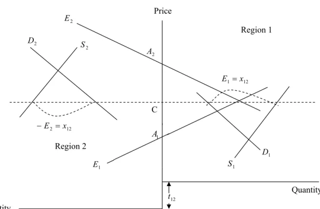
Where: 1,2 regions in functions Demand , ₂

1 D ≡ D 1,2 regions in functions Supply , ₂

1 S ≡ S 1,2 regions in functions supply Excess , ₂

1 E ≡ E 2 1, regions in autarky in prices m Equilibriu , ₂

1 A ≡ A trade nal interregio under price m equilibriu fob ≡ C regions two e between th cost Transport 12 ≡ t trade nal interregio under price Delivered 12 ≡ +t C 2 region to 1 region from Exports 12 ≡ x 1 D

With more than three regions it becomes difficult to find an analytical

solution to the spatial price equilibrium model. This solution becomes feasible if we

state the model as an optimization problem where either aggregate transport cost is

minimized or social welfare is maximized subject to the following constraints (see

PONTES, 1987):

1. Interregional product flows are nonnegative.

2. Aggregate imports of the product by a region

should not be lower than regional demand.

3. Aggregate exports by a region should not

exceed regional production.

Then, it is easy that the necessary conditions of these problems reproduce

the conditions of the spatial equilibrium problems: Kuhn-Tucker multipliers define

regional prices that clear supply and demand in each region; at these prices, all

categories of agents (consumers, producers and “traders”) maximize either utility or

profits.

However, the spatial equilibrium model bears a contradiction that follows

from the fact that the partition of consumers and producers across the regions is fixed.

Nevertheless, it determines the formation of equilibrium prices. Or it is widely known

that the matching between producers and consumers is influenced by regional prices.

If p₁ is much higher thanp₂, then consumers in region 1 will prefer to buy the

product in region 2, and this specially if t₁₂is not too high. In sum, we have the

In order to avoid this indetermination, the trading units should be conceived

as individual consumers and producers rather than “regions” or “central exchanges”.

However this shift would undermine the assumptions of “perfect competition” (large

number of homogeneous sellers in each point of space) and “perfect market” (zero

search costs of information about asked and bid prices). The consideration of space

makes perfect competition an unrealistic description of the operation of markets.

Another instance of breakdown of the competitive price system can be found

in KOOPMANS and BECKMANN (1957) following from the combination of the

indivisibility of the productive activity and the technological interdependence of the

location of plants through the exchange of intermediate goods.

It is an empirical fact that productive plants are often indivisible. For many

productive activities, there is a minimum efficient scale of production. Let us assume

that there are nindivisible plants that must be located or assigned to n different Regional prices

Regional functions of

supply and demand

Distribution of consumers and

locations. There are _n2

assignments which are each given by a pair plant-location. For each of these assignments a profit score is defined. We make now the crucial

assumption that the plants are technologically independent, i.e. the profitability of a

plant in a location does not vary with the location chosen by another plant.

For instance, if there are 4 plants and 4 locations, a possible set of profit

scores is given by the matrix:

Plants

Locations

1 2 3 4

1 25 20 5 19 2 18 3 0 12 3 22 4 2 12 4 16 7 -2 10

Then, to find feasible locations for the plants amounts to selecting a unique

plant –location pair in each row and column of the matrix. If we compare all the

feasible assignments from the viewpoint of aggregate profitability, we obtain the

optimal location pattern. In this example, the optimal assignment is given by

Locations

Plants

1 2 3 4

1 25 20 5 19

2 18 3 0 12

3 22 4 2 12

4 16 7 -2 10

In this table, the underlined cells express optimal locations. The overall

profitability of the optimal assignment is 52 units. It should be remarked that the most

Plant

s

Each feasible assignment can be expressed by a permutation matrix, i.e. a

matrix that has exactly a 1 in each column and row and zeros elsewhere. The

permutation matrix of the optimal assignment is

T

h

i

s

is a problem of centralized planning. Can the optimal allocation be sustained if instead

the owners of plants take decentralized location decisions based on their knowledge of

profit scores and on some kind of prices (namely rentals of the plants and sites)?

The answer is yes. This can be seen if we introduce the possibility of

fractional assignments where a plant can be distributed by several locations and a

location can be occupied by shares of different plants. We require that the sum of

plant shares across locations and across plants sums 1 so that a location is occupied

exactly by a plant. Then, the assignment that maximizes overall profit can be found by

means of a linear programming problem.

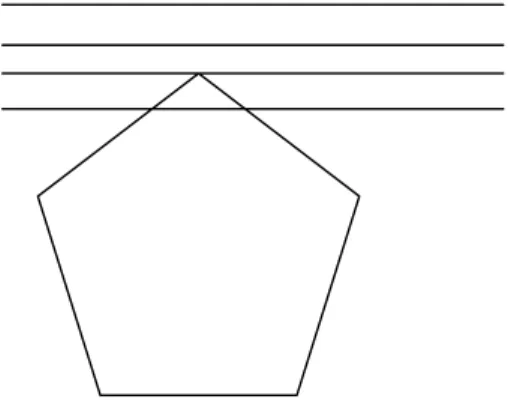
The feasible set of a linear programming problem is a convex set with a finite

number of extreme points (vertices). In such a problem, the optimum is reached either

in a vertex or in two adjacent vertices. In the latter case, it is also reached in the face

that connects the two adjacent extreme points (see Figure 3). Locations

1 2 3 4

It can be established that the extreme points of the feasible set of the linear

programming problem correspond to the permutation matrices in the problem of

integral optimal assignment. Hence, when we exclude fractional assignments and pass

to the optimal location of indivisible plants, we do not lose any optimal solutions.

Since a feasible solution of a linear programming location problem is optimal

if and only if it has associated a set of prices (rentals of locations and of plants in this

case), the same property holds for the optimal locations of indivisible plants.

Let us assume that there is a rental of each location and a rental of each plant

and a score of profitability for the assignment of the plant to the location. Then, the

sum of the costs (the rentals of location and plant) is higher than or equal to the profit

of the assignment. Only in the case of an optimal plant /location assignment is the

relation satisfied as equality. This means that, given the plant rentals, the owner of a

location maximizes its rental in the optimal assignment. Conversely, given the

location rentals, the owner of a plant maximizes its rental also in the optimal

assignment. The set of prices (rentals) together with the knowledge of the profits

related with each location-plant pair sustains the optimal set of locations of indivisible

plants are indivisible (may be, on account of increasing returns to scale in

production).

Let us assume now instead that plants are technologically interdependent

through the exchange of intermediate goods. Now the profit of a plant depends not

only upon its location but also on the locations of the plants that supply its

intermediate goods. The objective function of the integral assignment problem

contains, besides the term connected with the pairing of plants and locations, a term

that represents the transport cost of the traded inputs

Again, we can pass to a fractional assignment problem, where each plant is

distributed across all locations and each location can be occupied by shares of all

plants. This problem assumes that plants are divisible and it has the same constraints

as before (namely the shares of a plant should sum 1 across locations and the shares of

plants in a given location should sum 1 too). An additional constraint arises: the sum

of the production of each intermediate good in a location with the imports of this good

into that region should equal the use of the good in the region plus the amount of it

that is exported.

It is clear that no integral solution with indivisible plants is an optimum of

the fractional assignment problem. Assume that the gross profit score of each plant is

invariant with relation to location. Then it is clear that profit maximization across

locations by each plant is equivalent to minimization of the costs related with the

movement of intermediate goods among plants. Consequently, if there are n plants

and n locations, the optimum of the fractional assignment problem occurs when

n

1 of

each plant is placed in each location because then the transport costs of the

intermediate goods are zero.

As no integral assignment is an optimum of linear programming (fractional

assignment) problem, there is no competitive price system that sustains the optimal

plants and sites. Given any prices, there will always be a plant owner that has an

incentive to shift location. As KOOPMANS and BECKMANN say:

There will be always be an incentive for someone to

seek a location other than the one he holds… there would be a

continual game of musical chairs. (KOOPMANS and

BECKMANN, 1957, p- 70)

2.

Location of firms under oligopoly

.

The same conclusion (that a perfectly competitive outcome is incompatible

with the existence of a lengthy spatial market) can be reached from the viewpoint of

oligopoly, i.e. an industry with few sellers. COURNOT (1838) devised the following

framework. Two identically located firms (for instance, two springs of mineral water)

sell homogeneous products to consumers agglomerated in a market that is a “point” (a

market without length). Each firm competes through the choice of an output and faces

the following trade-off: by selling one more unit it receives an additional price while

depressing the prices at which all the other units are sold. Then a Cournot equilibrium

(later generalized as “Nash equilibrium”) is achieved when each firm sells a quantity

that maximizes its profit given the output chosen by its rival. In equilibrium, the

output chosen by each firm is a “best reply” to the competitor’s output, so that no firm

has an incentive to deviate unilaterally from the equilibrium output. When these

outputs are sold, the equilibrium price of the homogenous good (the mineral water) is

strictly higher than the unit cost of production, so that each firm makes a positive

profit.

BERTRAND (1883) criticized Cournot’s results, saying that firms really

compete through the quoting of prices rather than quantities. In this setting, two firms

producing an homogenous good under constant and equal marginal costs will charge

equilibrium prices equal to marginal costs. Consequently, both firms will have zero

profits and the result is similar to perfect competition.

The rationale behind Bertrand’s claim is the discontinuity of the demand

In this level, if a firm charges a price slightly lower than the competitor’s, it will get

all the consumers. Since this applies to both firms, prices will fall successively until

they reach the unit production costs. Demand discontinuity is crucially linked with the

homogeneity of the two products.

HOTELLING (1929) restores the noncompetitive outcome under price

competition by assuming that the market is lengthy (a line segment) rather than a

point. Figure 4 depicts the spatial market.

The consumers are uniformly spread in a line segment of length l (which

may represent Main Street). Two firms selling homogenous products are located in

points A and B. The distances between each firm and the closest extreme point of the

market are given by a and by b, respectively.

The firms have identical constant unit production costs, which we assume to

be zero w.l.g. The firms sell fob mill prices p₁and p₂and each consumer carries the

product in the distance between the firm’s location and his address, the transport cost

per unit of distance being given by t. The delivered price of the product for a given

consumer is the sum of the fob mill price and the transport cost. It is further assumed

that each consumer purchases a unit of the product per unit of time irrespective of its

price.

This model deals with two different problems: the setting of fob mill prices

and the choice of locations by the firms. He implicitly assumes that the firms firstly

select locations and then set prices. This is a two stage game that is, as usual solved B

A

b y

x a

by backward induction. Thus we first tackle the formation of prices and then the

firms’ locations.

The main point stressed by HOTELLING (1929) is that the demand

addressed to each firm becomes continuous if the firms agree somehow to share the

market, i. e. if the difference of the fob mill prices does not exceed the transport cost

in the distance between the firms:

(

)

1 2

p − p ≤t x+y

( )

1

If this condition is met, the consumers placed between the firms will be split

in two market areas whose boundary is given by the condition of indifference for the

marginal consumer to purchase the product to either firm. This means that the

delivered price of each firm to that consumer is the same. The market area of each

firm comprehends its hinterland (a or b) and the consumers in the intermediate region

for whom it is cheaper in terms of delivered price to purchase to the firm (segments x

or y). If a firm lowers its fob mill price, some consumers will be transferred from the

competitor to the firm. However, as long as the previous condition is met, the

competitor will retain a share of its customers, who prefer to buy from it at a

somehow higher price, so that the demand functions addressed to the firms are

continuous.

As the outputs of the firms are proportional to the size of market areas, it is

easy to write the profit functions of the firms and derive equilibrium fob mill prices:

the price set by each firm maximizes its profit given the price set by the rival firm.

Each price is a best reply to the price set by the rival firm. It is easy to show that these

prices are strictly above the unit production costs and firms have positive profits.

Consequently, the substitution of a lengthy market for a market with an exact point

leads the economy away from the perfectly competitive outcome of Bertrand and

This model gave birth to a huge strand of literature. A share of this literature

has devoted itself to generalize the assumptions of the model, but it is more

interesting to recall the papers that have addressed the consistency and validity of the

result.

D’ASPREMONT et AL. (1979) have shown that HOTELLING´s prices are

not (unlike Cournot prices) Nash equilibrium prices, since for each firm, its price is a

best reply only if it accepts to share the market with the competitor. The firms in

HOTELLING (1929) choose profit maximizing prices constrained to the price set

defined by condition (1). Were the prices of a Nash equilibrium type, they would have

to be profit maximizing in the whole price set

[

0,∞

)

and not only in the price set defined by inequality (1).

The proof by D’ASPREMONT et AL (1979) proceeds as follows. If there is

a Nash price equilibrium, then the prices

(

p₁,p₂

)

should belong to the price set

defined by condition (1), because otherwise one firm would have zero sales and profit

and it would have an incentive to change its price. However, if prices belong to this

set, they form a Nash equilibrium if and only if no firm has incentive to deviate to a

price outside the set in order to undercut the rival out of business. The authors prove

that this is the case if the firms locate far apart (with symmetric locations, outside the

quartiles), but not if they locate close. In the latter case, each firm can drive the

competitor out of business with a modest price cut and a price war follows.

Figures 5-a and 5-b illustrate the cases of existence and absence of a Nash

price equilibrium in HOTELLIG’s (1929) oligopoly. We represent the profit function

1 p

(

)

2

p +c x+y

(

x y

)

c

p₂ − +

(

1 2

)

1 p ,p

π

In Figure 5, it is plotted the profit of firm1 as a function of its mill price p₁,

given the price of its competitor p₂. The profit function exhibits three regions

separated by two discontinuities. If p₁< p₂−t x

(

+y

)

, firm 1 sells to all customers, so

that its profit is a linear function of the price. If p₂−t x

(

+y

)

< p₁< p₂+t x

(

+y

)

, they share the market and the profit function is quadratic in price. For

(

)

1 2

p > p +t x+y , demand addressed to firm 1 and profit are zero.

It follows from the previous discussion that a Nash equilibrium in prices

exists if and only if the profit of sharing the market with the rival firm exceeds the

profit of undercutting it, i.e. if the local maximum of the profit function in the

quadratic region exceeds the local maximum in the linear region. There is a Nash

(

1 2

)

1 p ,p

π

(

)

2

p −t x+y

1 p

Figure 5-b: Nonexistence of price equilibrium in HOTELLING’s oligopoly

(

)

2

equilibrium in Figure 5-a but not in Figure 5-b. Equilibrium occurs whenever the

firms are distant apart so that the cost of undercutting the rival is high for each firm.

However, this criticism seems unjustified since HOTELLING (1929) did not

claim that his prices were analogous to Cournot’s. Instead, he defended that his prices

are (locally) stable.

The concept of stability of a dynamic variable, whose law of motion is

described by a differential or difference equation, can be shortly described as follows.

Let the equilibrium be a stationary point: if the variable reaches that value, it stays

there indefinitely. This equilibrium is stable in a given set if, when it starts from any

value within that set, it converges to the equilibrium as time tends to infinity. The

degree of stability is measured by the size of the reference set. The variable is said to

be locally stable if it is stable in a small neighborhood around equilibrium.

HOTELLING (1929) argues that his prices have that property of (local)

stability. The possibility of undercutting by the firms is ruled out by some degree of

collusion. Each firm realizes that to launch a price war will be detrimental for both

firms and this will be avoided:

It is of course, possible that A feeling stronger than his

opponent and desiring to get rid of him once for all, may reduce his

price so far that B will give up the struggle and retire from business.

But during the continuance of this sort of price war A’s income will

be curtailed more than B’s. In any case its possibility does not affect

the argument that there is stability, since stability is by definition

merely the tendency to return after small displacements. A box

standing on end is in stable equilibrium, even though it can be tipped

over. (HOTELLING, 1929:50).

This author is aware that if the firms get close, the mass of intermediate

But the danger that the system will be overturned by the

elimination of one competitor is increased. The intermediate segment

of the market acts as a cushion as well as a bone of contention; when

it disappears we have Cournot’s case and Bertrands’s objection

applies. Or, returning to the analogy of the box in stable equilibrium

though standing on end, the approach of B to A corresponds to a

diminution in size of the end of the box. (HOTELLING, 1929:52)

In this case, equilibrium prices fit into the definition of “local Nash

equilibrium prices”: prices which are mutually best replies in a neighborhood of the

equilibrium. Small deviations from equilibrium are ruled out by considerations of

private profitability of the firm. Larger deviations entailing the undercutting of the

rival are excluded by the consideration that the rival will retaliate and launch a

mutually destructive price war.

HOTELLING (1929) contended that price equilibrium becomes “less stable”

when firms choose close locations. Instead D’ASPREMONT el AL (1979) sustained

that whenever firms get too close a Nash price equilibrium ceases to exist. These are

two different ways to express the same basic idea. However, these two ways lead to

different conclusions about the locations selected in equilibrium by the firms.

As we have said before, the economy is modeled by a game where firms

select locations firstly and then prices. Each firm anticipates the impact of its location

choice on the subsequent intensity of price competition. HOTELLING (1929)

concludes that each firm has an incentive to move towards the location of the

opponent in order to increase the mass of captive consumers in its hinterland.

Consequently, the equilibrium of locations will entail agglomeration with both firms

in the market center: it is the so called “Principle of Minimum Differentiation”. This

principle means that price competition is not strong enough to countervail the

advantages for the firms to locate in a central position in relation to the mass of

D’ASPREMONT et AL. (1979) have a different point of view. They

contend that the absence of a Nash price equilibrium when firms are close invalidates

the “Principle of Minimum Differentiation”. They rewrite the model using a quadratic

function tx2, where t is the transport cost parameter and x is distance. With this

function, they argue that there exists a Nash price equilibrium for any firms’

locations. Moreover, competition in the second stage will be strong enough to lead the

firms to relax price competition by locating in the extreme points of the market in the

context of a situation of maximal differentiation.

Our personal opinion is that HOTELLING’s result is more consistent than

those by their critics. Firstly, he did never contend that his prices are Nash equilibrium

prices. He rather said only that they are prices endowed with “local stability”.

Secondly, real transport cost functions usually exhibit economies of scale, i.e. they are

concave in distance rather than convex. From this it follows that agglomeration of

competitors is a much more empirically common result than dispersion so that in the

end HOTELLING (1929) was (approximately) right.

The fact that competition among firms does not countervail the advantages

for the firms to agglomerate near the central point of the market becomes more

evident if we consider that they compete in quantities rather than in prices (as in

ANDERSON and NEVEN, 1991).

Let us assume instead a spatial oligopoly with two different assumptions.

Firstly, firms A and B compete in each market point r selling quantities of

outputq1

( )

r andq2

( )

r . Secondly, they carry themselves the product between their

locations and the customers’. The behavior of the consumers in each market point r is

expressed by a linear inverse demand function. The game has two stages: firstly, the

firms choose locations; secondly, they select quantities of output in each market point.

The assumption on the transport cost function t

()

. is more general than in

HOTELLING (1929) and D’ASPREMONT et AL. (1979). It is assumed that t

()

. is:

• Increasing

• t

( )

0 =0

Then, it can be proved that, with convex transport costs and assuming that

each firm sells a positive output in each market point, there exists a unique

equilibrium for the location-quantity duopoly. In this equilibrium, both firms locate

in the market center.

The assumption on the convexity of the transport cost function is crucial. Let

us assume that a firm is located in 2

l

(the market center) and the other one is placed

between 2

l

and l. If it shifts to 2

l

, the second firm increases the profits that it makes

with the consumers to whom it gets closer (in the segment

[

0,x₂

]

) and decreases the profits with the consumers from whom it gets far away (in the segment

[

x2,l

]

). The

former line segment is larger than the latter, this being the first reason behind the

profitability of the move by the firm towards the center.

The second reason has to do with the convexity of the transport cost function.

With this kind of function, profits of the firm moving towards the center increase

faster in the segment

[

0,x₂

]

than they will decrease in the segment

[

x₂,l

]

, because marginal transport costs (per unit of distance) increase with distance. Consequently,

they increase more intensively in segment

[

0,x₂

]

than in

[

x₂,l

]

.

It can also be easily concluded that, with a concave transport cost function,

central agglomeration may not be an equilibrium set of locations.

Summing up, we can conclude that the centrifugal force of competition

among firms is not strong enough to compensate the drive by each firm toward the

market center in order to obtain accessibility to the whole set of consumers.

The location of oligopolistic firms has been renewed more recently by

BELLEFLAMME et AL (2000). In their model, the economic space is made by two

identical regions, A and B, each one endowed with the same number of consumers.

Thus, by contrast with the previous oligopoly model, there is no natural “central

We assume first that there are two firms selling differentiated products. Each

firm carries its product to the customers, so that it can price discriminate across

markets. We make the assumption of a quadratic utility function for the customers

given by:

(

) (

)

(

)

1 2 0

2 2 2 1 2 1 2

1,q q q ₂ q q qq q

q

U  + − +

     − +

=α β δ (2)

Where the output q_i

(

i=1,2

)

is the quantity consumed of differentiated product i _and q₀ is the quantity of an outside good. The following relations hold:

β δ

α>0and0≤ < . The maximization of this utility by the consumers subject to a

budget constraint determines that each firm faces a linear demand function defined on

the prices of both varieties:

(

j i

)

i

i a bp d p p

q = − + − (3)

where a≡α

(

β +δ

)

,b≡1

(

β +δ

)

and d ≡δ

[

(

β −δ

)(

β +δ

)

]

hold.

In (3), parameter d measures inversely the degree of differentiation of the

products. These will be independent if d=0. By contrast, they will be perfect substitutes when d→∞ holds.

In order to ship its product to another region each firm bears a unit transport

cost t. The production costs of the firms depend on their relative locations. If the

firms stay in different locations, each firm’s unit production cost is c>0. If they locate in the same region, there will be positive region-specific localization economies

that decrease their unit production costs. These become expressed as

K

c−θ

(

K= A,B

)

, the term θ_Kmeasuring the regional intensity of agglomeration economies. In what follows, it is assumed that θ_B ≤θ_A <c.

The concept of localization economies goes back to Alfred MARSHALL

(1949) and expresses the fact that the production costs are reduced when firms

belonging to the same industry locate in the same region. According to MARSHALL

(1949) these cost savings can be modeled as non-market interactions and be classified

1. Informal and unpredictable transfers of technological knowledge

among firms (spillovers), that stem from the mere closeness of their employees. These

kind of spillovers cannot be carried through electronic communication and they imply

face-to-face contact. As MARSHALL says:

The mysteries of the trade become no mysteries; but are as it were in the air, and children learn many of them unconsciously. Good work is rightly appreciated, invents and improvements in machinery, in processes and the general organization of business have their merits promptly discussed: if one man starts a new idea, it is taken up by others and combined with suggestions of their own; and thus it becomes the source of further new ideas. (MARSHALL, 1944: 225)

2. There is a difference between the skills that workers have and those

that are required by the firms, so that the problem of assigning each worker to each

firm in a “right” way is always present. If this matching is inefficient, each worker

has to support training costs in order to compensate the gap between its skill and the

one that is required by the firm. High training costs lead the workers to migrate to

other regions and the scarcity of labor tends to reduce the agglomeration of firms. As

MARSHALL says:

Again, in all but the earliest stages of economic development a localized industry gains a great advantage from the fact that it offers a constant market for skill. Employers are apt to resort to any place where they are likely to find a good choice of workers with the special skill they require; while men seeking employment naturally go to places where there are many who need such skill as theirs and where therefore it is likely to find a good market. The owner of an isolated factory, even if he has access to a plentiful supply is often put to great shifts for want of some special skilled labor; and a skilled workman, when thrown out of employment in it, has no easy refuge …These difficulties are still a great obstacle to the success of any business in which special skill is needed, but which is not in the neighborhood of others like it: they are however being diminished by the railway, the printing press and the telegraph. (MARSHALL, 1949: 225/6)

3. A final type of economies of localization follows from the exchange of

intermediate goods among firms. If several firms producing a consumption good

cluster in space, the workers in each firm are a source of demand for the other firms.

The resulting increase in market size allows a deepening of the division of labor, with

the separation between firms producing final goods and firms producing intermediate

levels. On the one hand, the production of each input can be geographically

concentrated in a single firm allowing the emergence of economies of scale. On the

other hand, each firm producing the final good is no longer constrained to use a single

intermediate good and it has a whole variety of available inputs. As MARSHALL

says:

Again, the economic use of expensive machinery can sometimes be attained in a very high degree in a district in which there is a large aggregate production of the same kind, even though no individual capital employed in the trade be very large. For subsidiary industries devoting themselves each to one small branch of the process of production, and working it for a great many of their neighbors, are able to keep in constant use machinery of the most highly specialized character, and make it to pay its expenses, though its original cost may have been high, and its rate of depreciation very rapid. (MARSHALL, 1949: 225)

In this survey, all these effects will be taken into account by means of the

reduced form

Unit production costs =

  

− if firmsco-locatein region K regions different in locate firms if K c c θ

Then, it is possible to write a two-stage game, where the firms choose first to

locate in regions A and B and then compete in delivered prices. The outcome of the

game depends on the transport costs t and the intensity of localization economies

B

andθ

θA . Basically, if transport costs are very high in relation to agglomeration

economies, the equilibrium will entail dispersion of firms. If transport costs are

intermediate, the unique equilibrium will involve agglomeration in region A with

larger economies of localization. Finally, if transport costs are very low,

agglomeration in either region will become an equilibrium pattern. Then, there are

two equilibrium patterns although the equilibrium in A Pareto dominates the

agglomeration in B.

Consequently, if transport costs are high each firm locates in a different

region in order to sell to local customers. If transport costs are low, it is easy for each

firm to export to the other region. Hence, the firms agglomerate in order to make

This framework allows an easy generalization to an imperfectly competitive

industry with a large number of small differentiated producers. This large group

works as in CHAMBERLIN (1948) according to the following principles:

1. Since each firm is very small in relation to the industry, it assumes that a

price change has a negligible impact upon each individual competitor.

Consequently, it has no meaningful impact upon the overall price index.

2. As each firm produces a differentiated good, it assumes that a decision

about the amount of output influences its price.

3. Each firm takes into account the overall price index when quoting its

price.

If we assume a continuum of firms

[ ]

0,1, the quadratic utility of the consumers becomes:

( )

[ ]

(

)

( )

[ ]

( )

( ) ( )

0

1 0 1 0 2 1 0 1 0 0 2 2 1 , 0 ,

;qi i qidi qi di qiq jdidj q

q

U ∈ =

α

∫

−

β

−

δ

∫

−

δ

∫ ∫

+ (4)

Where q

( )

i is the quantity of variety i∈

[ ]

0,1 , q₀ the quantity of numeraire and the parameters are such that

α

>0 , β >δ >0. From the maximization of utility function (4)

subject to a budget constraint we can derive linear demand functions addressed to each firm:

( )

= −

( )

+

_∫

1

[

( ) ( )

−

]

0 dj i p j p d i bp a i

q (5)

where a≡α β,b≡1 βandd≡δ β

(

β −δ

)

hold.

Let N_A andN_B the numbers of firms locating in regions A and B,

respectively. By definition, we have N_A +N_B =1. Let us define ∆N =N_A −N_B, so

that ∆N fully characterizes the location equilibrium. The firms are subject to economies of localization that are directly linked with the number of firms within the

region. The unit production cost in region K (K=A,B) is:

( )

K K

K N c N

c = −θ

It is possible to conceive a two stage game, where the firms select firstly

locations and then compete in delivered prices. This game can be solved by backward

transport cost t. The equilibrium of locations is defined by the fact that there is a

single stable equilibrium of locations. This one involves:

(i) Identical clusters

(

∆N =0

)

if andonly if X ≤0;

(ii) Asymmetric clusters

(

∆N =± X

)

if andonly if 0<X ≤1; (iii) A single cluster

(

∆N =±1

)

if andonly if1< X.

This equilibrium generalizes the case with only two firms and can be

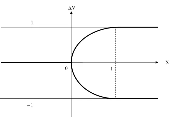
depicted in Figure 6.

Figure 6: Stable location equilibria

1

−

1

1

0 1

X

The result plotted in Figure 6 is clear. If transport costs are high (X is low),

the firms scatter in two equally sized groups each one being located in a different

region in order to sell to nearby consumers. If transport costs are high (X is low), the

firms export easily so that that they agglomerate in a region in order to exploit

economies of localization. For intermediate levels of transport cost, the firms

distribute themselves across the regions in an asymmetric way.

4.

Location of firms under vertical monopoly.

Up to now we have dealt with the location of firms that interact on the basis

that their products are substitutes (oligopoly models). However, firms also interact in

the location choices when their products are complements. This is the case of vertical

monopoly: an upstream firm U processes labor into an intermediate good that is sold

to a downstream firm D. This latter firm combines the input with labor in order to

manufacture a final product that is sold to consumers. The question that we pose here

is similar to the question concerning spatial oligopoly: do vertically-related firms tend

to choose separate locations in equilibrium or do they prefer to agglomerate?

In empirical terms, there are instances of both equilibrium strategies: in the

textile industry, manufacturing is shifted to low wage countries, while design and

marketing stay in developed countries; in engineering industries, such as the car

industry, production of components co-locates with assembly even though factor

intensities of both stages are very different.

The reference paper in this field is PAIS and PONTES (2008). The model

has the following assumptions. There are two countries called Home (H) and Foreign

(F). Country F has lower wages than H, so that w_H >w_F ≥0. On the other hand, the

purchasing power in country H exceeds the purchasing power in country F, this being

expressed by the fact that the number of consumers in H n, H,is higher than the

identical demand functions f

( )

p , where p represents the delivered price, and satisfies the following assumptions:

1. f is continuous and differentiable;

2. f is decreasing;

3. The maximum price = −1

( )

0

f

p is finite; 4. The total revenue function is strictly concave.

There are two vertically linked firms: the downstream firm

( )

D , producing a consumer good to be sold in both countries, and the upstream firm

( )

U , providing an

intermediate good to the downstream firm.

U transforms cU

(

cU ≥0

)

units of labor into one unit of the intermediate good

and D uses αunits of the intermediate good together with cd

( )

cd ≥0units of labor to

produce one unit of the consumer good. The parameterα, satisfying the condition

1

0≤

α

< , represents the intensity of vertical linkages.

Each firm carries its own product. The parameter t denotes the transport cost

of both products (final and intermediate) between the two countries. Transport costs

within each country are assumed to be zero. The assumption that transport costs are

the same between goods rests on the fact that they usually vary in proportion.

When D locates in country X_D and U locates in countryX_U, with the

condition XD,XU ∈

{

H,F

}

, firm D sets discriminatory prices

D

D X

F X

H p

p and in each

country, while firm U sets a delivery price _kXU_{for the intermediate good.}

With these assumptions, firm D’s profit function is

( )

( )

[

₍

₎

]

( )

p

[

p k c w t d

(

X F

)

]

And firm U’s profit function is:

( )

[

( )

( )

]

[

₍

₎

]

U D X

U X X F F X H H X

X

U n f p n f p k c w U t d X X

U D D

U

D, = ⋅ + ⋅ − ⋅ − ⋅ _,

Π α (7)

where d

(

X,Y

)

represents the distance between locations X and Y, with

{

H F

}

Y

X, ∈ ,

Firm D and Firm U play a non-cooperative three-stage game. In the first stage, firms

simultaneously choose their locations in the two-country economy. Given the adopted

locations, X_D and X_Uin the second stage, firm U sets _kXU _{, the price of the intermediate}

good. Finally, in the third stage, firm D quotes XD

H

p and XD

F

p , the prices for the final good in countries H and F, respectively.

The main results of the vertical monopoly can be described in Figure 7, where the

(H,F)

(F,F)

(H,H) and (F,F) t

(

H F

)

U w w

c −

α

(

)

F H

F H F H D

n n

n n w w c

− + −

(F,F)

(H,F)

Figure 7 shows several aspects of the location of vertically related monopoly

firms:

1. The fall of transport costs t to very low levels always leads to the

agglomeration of the upstream and downstream firm in the low labor cost country,

since the choice of locations is then driven by production costs only.

2. However, this process exhibits two distinct patterns depending on the

intensity of vertical linkagesα.

3. If α is low, the fall of trade costs may determine a transition from the

agglomeration in the large, high labor cost H to spatial fragmentation, where the

upstream firm locates in the small low labor cost country F and the downstream unit

D stays in the large, high labor cost market H. Further reduction of t leads eventually

to agglomeration in the small, low labor cost country F.

4. By contrast, if α is high, there are multiple agglomeration equilibria for high

values of transport cost t, since in this case the transport cost of the intermediate good

is high, and for each firm to cluster in either country is better than selecting an

isolated location.

5. Fragmentation of production is more likely to arise if the countries are very

5. Location of firms under monopolistic competition: agglomeration

of production under increasing returns.

KRUGMAN (1980) sets the foundations for the agglomeration of firms that

operate under increasing returns. He assumes that there are a large number n of

differentiated goods that have a constant elasticity of substitution. All consumers have

the same utility function:

n i i

U =

∑

cθ 0<

θ

<1 (8)

where c_i is the consumption of good i . Labor is the single production factor. All the goods have the same cost function:

i

i x

l =

α

+

β

α,β >0, i=1,…,n ₍₉₎

where l_i is labor used in the production of good i and x_iis the output of this good, so that there is a fixed cost and a constant marginal cost. Consequently, the

average cost declines for all levels of output and the firm operates under increasing

returns to scale.

The output of each good equals the sum of individual consumptions. We

identify the consumers with workers. Hence the output of good i is equal to the

consumption of a representative individual times the size of the labor force L:

i i Lc

It is assumed full employment, so that the labor force is equal to the total

labor used in production:

(

)

∑

=

+ = n

i

i x L

1

β

α

(11)

Finally, it is assumed that the firms maximize profits, but there is free entry

by firms, so that in equilibrium profits are always zero.

Under this setting, firms operate under Chamberlinian monopolistic

competition following the constant elasticity substitution version of

DIXIT-STIGLITZ (1977). This market structure has the properties outlined in page 25.

KRUGMAN (1980) then proceeds considering two identical countries

(regions) except in what concerns size (as measured by the labor force). He assumes

in a first step, that transport costs are zero. Even in this case, openness to trade

benefits the consumers in either country. Basically, trade determines that each variety

is produced in a single plant in a single country thus allowing the exploitation of

economies of scale. Increasing returns lead to more output, not in the form of a larger

scale of production of each good but rather through the increase of the number of

differentiated goods available to each consumer. It can also be shown that trade is

always balanced in this case.

Then positive transport costs are introduced in the trade between the two

countries. These costs have an “iceberg” form: if one unit of a good is exported from

a country to the other, only

τ

<1 arrives to destination, a share 1−

τ

disappearing in transit.3

If it is assumed that the size of the Home country in terms of the number of

workers/consumers is larger than the size of the Foreign country (L>L*), it can be

3

This assumption is made for the sake of simplicity and it ensures that the spatial price

proved that there is a “Home Market effect”: the former country becomes a net

exporter of the differentiated consumer goods. This follows from two considerations:

1. Given the existence of economies of scale, it always pays off to

concentrate the production of each variety in a single plant in a single

country.

2. With positive transport costs, it always pays to locate this single plant in

the larger market in order to avoid transport costs. The smaller market

can be supplied through exports.

However, under the assumption of immobility of workers/consumers across

countries, the trade flows between the two countries should be balanced. KRUGMAN

(1980) considers two possible ways of achieving this goal.

If there is a single class of differentiated goods, the smaller country can

produce and export an amount similar to its imports only if it has lower nominal

wages, i.e. lower production costs, than the large country.

If there are two classes of differentiated goods and demand is symmetrically

distributed, so that each country has a larger domestic demand in one class, trade

balance can be achieved with each country becoming a net exporter of that class of

goods. In this case, nominal wages are equal across the countries.

KRUGMAN (1991) goes further in this research line, by considering a

two-region economy with two sectors: agriculture, operating under constant returns and

perfect competition, and manufacturing, under increasing returns to scale and

monopolistic competition. Each sector has a specific factor: farmers in agriculture,

that are immobile; and workers in manufacturing, that are mobile across regions,

according to relative real wages. The output of agriculture is transported without costs

while the output of manufacturing bears an “iceberg” transport costτ . In this context,

the trade balance is not checked at an aggregate level but it rather follows from the

fact that for each kind of consumers there is a balance between her income and the

value of the output that it produces and sells in the global economy.

The “short run” equilibrium in this economy amounts to determining the

nominal wages in both regions given a regional distribution of workers across the

conflicting effects. On the one hand, the “Home Market effect” leads to higher

nominal wages in the larger region. On the other hand, we have an “Extent of

Competition” effect: more workers in a region mean a fiercer competition among

manufactured goods producers for the local market made by the farmers. It follows a

possible decrease of the nominal wages that the manufacturing firms can afford to

pay. The interplay of these two factors leads to an uncertain outcome.

However, the main focus of KRUGMAN (1991) is the determination of the

regional distribution of workers in the long run. Namely, it is sought whether in the

long run the manufacturing workers are either evenly dispersed across regions or they

instead agglomerate in one of the regions. It is assumed that workers move to the

region where real wages are higher, so that migration is sensitive to the relative real

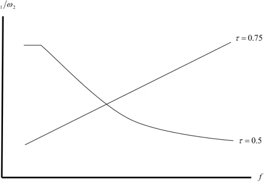
wage ω₁ ω₂.

Real wages are determined by nominal wages discounted by the price index of

manufactured goods. The price of the agricultural goods is irrelevant since it is the

same in both regions. The price index of manufactured goods is lower in the region

that contains more manufacturing firms and workers, as manufacturing goods bear

transport costs across regions. Hence, we have a “Price Index effect”: if more workers

and manufacturing firms enter a region, industrial goods become cheaper in that

region, increasing workers’ real wages and creating an incentive for the attraction of

more workers.

Hence, considering the possibility of geographic concentration versus

dispersion of manufacturing across the regions, the outcome is uncertain since we

have two centripetal forces (“Home Market effect” and “Price Index effect”) and a

centripetal force (“Extent of Competition effect”).

Basically, there will be regional convergence (dispersion of manufacturing) if

2 1 ω

ω decreases as a consequence of a movement of workers and firms from region

2 to region 1. And there will be regional divergence otherwise. This can be studied

numerically and KRUGMAN (1991) concludes that regional divergence obtains for

It is possible to confirm this result in an analytic way, although with a

slightly different meaning. Let us assume that all manufacturing firms and workers

are agglomerated in region 1. Then agglomeration is sustainable provided that no

firm finds profitable to “defect”, i. e., to shift to region 2. KRUGMAN (1991) finds

that three parameters matter for this decision:

1. The share of the manufacturing in expenditure and the allocation of

labor,

µ

. It increases the likelihood of regional concentration by two reasons: it increases the relative size of region 1 under spatial

concentration (“Home Market effect”); it decreases the relative cost

of living in region 1 (“Price Index effect”).

f

0.5

τ

=

Figure 8: Regional convergence and divergence

2 1 ω

ω

75 . 0

=

µ

2. The transport cost of the manufactured good, inversely given by τ . A

high value of τ (a low transport cost) has two contradicting effects: it

decreases the strength of competition for the local market of farmers;

it decreases the “Price Index effect”. KRUGMAN (1991) proves that

the first centrifugal effect predominates.

3. The strength of scale economies is inversely given by the parameter

θ

and it decreases the advantage of concentrating the increasing returns

sector in region 1.

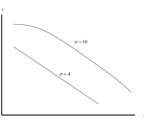
The combined influence of these parameters is depicted in Figure 9 in

( )

µ,τ

space, for given values of σ

(

σ =4andσ =10

)

.

τ

4

=

σ

10

=

σ

OTTAVIANO et AL. (2002) present a general equilibrium model of

geographical agglomeration that is very similar to KRUGMAN’s (1991). However,

several different assumptions lead to more simple and clear results. They assume that

the utility function of the consumers is given by (4) so that the direct demand

functions addressed to the firms are described by (5). Transport costs are not

“iceberg”, but they are expressed in units of numeraire. Together these assumptions

lead to a demand elasticity that varies with transport costs and according to the

number of firms located in a market. Consequently, prices are not a fixed markup of

costs but depend on the location of the firms. Prices are lower in the region where

firms agglomerate reflecting the intensity of competition.

The “Price Index” and “Extent of Competition” effects do not stem only

from the number of firms that locate in a region and thus avoid transport costs in

supplying that region, but they follow also from lower prices in that region as a result

of a higher intensity of competition.

This change of assumption gives the model a more realistic character and

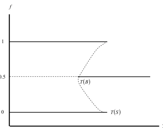
allows us to reach neater conclusions. KRUGMAN’s (1991) model had implicitly a

difference between the “sustain point”,T

( )

S , i.e. the level of transport costs above

which a full agglomeration of firms would be upset by a “defection” (a firm leaves the

cluster and sets up in the other empty region), and the “break-point”,T

( )

B , i.e. the

level of transport costs below which a symmetric distribution of firms becomes

unstable. Usually, the former point is higher than the latter (see Figure 10).4

4 _{Note that we are assuming now that}

τ

1

=

T , where τ is the amount of product that

arrives to destination if one unit is exported. Hence T is the amount that must be sent in order that one

Figure 10 depicts long run locational equilibria in

(

T, f

)

space, where

τ

1

=

T stands for the “iceberg” transport cost and f represents the share of workers

that live in a region. Thick lines plot stable equilibria and dashed lines represent

unstable equilibria, where stability means that a shift from the equilibrium is offset by

labor movements that restore the initial location pattern. In the KRUGMAN (1991)

economy, high transport costs

(

T higher than T

( )

S

)

lead the economy to a symmetric

division of manufacturing across the regions. By contrast, low transport costs

( )

(

Tlower thanT B

)

lead to a full agglomeration of increasing returns activities in one region. For intermediate transport costs

(

T

( )

B <T <T

( )

S

)

, there are multiple 0

1

T

( )

S T

( )

B T

5 . 0

f

equilibria, both dispersed and agglomerated, and this constitutes a weakness of the

model.

In OTTAVIANO et AL (2002), there is a unique threshold value of transport

cost T* such that T<T* entails agglomeration and T>T* leads to symmetric dispersion of manufacturing. 5The problem of existence of multiple patterns of

location does not exist. Furthermore this analysis is not bounded to the definition of

equilibrium spatial patterns, but allows us to make welfare considerations. Concerning

welfare, it can be said that:

1. For extreme values of transport costs, the equilibrium is coincident

with the socially optimum spatial pattern.

2. For intermediate values of T, the market discriminates against the

dispersion of manufacturing, thus leading to an excessive

geographical concentration.

6. Location of multi-plant (multinational) firms.

Up to now, we have assumed that each firm runs production activities in a

single point in space. In this section, we consider the location choices by firms

(multi-plant or multinational) that establish subsidiaries in regions (countries) different from

their home location, in the context of Foreign Direct Investment (henceforth named as

FDI).

The literature acknowledges two forms of FDI that differentiate according to

their relationship with trade and transport costs. On the one hand, the firm sets up a

plant in a foreign market in order to supply local consumers. By doing so, the firm

substitutes local production for exports from the home country, trading off the

5

Note that T means now a quantity of numeraire rather than an “iceberg” transport cost as in

benefits of proximity to final consumers (in the form of low transport costs) against

the advantages of geographic concentration of production (in the form of higher

economies of scale). This is clearly the type of FDI proposed by HORSTMANN and

MARKUSEN (1992) where trade and FDI are substitutes.

Another form of FDI consists in splitting the production process into several

vertically-related stages, each stage being intensive in a specific production factor.

For instance, the activity of the firm can be split in two parts: headquarters (intensive

in skilled labor) and plant (intensive in unskilled labor), that can be separated

spatially, each one being placed in a country abundant in the factor that is used more

intensively by that unit. This is clearly the form of FDI described by HELPMAN

(1984). In this case, FDI implies the existence of trade in intermediate goods and is

eased by low transport costs: trade and FDI complement each other.

The literature shows that the relationship between trade and FDI is not

simple (see, for instance, PAIN and WAKELIN, 1998). In PONTES (2007), a

non-monotonic relationship is proposed, inspired by BRAINARD (1993), of two

vertically-linked firms with different degrees of divisibility. It is assumed that the

upstream firm is indivisible and located in the home country. When the downstream

firm invests abroad, it eliminates the transport costs of the final product, but it has to

incur in the additional transport costs on the input that has to be imported from the

home country. This yields the possibility of a non-monotonic pattern.

We consider a location decision by a monopolist industrial firm in a spatial

economy made by two countries (regions): the home country, where the monopolist

headquarters locate and the foreign country where all final demand is located. Final

demand is described by f

( )

p , where p is delivered price. The demand function f

( )

p

exhibits the following properties:

1. It is continuous.

2. It is decreasing.