FUNDAÇÃO GETULIO VARGAS - FGV ESCOLA DE MATEMÁTICA APLICADA - EMAP
PROGRAMA DE PÓS-GRADUAÇÃO EM MODELAGEM MATEMÁTICA
ANTÔNIO LUÍS SOMBRA DE MEDEIROS
DEEP LEARNING FOR SINGLE IMAGE SUPER-RESOLUTION USING RESIDUAL IMAGE LEARNING AND MULTIPLE DEGRADATIONS
RIO DE JANEIRO, BRAZIL 2019
Antônio Luís Sombra de Medeiros
Deep Learning for Single Image Super-Resolution using
residual image learning and multiple degradations
Master Thesis presented to the School of Ap-plied Mathematics as partial requirement to obtain the Masters Degree in Mathematical Modeling
Fundação Getulio Vargas - FGV Escola de Matemática Aplicada - EMAp
Programa de Pós-Graduação em Modelagem Matemática
Supervisor: Dr. Eduardo Fonseca Mendes
Rio de Janeiro, Brazil
2019
Dados Internacionais de Catalogação na Publicação (CIP) Ficha catalográfica elaborada pelo Sistema de Bibliotecas/FGV
Medeiros, Antônio Luís Sombra de
Deep learning for single image super-resolution using residual image learning and multiple degradations/ Antônio Luís Sombra de Medeiros. – 2019.
65 f.
Dissertação (mestrado) -Fundação Getulio Vargas, Escola de Matemática Aplicada.
Orientador: Eduardo Fonseca Mendes. Inclui bibliografia.
1. Imagens em alta resolução. 2. Processamento de imagem. I. Mendes, Eduardo Fonseca .II. undação Getulio Vargas. Escola de Matemática Aplicada. III. Título.
CDD – 704.9
My flesh and my heart may fail, but God is the strength of my heart and my portion forever.
Abstract
Recent years have witnessed the unprecedented success of deep convolutional neural networks (CNNs) and Generative Adversarial Networks (GANs) applied in single image super-resolution (SISR) tasks. However, CNN-SISR based methods often assume that the lower resolution (LR) image is downsampled bicubicly from its high resolution (HR) counterpart. It results in poor performance on images with degradations that do not follow this assumption. Here, we propose a framework to learn a residual image super-resolver that handles multiple degradations, improving its performance on natural images. Our basic premise is that the residuals between an upsampled LR image and the HR counterpart contain information about the true degradation and downsampling processes, controlled by particular image features. We show that learning residuals in image space leads to detail reconstruction improvement in many cases.
In this work, we apply different CNNs/GAN-based models to learn and predict the residual image given the LR image. The residual to be learned is obtained by subtracting a bicubicly upscaled image of the LR image from the true HR image. The LR images are generated by applying a random blur degradation to the HR image followed by a bicubic downsampling. We also generate residuals from 3 different downsampling methods in LR image space dimensions to use as features. Finally, we show that our method is able to learn the spatially upsampled higher dimensional residuals and it can recover detailed HR images from bicubicly upsampled LR images by adding our proposed high resolution residual error.
Keywords: Super Resolution. Downsampling. Convolutional Neural Networks.
Resumo
Os últimos anos têm testemunhado o sucesso sem precedentes das redes neurais de convolucionais profundas (CNNs) e das Redes Generativas Adversárias (GANs) aplicadas em tarefas de super-resolução de imagem única (SISR). No entanto, os métodos de SISR baseados em CNNs/GANs geralmente assumem que a imagem de resolução mais baixa (LR) é subamostrada bicubicamente em relação à sua correspondente de alta resolução (HR). Isso resulta em baixo desempenho em imagens com degradações que não seguem essa suposição. Aqui, propomos um arcabouço de aprendizagem em que um super-resolvedor de imagem residual considera múltiplas degradações, melhorando o seu desempenho em imagens naturais. Nossa premissa básica é que os resíduos entre uma imagem LR sobreamostrada para alta resolução e a sua correspondente real de alta resolução contêm informações sobre os processos reais de degradação e subamostragem, controlados por características particulares da imagem. Mostramos que a aprendizagem residual no espaço da imagem leva à melhoria na reconstrução de detalhes em muitos casos. Neste trabalho, aplicamos diferentes modelos baseados em CNNs/GAN para aprender e prever a imagem residual dada a imagem LR. O resíduo a ser aprendido é obtido da subtração de uma imagem sobreamostrada bicubicamente da imagem LR de sua correspondente imagem real HR. As imagens LR são geradas aplicando uma degradação de borramento aleatório na imagem HR seguida de uma subamostragem bicúbica. Também geramos resíduos por 3 distintos métodos de amostragem em dimensões de espaço de imagem LR para usar como atributos. Finalmente, mostramos que nosso método é capaz de aprender os resíduos de maior dimensão espacial e pode recuperar imagens detalhadas de HR, a partir de imagens LR amostradas bicubicamente, adicionando o erro residual de alta resolução proposto.
Palavras-chave: Super resolução de única imagem. Múltiplas degradações.
List of Figures
Figure 1 – Differences of low resolution image generation frameworks used in syn-thetic dataset creation for training deep learning based supervised SISR
models. . . 20
Figure 2 – Difference of our method SISR method.. . . 21
Figure 3 – GAN framework . . . 24
Figure 4 – Conditional GAN framework for sketch to image of shoes translation. SOURCE: (ISOLA et al., 2017) . . . 25
Figure 5 – A general framework of SISR. . . 27
Figure 6 – General pipeline for the SRMD framework. . . 34
Figure 7 – Schematic of the dimensionality stretching strategy. For a LR image of size W × H, the vectorized blur kernel is first projected onto a space of dimension t and then stretched into a tensor M of size W × H × (t + 1) (we add one extra degradation map when we consider noise level). SOURCE: (ZHANG; ZUO; ZHANG, 2018) . . . 34
Figure 8 – Generator and discriminator of SRGAN with kernel size (k), number of feature maps (n) and stride (s) for each layer, e.g. the convolution layer k3n64s1 stands for 3x3 kernel filters outputting 64 channels with stride 1. The Source: (LEDIG et al., 2017) . . . 35
Figure 9 – A framework to obtain the real residual. . . 40
Figure 10 – A general framework for residual Super-Resolution. . . 40
Figure 11 – A general framework for multiple residuals SR. . . 42
Figure 12 – Visualization of isotropic and anisotropic Gaussian kernels with different kernel widths and rotation angles . . . 44
Figure 13 – Super-resolution results of the image “180000” (CelebA) with scale factor ×2. The second row shows the results for all the CNN models and the 3rd row shows the results for the GAN models. . . 46
Figure 14 – Super-resolution results of the image “180002” (CelebA) with scale factor ×2. The second row shows the results for all the CNN models and the 3rd row shows the results for the GAN models. . . 47
Figure 15 – Checkerboard effect on the SRGAN and SRGAN-randkern models. . . 48
Figure 16 – Super-resolution results of the image “180003” (CelebA) with scale factor ×2. The second row shows the results for all the CNN models and the 3rd row shows the results for the GAN models. . . 57
Figure 17 – Super-resolution results of the image “180004” (CelebA) with scale factor ×2. The second row shows the results for all the CNN models and the 3rd row shows the results for the GAN models. . . 58 Figure 18 – Super-resolution results of the image “180006” (CelebA) with scale
factor ×2. The second row shows the results for all the CNN models and the 3rd row shows the results for the GAN models. . . 59 Figure 19 – Super-resolution results of the image “180007” (CelebA) with scale
factor ×2. The second row shows the results for all the CNN models and the 3rd row shows the results for the GAN models. . . 60 Figure 20 – Super-resolution results of the image “180010” (CelebA) with scale
factor ×2. The second row shows the results for all the CNN models and the 3rd row shows the results for the GAN models. . . 61 Figure 21 – Specification of 6 VGG architectures. On this work use VGG19, the
List of Tables
Table 1 – Average results obtained by using CNN on test set. . . 45 Table 2 – Average results obtained by using GAN on test set.. . . 45
List of abbreviations and acronyms
SISR Single Image Super-Resolution CNN Convolutional Neural Network GAN Generative Adversarial Network
SRGAN Super-Resolution Generative Adversarial Network SRMD Super-Resolution for Multiple Degradations
Contents
1 Introduction . . . 19
1.1 Contextualization and Motivation . . . 19
1.2 Objectives . . . 21
1.3 Contributions . . . 22
2 Relevant Background. . . 23
2.1 Convolutional Neural Networks (CNNs) . . . 23
2.2 Generative Adversarial Neural Networks (GANs) and Conditional Genera-tive Adversarial Networks (cGANs) . . . 23
2.3 Image Super-Resolution . . . 25
2.3.1 Degradation Model . . . 26
2.3.2 Common downscaling methods . . . 28
2.3.3 Traditional SISR and Deep Learning in SISR . . . 28
2.3.4 Blind and Non-blind Models for Image Super-Resolution . . . 30
2.3.5 Image Quality Assessment . . . 30
3 Methods . . . 33
3.1 Baseline Models . . . 33
3.1.1 SRMD Model . . . 33
3.1.2 The SRGAN Model . . . 35
3.2 Loss Functions . . . 36
3.2.1 Content Loss (VGG loss) . . . 36
3.2.2 Adversarial Loss . . . 37
3.2.3 Residual Loss . . . 38
3.3 Proposed Frameworks . . . 38
3.3.1 Baseline with Random Blur Kernels . . . 38
3.3.2 Residual Image Frameworks . . . 39
3.3.3 Multiple Residual Images Frameworks . . . 41
4 Experiments . . . 43
4.1 The CelebA Dataset . . . 43
4.2 Training Data Synthesis . . . 43
4.3 Training Details . . . 44
4.4 Results . . . 45
Bibliography . . . 51
Appendix
55
APPENDIX A Result samples on the CelebA Dataset. . . . 57 APPENDIX B VGG architectures . . . 63
19
1 Introduction
This thesis presents two new frameworks for image super-resolution via residual learning using deep neural networks with application to the public benchmark dataset of face images CelebA(LIU et al.,2016). The motivation for learning residuals and combining them to CNNs and GANs models arises from the assumption that, the distribution of residual images with respect to a pilot super-resolver, in the high resolution space, is better behaved than the unconditional distributions of high resolution images, in a fixed domain. GANs have achieved good results on approximating distributions, and hence simpler distributions like the residual images of high resolution faces from bicubic upscaled low resolution faces can be learned by these neural networks methods. In this chapter, we present the problem, our objectives as well as the main contributions we have achieved.
1.1
Contextualization and Motivation
Image super-resolution is a highly challenging task that has a wide range of applications, such as face recognition, satellite image understanding, and medical image processing, to name but a few. Super-resolution has been an attractive research topic in the last two decades and has been very successful at low upscaling factors (2-4x) with Generative Adversarial Networks (GANs). The input to a super-resolution GAN is a low resolution image (e.g. 16x16 pixels in size). The output from the GAN is a higher resolution image (e.g. 64x64 pixels in size). Kim, Lee e Lee (2016a) adopted residual learning to address the problem of generating a high-resolution image given a low-resolution image, commonly referred as single image super-resolution (SISR). Another strategy proposed by Zhang et al. (2017) demonstrated that a single CNN model can handle multiple super-resolution scales, image deblocking and image denoising. Nevertheless, these approaches demand high computational cost due to the training step of deeper layers and the bicubic interpolation of low resolution images.
Despite impressive results in literature, recent deep learning methods still lack in practical applications, since they are normally trained in synthetic data sets. These datasets normally assume that a low resolution picture is generated via a deterministic downsampling method (LEDIG et al.,2017). As a matter of fact, real-world scenarios pose challenges for super-resolution because high resolution datasets are unvailable, downscaling methods are unknown and the input low resolution images are noisy and blurry (YUAN et al., 2018).
In order to recover high resolution images under the SISR approach, we employ different methods based on CNNs and GANs to learn high resolution residual images
20 Chapter 1. Introduction
given a low resolution image. The true high resolution residuals for training are obtained by subtracting a bicubicly upscaled image of the low resolution image of the true high resolution image. The set of low resolution images are generated by applying random blur degradations to the high resolution image followed by a bicubic downsampling. Our proposal also considers adding other image features to input the input data, e.g. residuals from 3 different downsampling methods in low resolution image space dimensions.
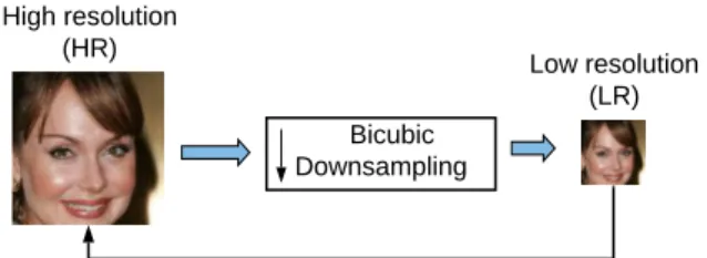
High resolution (HR)
Bicubic Downsampling
SISR: Recover HR from its bicubic downsampled LR counterpart
Low resolution (LR)
Current low resolution image generation framework for supervised training of SISR models
Low resolution (LR) Bicubic
Downsampling
SISR: Recover HR from its degraded and downsampled LR counterpart High resolution
(HR)
Our low resolution image generation framework (considering multiple degradations)
Figure 1: Differences of low resolution image generation frameworks used in synthetic dataset creation for training deep learning based supervised SISR models.
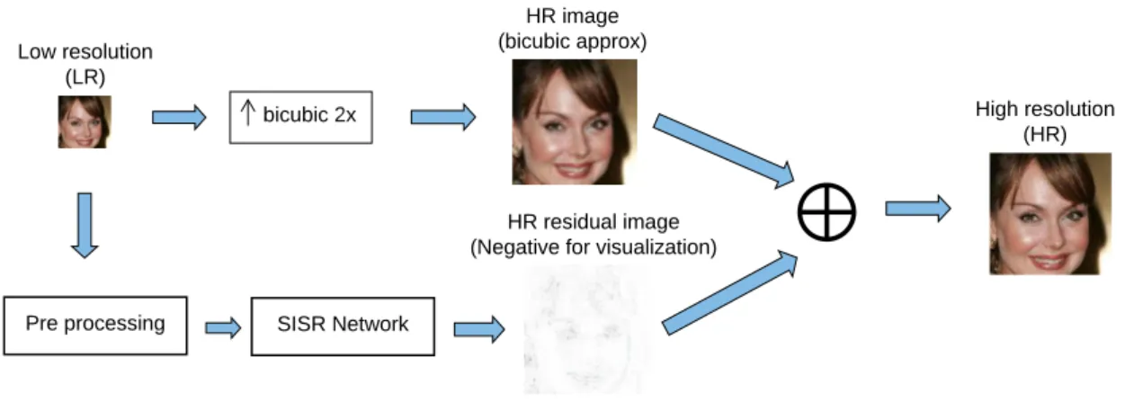
1.2. Objectives 21 SISR Network Low resolution (LR) High resolution (HR)
The current SISR framework retrieves a high resolution image from a low resolution image in an end-to-end manner
Low resolution (LR) High resolution (HR) bicubic 2x HR image (bicubic approx) HR residual image (Negative for visualization)
SISR Network Pre processing
Our SISR framework generates the residuals used to retrieve the high resolution image.
Figure 2: Difference of our method SISR method.
1.2
Objectives
This thesis develops a methodology based on SISR, CNN and GANs to upscale lower resolution images by learning its residuals from a pilot super-resolver. We apply these algorithms to the public faces dataset CELEB-A. To achieve this goal, the following specific objectives were drawn:
22 Chapter 1. Introduction
• Develop a super resolution method based on CNNs and GANs that takes synthesized training data by different degradations;
• Propose a residual image learning model for high resolution images to improve SISR tasks.;
• Evaluate and validate the proposed methods through experiments with real images.
1.3
Contributions
Our main contributions are:
• Development of a new blind single image super-resolution method based on residual image learning that also considers multiple degradations;
• Application of a GAN-based single image super-resolution model using multiple degradations;
• Performance evaluation of CNNs and GANs applied to SISR using different loss functions.
23
2 Relevant Background
This chapter presents the theoretical basis that supports the understanding of deep learning techniques for super resolution which focus on Convolutional Neural Networks and GANs. In fact, CNNs and GANs are the main architectures used to develop the proposed framework for Single Image Super Resolution (SISR).
2.1
Convolutional Neural Networks (CNNs)
CNNs are a special class of neural network (HAYKIN et al., 2009) developed for image application that comprise sets of layers for different purposes. The first layers extract local attributes from the input images, then deeper layers extract global attributes. The main purpose of this hierarchical organization is to provide the input signal passes through the successive layers, so that the position of the extracted attributes has less influence on the final output of the network (GOODFELLOW; BENGIO; COURVILLE, 2016).
The main difference from standard multilayer feedforward neural networks (HAYKIN et al., 2009, Chapter 4) is that CNN architectures explore spatial relationships of the input. The spatial structure of input images is explicitly used for regularization due to a limited connection between the layers. This is an advantage over fully connected networks, since for a network with the same number of layers it vastly reduces the amount of param-eters in the network. Other advantages of CNNs are the capability of extracting relevant features through kernel learning and special local invariance building neurons (pooling layers). These architectures effectively shifted the necessary engineering from design of handcrafted image features to the network connection structure and hyperparameter tuning (GOODFELLOW; BENGIO; COURVILLE, 2016).
The three main types of layers used to build Convolutional Neural Network archi-tectures are Convolutional Layer, Pooling Layer, and Fully-Connected Layer (LECUN et al.,1989). The layers are stacked together with different possible choices for the activation function to form a full architecture.
2.2
Generative Adversarial Neural Networks (GANs) and
Condi-tional Generative Adversarial Networks (cGANs)
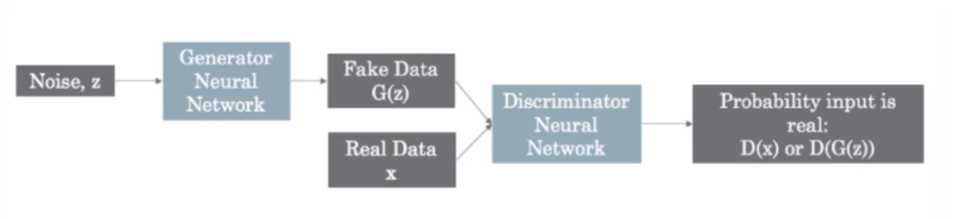
Generative adversarial networks (GOODFELLOW et al., 2014) are a framework for learning generative models based on the game theory. The main goal of GANs is
24 Chapter 2. Relevant Background
to train a generative network G(z; θ(G)) that produces samples approximating the data distribution, pdata(x), by transforming vectors of noise z as x = G(z; θ(G)). The training signal for G is provided by a discriminator network D(x) that is trained to distinguish samples from the generative distribution pG from real data (from distribution pdata). The generative network is then trained such that the discriminator accepts its outputs as being real. The G and D networks are trained in an adversarial manner by optimizing the adversarial expected loss:
V (G, D) = Ey∼pdata(y)[log(D(y))] + Ez∼pZ(z)[log(1 − D(G(z))], (2.1)
where y is the sample from the pdata distribution and z is a random encoding on the latent space. Then the optimal results for G and D will be achieved after doing
min
G maxD V (G, D). (2.2)
Figure 3: GAN framework
Several applications of GANs (DENTON et al., 2015; GOODFELLOW et al., 2014;RADFORD; METZ; CHINTALA,2016) have shown that they can produce excellent data samples. However, training GANs requires finding a Nash equilibrium of a non-convex game with continuous, high dimensional parameters (RADFORD; METZ; CHINTALA, 2016). GANs are typically trained using gradient descent techniques that are designed to find a low value of a cost function, rather than to find the Nash equilibrium of a game, what does not guarantee convergence. Empirically, it is equivalent to maximize log(D(G(z))) instead of minimizing log[1 − D(G(z))].
The first GAN used fully connected layer as its building block (GOODFELLOW et al., 2014). Later, Deep Convolutional Generative Adversarial networks (DCGANs) (RADFORD; METZ; CHINTALA, 2016) were proposed to use fully convolutional neural networks which perform better. Since then convolution and transposed convolution layers have become the core components in many GAN models. For more details on (transposed) convolution arithmetic, please refer the report in Dumoulin e Visin (2016).
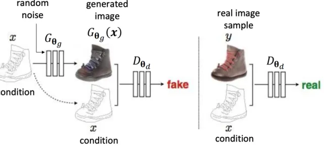
The original GAN could not control what would be generated, since its output relied on random noise. However, it can be added a conditional input y to the random
2.3. Image Super-Resolution 25
noise z so that the generated image is defined by G(z; y) (HUANG; YU; WANG, 2018). Typically, the conditional input vector y is concatenated with the noise vector z, and the resulting vector is part of the generator as it is in the original GAN. The meaning of the conditional input y is arbitrary, for example, it can be a class of image, object attributes or text descriptions of an image to be generated (HUANG; YU; WANG,2018). The modified adversarial expected loss for Conditional GANs is:
V (G, D) = Ex,c∼pdata(x,y)[log(D(x, y))] + Ey∼pdata,z∼pZ(z)[log(1 − D(y, G(z, y))]. (2.3)
Figure 4: Conditional GAN framework for sketch to image of shoes translation. SOURCE: (ISOLA et al., 2017)
2.3
Image Super-Resolution
The goal of super-resolution is to increase the resolution of an image. Resolution is a measure of frequency content in an image: high-resolution (HR) images are band limited to a larger frequency range than low-resolution (LR) images. In fact, the hardware required to process HR images is expensive. The resolution of digital photographs is limited by the imagery system. In conventional cameras, for example, the resolution depends on the CCD sensor density, which may not be sufficient to provide it. Likewise, infrared and X-ray devices have their own limitations. Super-resolution is an approach that attempts to resolve this problem with software rather than hardware.
Image super-resolution tasks generally take a low resolution image as input and outputs a high resolution one with sharp details. Early CNN based Super-Resolution methods aimed at minimizing the MSE error. Ledig et al. (2017) later introduced a single image super-resolution using a generative adversarial network (SRGAN) algorithm for
26 Chapter 2. Relevant Background
image super-resolution (SR) that uses a residual block (HE et al., 2016) based generator and a fully convolutional discriminator (RADFORD; METZ; CHINTALA, 2016) to do single image super-resolution. Besides adversarial loss, SRGAN also combines pixel-wise MSE (mean-square error) loss, perceptual loss (JOHNSON; ALAHI; FEI-FEI, 2016) and regularization loss (JOHNSON; ALAHI; FEI-FEI, 2016).
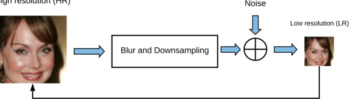
Super-resolution also refers to the task of restoring high-resolution images from one or more low-resolution observations of the same scene. It can be classified into Single Image Super-Resolution (SISR) and Multiple Image Super-Resolution (MISR). In the latter, multiple images are used to obtain one HR image (e.g. dictionary methods), whereas in the former the HR image is produced from a single LR image. High resolution images with high perceptual quality that present more valuable details and hence are relevant in many areas, such as medical imaging, satellite imaging and security imaging. Fig.5 exhibits a typical SISR framework and the LR image y is modeled as
y = (x ⊗ k) ↓js + n, (2.4) where x⊗k is the convolution between the blurry kernel k and the unknown HR image x, ↓js is the j downsampling operator (e.g. bicubic downsampler) with scale factor s, and n is the independent noise term. SISR is an ill-posed problem because one LR input may correspond to many possible HR solutions. The algorithms developed to solve SISR problems are mainly divided into three categories: interpolation-based methods, reconstruction-based
methods and learning-based methods.
2.3.1
Degradation Model
In order to approach the SISR problem, it is important to understand the degra-dation model which is not limited to Eqn. (2.4). Another practical degradation model is given by
y = (x ↓js) ⊗ k + n, (2.5) where ↓j
s stands for the j downsampler of scale factor s. Eqn. (2.5) corresponds to a deblurring problem followed by a SISR problem with bicubic degradation. Thus, it can benefit from existing deblurring methods and bicubic degradation based SISR methods. Still, the more widely assumed degradation model is given in Eqn. (2.4). In the following, we present the blur kernel k, noise n and downsampler ↓ that are part of Eqn. (2.4) and Eqn. (2.5).
• Blur Kernel:
The most popular blur kernel used in SISR is the isotropic Gaussian blur kernel parameterized by the standard deviation or kernel width (DONG et al., 2013; RIEGLER et al., 2015). In practice, other blur kernel models can be used such as
2.3. Image Super-Resolution 27
High resolution (HR)
Blur and Downsampling
Noise
SISR: Recover HR from its LR counterpart
Low resolution (LR)
Figure 5: A general framework of SISR.
the motion blur. Empirical and theoretical analysis (EFRAT DANIEL GLASNER, 2013; YANG; MA; YANG, 2014) have revealed that the influence of an accurate blur kernel is crucial for SISR. When the assumed kernel is smoother than the true kernel, the recovered image is over-smoothed. Most of the SISR methods actually favor for such case. On the other hand, when the assumed kernel is sharper than the true kernel, high frequency ringing artifacts will appear (DONG et al., 2013; RIEGLER et al., 2015).
• Noise:
The LR images are usually noisy and hence prior filtering may prevent noise ampli-fication by applying super-resolvers, directly to enhance resolution. However, the denoising pre-processing step tends to lose detail information and therefore deterio-rate the subsequent super-resolution performance (HUANG; SINGH; AHUJA,2015). Thus, it would be highly desirable to jointly perform denoising and super-resolution. • Downsampler:
According to (ZHANG; ZUO; ZHANG, 2018), the two most commonly considered downsamplers in literature are the direct downsampler (HE; SIU,2011;DONG et al., 2013) and bicubic downsampler (TIMOFTE; SMET; GOOL, 2014). Although the blur kernel and noise have been recognized as key factors for the success of SISR, it remains challenging to consider both blur kernel and noise, simultaneously, in a single
28 Chapter 2. Relevant Background
CNN framework. Riegler et al.(2015) also exploited the blur kernel information into the SISR model. Zhang et al (2018) considers a more general degradation framework and exploits a more effective way to parameterize the degradation model.
2.3.2
Common downscaling methods
Methods of downscaling (or downsizing) are downsampling techniques applied to images. There are a few traditional downscaling methods (PARSANIA; V.VIRPARIA, 2015) that are very common on the super-resolution literature (HAN,2013). Some of these methods are following defined.
• Nearest Neighbor downsampling: Nearest-neighbor downsampling is a degradation model that consists of a nearest-neighbor interpolation only. Nearest-neighbor inter-polation (also known as proximal interinter-polation or, in some contexts, point sampling) is a simple method of multivariate interpolation in one or more dimensions. Interpola-tion is the problem of approximating the value of a funcInterpola-tion for a non-given point in some space when given the value of that function in points around (neighboring) that point. The nearest neighbor algorithm selects the value of the nearest point and does not consider the values of neighboring points at all, yielding a piecewise-constant interpolant. .
• Bilinear downsampling: Degradation model consisting only of the downsampler technique based on bilinear interpolation, which is an extension of linear interpolation for interpolating functions of two variables (e.g., x and y) on a rectilinear 2D grid. The key idea is to perform linear interpolation first in one direction, and then again in the other direction. Although each step is linear in the sampled values and in the position, the interpolation as a whole is not linear but rather quadratic in the sample location.
• Bicubic downsampling: Degradation model consisting only of the downsampler technique based on bicubic interpolation. Bicubic interpolation is an extension of cubic interpolation for interpolating data points on a two-dimensional regular grid. It can also be used for upscaling, and in this case the interpolated surface is smoother than corresponding surfaces obtained by bilinear interpolation or nearest-neighbor interpolation (when both are used for upscaling).
2.3.3
Traditional SISR and Deep Learning in SISR
Learning-based SISR methods, also known as example-based methods, are brought into focus because of their fast computation and outstanding performance. These methods usually utilize machine learning algorithms to analyze statistical relationships between the
2.3. Image Super-Resolution 29
LR and its corresponding HR counterpart from substantial training examples. Inspired by the sparse signal recovery theory researchers applied sparse coding methods (TIMOFTE; SMET; GOOL,2014) to SISR problems. Meanwhile, many researches combined the merits of reconstruction-based methods with the learning-based ones to further reduce artifacts brought by external training examples (ZHANG et al., 2017).
Deep convolutional neural networks(DCNNs) have demonstrated outstanding per-formance in SISR. Dong et al.(2016a) introduced CNN to image Super-Resolution and demonstrated that deep learning can achieve higher quality image than other learning-based methods. They designed a simple fully convolutional neural network that directly learns an end-to-end mapping between low-resolution and high-resolution images (DONG et al., 2016a). Furthermore, they pointed out that the three convolutional layers can be abstracted into patch extraction and representation, non-linear mapping and reconstruc-tion, respectively. Several other models (LAI et al., 2017; KIM; LEE; LEE, 2016b) are presented to improve the performance of deep learning methods based on CNNs.
In general, the more layers the CNN model has, the better the model performance, but the deep model convergence speed becomes a critical issue during training. However, the very deep convolutional network (VDSR) proposed by (KIM; LEE; LEE, 2016b) which was based on residual learning (HE et al., 2016), can effectively strengthen the transfer of the gradient and enhance the convergence speed. In their model, the number of convolutional layers goes up to 20, while the model presented in (DONG et al., 2016a) only has 3 layers. Compared with Dong’s work (DONG et al., 2016a), VDSR achieves better performance not only on image quality, but also on the running time. Recently, Lai et al. (2017) proposed a Laplacian Pyramid Super-Resolution Network (LapSRN) based on a cascade of convolutional neural networks (CNN). The network progressively predicts the sub-band residual in a coarse-to-fine fashion and is trained with a robust loss function to reconstruct the high-frequency information.
Different from the previous works, generative adversarial network (GAN) is one of the most common methods (GOODFELLOW et al.,2014; LEDIG et al., 2017) suitable to be adapted to SR. GAN-based methods can generate HR images with much sharper details than other generative models(DENTON et al.,2015) In order to reconstruct more realistic texture details with large upscaling factors, Ledig et al. (2017) proposed a deep residual network with the perceptual loss function which consists of an adversarial loss and a content loss. Specifically, the authors calculated the content loss based on high-level feature maps of VGG network (SIMONYAN; ZISSERMAN, 2015) instead of MSE (the mean squared error).
30 Chapter 2. Relevant Background
2.3.4
Blind and Non-blind Models for Image Super-Resolution
Blind super-resolution algorithms consider the HR image and the degradation kernel unknown and try to recover both from the low-resolution image. Non-blind super-resolution algorithms assume the kernel to be known and only recover HR from both the kernel and low-resolution image. Normally non-blind super-resolution models are paired with some kernel estimation algorithm.
The estimation of the degradation of the blur kernel is an essential step for blind SR. Wang, Tang e Shum(2005) proposed a probabilistic framework combined with the image co-occurrence prior to estimate the unknown point spread function (PSF) parameters. According to the property that small image patches will re-appear in natural images, Michaeli e Irani (2013) presented a method that was able to estimate the optimal blur kernel. Another relevant work (SHAO; ELAD, 2015) introduced a convolution consistency constraint to guide the blur kernel estimation process, achieving state-of-the-art blind Super-Resolution performance.
Although a lot of works focus on Super-Resolution problems with known degrada-tion/downsamping kernels, only few works try to solve blind Super-Resolution problems considering that the degradation operators from HR images to LR images are unavailable. The problem with the best non-blind state-of-the-art models is that they not only assume the blur kernel to be known, but they also consider the same kernel for all training and test images. Thus, these methods are designed for a single blur kernel only, e.g. bicubic or isotropic Gaussian with fixed kernel width. Recent works adapted these tasks for different blur kernels, without requiring different training phases (RIEGLER et al.,2015; Zhang et al., 2017; ZHANG; ZUO; ZHANG,2018). Blind SISR approach has achieved state-of-art results using blur kernel estimation with synthetic images, however it did not accomplish similar results for natural images. In this work, we investigate how deep learning can benefit blind Super-Resolution problems.
2.3.5
Image Quality Assessment
Two classical measures that are often used to indicate the degree of image degra-dation are the mean squared error (MSE) and its related peak signal to noise ratio (PSNR)(WANG et al., 2004). However, standard image quality measures such as MSE do not agree with human visual perception. In order to tackle image quality assessment, Wang et al.(2004) developed the structural similarity index (SSIM). SSIM measures the similarity between two images, i.e. between two windows, and evaluates objectively the image quality traditionally performed with PSNR. It is a referenced index that quantifies the distortion of an image due to compression, blurring, noise, etc., when compared to its original counterpart.
2.3. Image Super-Resolution 31
The SSIM index calculated between x and y was introduced in (WANG et al., 2004) as:
SSIM(x, y) = (2µxµy + C1)(2σxy + C2)
(µ2
x+ µ2y+ C1)(σx2+ σ2y+ C2)
, (2.6)
where µx, µy, σ2x and σy2 correspond to the mean and variance values calculated for x and
y, respectively and σxy stands for the variability between x and y. C1, C2 and C3 are
variables that stabilize the division operation.
According to (SHEIKH; SABIR; BOVIK, 2006), PSNR is an excellent measure of image quality with low computational cost and therefore, PSNR is used, in general, for video quality evaluation. It is given by
PSNR = 20 log10(M AXI) − 10 log10(M SE), (2.7)
where M AXI represents the highest value of image intensity I, usually 255 and MSE is defined as MSE = 1 N M N X l=1 M X r=1 (x(l, r) − y(l, r))2, (2.8)
where N and M represent the number of rows and columns of the images and the variables
33
3 Methods
This chapter presents the main tools and techniques used to design our SISR method. The first section presents the baseline models which includes a CNN-based model called SRMD –Super-Resolution for Multiple Degradations– introduced in (ZHANG; ZUO; ZHANG, 2018) and a GAN-based model for super resolution, SRGAN (Super-Resolution GAN), developed by (LEDIG et al.,2017). Different from the Super-Resolution methods introduced with SRGAN and SRMD, our proposed learning algorithm makes use of these architectures to train blind models for multiple degradations, also taking the advantage of learning image residuals. Then, we present the loss functions which play a central role in CNN models. The last section describes the proposed method which deals with synthetized training data by using different degradations. Although we prefered to not consider explicit gaussian additive noise, it easy to add this feature if one wants to implement the full degradation framework.
3.1
Baseline Models
3.1.1
SRMD Model
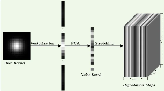
In this work, the noise-free method introduced in (ZHANG; ZUO; ZHANG,2018) is our CNN based-model and we refer to it as SRMD throughout the document. Zhang, Zuo e Zhang (2018) approached the SISR problem using trained Super-Resolution models on synthetic datasets and assuming only one type of degradation given a non-blind model. These authors also introduced a technique called dimensionality stretching to incorporate kernel information in input to training a CNN. The synthesis of LR images on this model follows the degradation model displayed in Figure 5. It consists in convolving the HR image with a random blur kernel and prior to downsampling it using a specific downsampling method (e.g. bicubic interpolation). The same blur kernel used to degrade the HR image on the process that generates the LR image is passed via degradation maps concatenated to the LR image as input during the training process. The dimensionality stretching strategy is described in Figure 7. It is performed by flattening the blur kernel into a vector and then reducing it to a smaller size via Principal Component Analysis (PCA). Each element of the reduced kernel vector is transformed into a degradation map by repeating it W × H times, where W and H are respectively the width and height of the LR image. Then, it is added as a channel to the image. Figure 6 exhibits a general sketch of this model, after the pre-processing step, i.e.the LR image generation from the HR image and the generation of degradation maps from the blur kernel to create the input for the model).
34 Chapter 3. Methods P ix e lS h u ff le 2 x c o n v + B N + R e L U c o n v + B N + R e L U c o n v + B N + R e L U c o n v + B N + R e L U . . . . . . c o n v + B N + R e L U c o n v HR image LR image with Degradation
Maps CNN
Figure 6: General pipeline for the SRMD framework.
00 00 00 Stretching Vectorization Blur Kernel PCA Noise Level t+1 Degradation Maps W H
Figure 7: Schematic of the dimensionality stretching strategy. For a LR image of size
W × H, the vectorized blur kernel is first projected onto a space of dimension t and then
stretched into a tensor M of size W × H × (t + 1) (we add one extra degradation map when we consider noise level). SOURCE: (ZHANG; ZUO; ZHANG, 2018)
3.1. Baseline Models 35
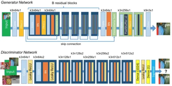
Figure 8: Generator and discriminator of SRGAN with kernel size (k), number of feature maps (n) and stride (s) for each layer, e.g. the convolution layer k3n64s1 stands for 3x3 kernel filters outputting 64 channels with stride 1. The Source: (LEDIG et al., 2017)
3.1.2
The SRGAN Model
SRGAN (LEDIG et al.,2017) was the first model to achieve visual realistic results for 4x single image super-resolution. It uses an adversarial approach and optimizes the content loss and adversarial loss instead of employing the MSE per-pixel error. Although it is able to produce extremely realistic images, its performance evaluation in terms of PSNR and SSIM metrics indicates that it does not outperform the previous models in literature. Since PSNR is equivalent to the per-pixel loss, a model trained to minimize per-pixel loss should outperform a model trained to minimize feature reconstruction (content) loss, when evaluating its results by using PSNR. There are studies (WANG et al., 2004; JOHNSON; ALAHI; FEI-FEI, 2016) in literature that assess PSNR and SSIM relating them to the human assessment of visual quality. Figure 8 illustrates the generator and discriminator architectures. The generator is inspired in the ResNet architecture (SZEGEDY; IOFFE; VANHOUCKE, 2017) and has residual blocks and skip connections. The discriminator is a CNN with fully connected layers at the end. In our experiments, we use an upscale factor of 2 (HR images have double width and double height compared to LR images), and we take out the last block that contains the Conv + Pixelshuffle + PReLU layers, since the original architechture, being used in a 4x upscale setting, had two Pixelshuffle2x upscaling layers.
36 Chapter 3. Methods
3.2
Loss Functions
Loss functions play a central role on the deep learning based models and their appropriate choice and definition may be key to a good performance. The loss lSR was initially based on the MSE loss function (DONG et al., 2016b). The disadvantage of this function is that it leads to over smoothed results and hence discards high frequency information. Later, the loss function lSR was adapted to a more sophisticated one that considered the perceptual similarity. This perceptual loss lSR, incorporated in the SRGAN model, was devised by Ledig et al. (2017). It comprises two parts, a content loss and an adversarial loss, since the SRGAN model uses an adversarial architecture. The perceptual loss function is given by:
lSR = lSRV GG | {z } content loss + 10−3lSRGen | {z } adversarial loss | {z }
perceptual loss (on SRGAN)
. (3.1)
In this work, we train a network to predict the residual in high resolution space and for this we add a new component to the perceptual loss: the residual loss. The residual loss is the MSE loss of the predicted high resolution residual and the true one.
The proposed lSR for our SRGAN based architecture is then defined as:
lSR = lSRV GG | {z } content loss + 10−3lGenSR | {z } adversarial loss + lResSR |{z} residual loss | {z }
our perceptual loss
. (3.2)
Moreover, we consider lSR = lSR
Res for our CNN based method.
3.2.1
Content Loss (VGG loss)
In the proposed model, instead of relying on pixel-wise loss, we use the content loss inspired by (GATYS; ECKER; BETHGE, 2015; BRUNA; SPRECHMANN; LECUN, 2016; JOHNSON; ALAHI; FEI-FEI, 2016) and applied in (LEDIG et al., 2017). The content loss, in this work, can also be defined as VGG loss. It is based on the ReLU activation layers of the pre-trained 19 layer VGG network introduced in (SIMONYAN; ZISSERMAN, 2015). The variable φ indicates the feature maps obtained by the 2nd convolutional layer (after activation) before the 2nd maxpooling layer within the VGG19 network, which are the feature maps that achieve the best results according to (LEDIG et al., 2017). Inspired by (ZHANG; ZUO; ZHANG,2018), our content loss is defined as the euclidean distance between the feature representation of a reconstructed image GθG(I
LR) and the reference image IHR.
The main characteristic that differentiates our method from the others is that our super resolved HR image is the result of adding our generated HR residual image, given
3.2. Loss Functions 37
as output of our network, to a LR image the bicubicly upscaled to HR space (IHR
bicub). This implies that our recovered HR image is given by ˆIHR = G
θG(Input
LR) + IHR
bicub. Therefore, when we use L1-norm, the content loss will be given by
lV GGSR = 1 W H W X x=1 H X y=1 |φ(IHR) x,y− φ( ˆIHR)x,y|, (3.3) If we use L2-norm, the content loss will be given by the expression
lSRV GG= 1 W H W X x=1 H X y=1
(φ(IHR)x,y− φ( ˆIHR)x,y)2, (3.4) where φ indicates the feature maps obtained by the 2nd convolutional layer. W and H stand for the dimensions (width and height) of the respective feature maps (after 2nd convolutional layer and before 2nd maxpooling layer) within the VGG network.
3.2.2
Adversarial Loss
The adversarial loss arises from the idea that the discriminator can perform as a learned loss function instead of using a fixed function designed carefully for a specific task. This is particularly important for image synthesis tasks whose loss functions are hard to be mathematically defined. In the super resolution task, it is hard to write down explicitly a mathematical formulation that evaluates how well an image resembles a human face in high resolution. Since each input may have many valid outputs, and samples in training set cannot cover all situations, it is inappropriate to only minimize the distance between synthetic and ground-truth images. Indeed, we expect that the generator learns the data distribution instead of memorizing training samples.
Although we can design feature-based loss functions that preserve feature con-sistency, instead of looking at raw pixel level (e.g. content loss), such loss functions are constrained by pre-trained image classification models. A question remains on which layers to pick for calculating feature loss when we switch to another pre-trained model.
A discriminator, on the other hand, does not require explicit definition of the loss because it learns how to evaluate a data sample as it trains against the generator. Thus, the discriminator is able to learn a better loss function given enough training data. Lower values for adversarial loss functions mean that the generator is better at creating IHR that fools the discriminator.
The generative loss lSR
Gen based on the probabilities of the discriminator DθD over all training samples as:
lSRGen = N X n=1 − log DθD(GθG(Input LR)). (3.5) Here, DθD(GθG(Input
LR)) is the probability that the reconstructed residual image
GθG(Input
38 Chapter 3. Methods
game of GANs, but we choose to define it as − log DθD(GθG(Input
LR)) instead of log[1 −
DθD(GθG(Input
LR))] (GOODFELLOW et al., 2014) in order to improve the gradient behavior during minimization.
3.2.3
Residual Loss
In this work we introduce the residual loss. This loss is the L1-norm or L2-norm of the per-pixel difference between the true HR image and super resolved HR image. The expression using L1-norm for the residual loss is desbribed as:
lSRRes = 1 W H W X x=1 H X y=1 |IHR x,y − ˆI HR x,y |. (3.6)
If we use L2-norm, the expression for the residual loss then becomes:
lResSR = 1 W H W X x=1 H X y=1 (Ix,yHR− ˆIx,yHR)2. (3.7)
3.3
Proposed Frameworks
The proposed method comprises 6 models, excluding the 2 baseline models (SRMD and SRGAN), three are based on CNNs and the other three are based on GANs. All of them are derived from the baseline frameworks. We can also divide the models in three categories: Baseline with random kernels, residual image Super-Resolution, and multi-residual image Super-Resolution models.
3.3.1
Baseline with Random Blur Kernels
We define variant methods from the baseline SRMD and SRGAN that aim to perform blind image super resolution considering different degradations. Our two methods introduced in this section are named SRMD with random kernels (SRMD-randkern) and SRGAN with random kernels (SRGAN-randkern).
The basic modification, we propose here, refers to the pre-processing and training step. We use the same CNN architecture on SRMD and the same GAN architecture on SRGAN. On the other side, we train them on pairs of LR/HR images of faces where the LR image is generated by degrading the HR image using a convolution with a random blur kernel (from a pre-defined list) followed by a bicubic downsampling.
Regarding the SRGAN-randkern, we only changed the LR image data synthesis method from the normal SRGAN framework, whereas for the SRMD-randkern we also changed the way we apply the blur kernel as input. For the SRMD-randkern training process, instead of choosing the correct degradation kernel to pass as input during training
3.3. Proposed Frameworks 39
(since the SRMD method is non-blind), we randomly selected a kernel from the blur kernel list to concatenate with the LR image via dimensionality stretching and use as input to the CNN. The proposed modifications, i.e. changes in SRMD settings, converts it into a blind model, which we call SRMD-randkern.
3.3.2
Residual Image Frameworks
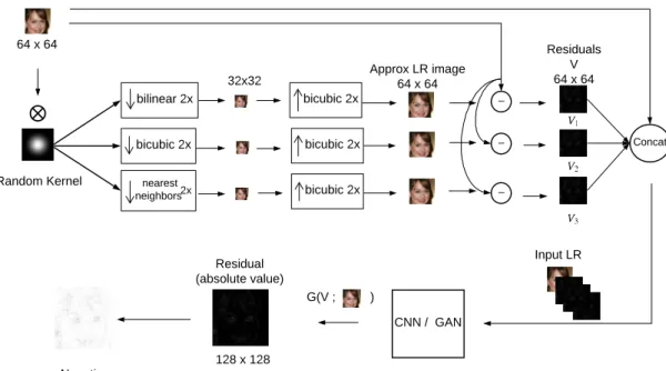
Our framework for residual learning consists of a model that predicts the residual image into the high resolution space. Within this framework there are two models: a CNN-based one namely SRMD for residual images (SRMD-resid) and a GAN-CNN-based method namely SRGAN for residual images (SRGAN-resid). Both models share the same idea and inherit the same underlying architectures of the baseline models. The pre-processing step considers the LR image generation using random blur kernels for our residual image models. Moreover, we include an additional step for residual calculation in the LR space to concatenate with the LR image in order to produce the input for our model. The process that generates the LR image and the HR residual images is illustrated in Figure 9. The LR residual image generation and the input generation for training our model is described in Figure 10.
We assume the HR image can be reconstructed from an upscaled image term y ↑bic and a residual image term r:
x = y ↑bic + r, (3.8)
where x is the HR image and, y is the LR image and r corresponds to the residual image, the error between the true HR image and the HR image approximated by upscaling the LR image bicubicly.
The real HR residual images are obtained by the procedure portrayed in Figure9. Since the residuals contain small and even negative values for pixels, we opted for using the absolute value followed by the negative of the residual image just for sake of better visualization.
In our framework, the LR image concatenated with a residual image in LR space is input to training our networks. We also train them on the real HR residual image and hence our model can learn to output residual images in the HR space. The LR residual image generation follows the steps described in Figure 10. The LR image is first degraded using a random blur kernel and then downsampled by selecting a downsampling technique at random (from a set of selected downsampling methods) to obtain a very low resolution image (VLR image). In this work, we restricted the set of downsampling methods to three: bilinear, bicubic and nearest neighbors interpolation. From the VLR image, we apply bicubic upscaling to recover an approximate LR image. Then, we subtract the bicubic upscaled approximation of the LR image from the real LR image which yields the residual
40 Chapter 3. Methods bicubic 2x bicubic 2x 128 x 128 128 x 128 HR image LR image HR image (bicubic approx) Negative 128 x 128 HR residual (absolute value) Random kernel
Figure 9: A framework to obtain the real residual.
in the LR space (LR residual V).
64 x 64 bilinear 2x bicubic 2x nearest neighbors 2x bicubic 2x 64 x 64 LR residual V LR image 32 x 32 LR image (bicub approx) Concat Random Kernel G(V ; ) CNN / GAN Negative 128 x 128
Residual (absolute value)
Input LR Random pick Downsampling
VLR image
64 x 64
3.3. Proposed Frameworks 41
Once obtained the input (LR image concatenated to LR residual image), we train our residual model by using any architecture based on deep learning. Here, we selected a CNN (SRMD model) and a GAN (from SRGAN).
Note that we used bicubic upscaling but our upsampling model can be extended to any deterministic technique to calculate the approximate HR image. After selecting the upsampling model, it is desirable to maintain the same method throughout our processing pipeline. The upscaling technique that generates the HR residual to train our model should be the same one for upscaling the VLR image and to generate the LR residuals. It is worth mentioning that we can use the same upscaling method on the LR image before adding the output of our model to generate our real HR image prediction.
3.3.3
Multiple Residual Images Frameworks
Another proposed method for general super resolution with residuals is the multiple residual. This method is similar to the aforementioned residual image framework, but it departs from the generation of our LR inputs.
Here, we define two other methods, based on CNN and GAN respectively, using this framework: SRMD with multiple residuals (SRMD-multiresid) and SRGAN with multiple residuals (SRGAN-multiresid). Our hypothesis is that, given more information from LR residuals, e.g., information from multiple downsampling techniques altogether, we improve the learning performance.
The main difference from the previous framework is that, as Figure11 shows, our input for the network is the concatenation of three different residuals (V1, V2 and V3) and
42 Chapter 3. Methods bilinear 2x bicubic 2x nearest neighbors 2x bicubic 2x G(V ; ) LR image 32x32 Approx LR image64 x 64 Residuals V 64 x 64 CNN / GAN Negative 128 x 128 Residual (absolute value) Concat bicubic 2x bicubic 2x 64 x 64 Input LR Random Kernel
43
4 Experiments
This chapter presents the dataset we have performed our tests, describes our experiments and discusses the simulation results.
4.1
The CelebA Dataset
We perform experiments on faces from the CelebFaces Attributes Dataset (CelebA) (LIU et al., 2015) which comprises 202,599 celebrity images. We employed the “aligned” version, which has been compiled from the original version of “in the wild”. Every image from CelebA is RGB of size 178×218 and contains all faces in the center of the frame. Here, we crop the images to 128×128 pixels, getting only the face regions.
4.2
Training Data Synthesis
Our LR data is synthesized from the original HR images (128×128 images) following Eqn 2.5 as shown in Figure 5, with blurring and downsampling only (except for when training the SRGAN, when we just used bicubic downsampling). Our experiments do not consider noise. The parameters of the degradation operators are the same for all images and we use the default implementation of the convolution operation from the multi-dimensional image processing module of the SciPy library(JONES et al.,2001). The blur kernels are randomly selected from a set of kernels.
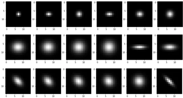
We select the same set of blur kernels for our experiments as in (ZHANG; ZUO; ZHANG, 2018), where a set contains a total of 342 blur kernels, comprising isotropic and anisotropic Gaussian kernels. The isotropic Gaussian kernels have fixed kernel width ranging in [0.2,2], sampling the kernel width by a stride of 0.1. The anisotropic Gaussian kernels, which are associated to a more general kernel assumption and furthermore expand the degradation space, are characterized by a Gaussian probability density function N (0, Σ) with zero mean and covariance matrix Σ (RIEGLER et al., 2015). The space of this type of Gaussian kernel is determined by the rotation angle of the eigenvectors of Σ and scaling of the corresponding eigenvalues. Zhang, Zuo e Zhang (2018) set the rotation angle range to [0, π] and they also set the scaling of eigenvalues from 0.5 to 6. The kernel size is fixed to 15×15.
Although we adopted the bicubic downsampler throughout the work to synthesize LR images, it is straightforward to train a model with other types of downsamplers. We can directly change the downsampler or, as Zhang, Zuo e Zhang(2018) argue for the case
44 Chapter 4. Experiments
Figure 12: Visualization of isotropic and anisotropic Gaussian kernels with different kernel widths and rotation angles
of the direct downsampler, we can change or include approximations of degradations with the direct downsampler to the blur kernel set. Specifically, given a blur kernel kd under the direct downsampler ↓d, we can find the corresponding blur kernel k
b under bicubic downsampler ↓b by solving the following problem with a data-driven method
kb = arg minkbk(x ⊗ kb) ↓ b
s −(x ⊗ kd) ↓ds k2, ∀ x. (4.1)
In order to use the dimensionality streching technique, we use the PCA projection matrix obtained for this blur kernel set, that, preserving about 99.8% of the data energy, it projects the 15×15 kernels onto a space of dimension 15. The visualization of some typical blur kernels is shown in Figure12.
Then, given a HR image, we synthesize the LR image by blurring it with a kernel
k and bicubicly downsampling it with a scale factor 2.
4.3
Training Details
Our implementation is based on PyTorch (PASZKE et al.,2017) and we trained all networks on a Nvidia Titan X Pascal GPU, using a sample set of 192,599 images from CelebA and cropped them to 128×128 in size. These images are distinct from the testing images and hence we performed our tests on a set of 10,000 images. Note that we can apply our models to images of arbitrary size as they are fully convolutional. During the training phase, we randomly selected a blur kernel to synthesize the LR image, depending on the
4.4. Results 45
model, and concatenating it along with the degradation maps to generate the network input. We scaled the range of the input to [0, 1] and the range of the output to [−1, 1].
We trained all models with 61,000 update iterations and used mini-batches of size 16. We experimented with L1 and L2 loss for per-pixel difference on the CNN models and with L1 and L2 for the content loss of GAN models. Our residual loss on the GAN models are always fixed as L2 per-pixel difference. We optimized each model’s loss function using Adam (KINGMA; BA, 2015) with β1 = 0.5 and β2 = 0.999. The learning is fixed to
10−3. For our GAN-based models we alternate updates to the generator and discriminator, which means k = 1 as used in (GOODFELLOW et al., 2014). During the test time we turned the batch-normalization off (IOFFE; SZEGEDY,2015). Following these settings, the training of each model takes about two days.
4.4
Results
Table 1 and Table 2 show the average values of SSIM, PSNR and MSE for the simulation results achieved with the CNN-based models and GAN-based models on the test set, respectively.
Table 1: Average results obtained by using CNN on test set.
Model Loss SSIM PSNR MSE
SRMD L1 0.838 26.682 176.719 L2 0.799 25.114 502.178 SRMD-randkern L1 0.917 31.252 61.521 L2 0.913 31.179 61.434 SRMD-resid L1 0.894 27.798 158.345 L2 0.894 27.663 163.278 SRMD-multiresid L1 0.890 27.339 175.589 L2 0.890 27.370 171.908
Table 2: Average results obtained by using GAN on test set.
Model Content Loss SSIM PSNR MSE
SRGAN L1 0.762 25.862 195.564 L2 0.694 24.670 245.871 SRGAN-randkern L1 0.438 19.039 828.393 L2 0.377 18.399 956.329 SRGAN-resid L1 0.865 26.391 193.701 L2 0.862 26.402 192.522 SRGAN-multiresid L1 0.861 26.382 192.960 L2 0.863 26,380 193.098
The CNN-based results demonstrated that our residual (SRMD-resid) and multi residual models (SRMD-multiresid) were capable of learning the residual images on the
46 Chapter 4. Experiments
(a) ground truth (b) bicubic PSNR/SSIM 27.430/0.813
(c) SRMD (d) SRMD-randkern (e) SRMD-resid (f) SRMD-multiresid 28.290/0.862 33.933/0.926 32.121/0.909 29.410/0.881
(g) SRGAN (h) SRGAN-randkern (i) SRGAN-resid (j) SRGAN-multiresid 25.379/0.685 19.785/0.394 28.413/0.872 28.276/0.876
Figure 13: Super-resolution results of the image “180000” (CelebA) with scale factor ×2. The second row shows the results for all the CNN models and the 3rd row shows the results for the GAN models.
HR space. In fact, these models recovered high frequency information or image details that effectively led to results close to the real HR image, since they achieved the highest SSIM values. The quantitative evaluation measures in Table 1confirmed the qualitative results present in Figure 13 and Figure 14. When comparing our results to the simple bicubic upscaled image, i.e. the original SRMD algorithm, we observe that the proposed residual-based models (SRMD-resid, SRMD-multiresid) improved the image result in Figure 13c.
It is worth noting that SRMD with random kernels (SRMD-multikern) showed unexpected results, since it outperformed the original non-blind model in terms of PSNR and SSIM. In fact, the non-blind model should perform better since the degradation model is known. Although considering simple blur kernels, we accomplished satisfactory results with our blind SRMD model. According to Zhang, Zuo e Zhang (2018), a blind model is not feasible to recover HR images when considering multiple degradations, particularly when the true degradation kernel is complex, e.g. motion blur kernel. Indeed, motion
4.4. Results 47
(a) ground truth (b) bicubic PSNR/SSIM 25.010/0.797
(c) SRMD (d) SRMD-randkern (e) SRMD-resid (f) SRMD-multiresid 28.369/0.898 34.438/0.967 27.776/0.914 27.079/0.890
(g) SRGAN (h) SRGAN-randkern (i) SRGAN-resid (j) SRGAN-multiresid 23.962/0.715 18.958/0.433 27.603/0.888 27.750/0.894
Figure 14: Super-resolution results of the image “180002” (CelebA) with scale factor ×2. The second row shows the results for all the CNN models and the 3rd row shows the results for the GAN models.
blur kernels are not part of our set of kernels. Our findings showed that learning a blind SRMD model with synthesized data for training and using multiple degradations can lead to competitive results when compared to the non-blind SRMD. As a matter of fact, the proposed blind model performed better than the non-blind SRMD in terms of SSIM and PSNR values (Table 1) as well as the visual quality of the recovered images (Figure 13, Figure 14). This led us to refute the statement that the generalization ability of the blind model, without a special designed architecture, is inferior to the non-blind and it furthermore performs poorly in real applications. Here, we employed simple architectures, available in literature, for CNN and GAN.
Regarding the GAN-based models, Table 2 shows the poor performance of the SRGAN with random kernels (SRGAN-randkern). It underperformed the other models in terms of SSIM and PSNR values and the visual results in Figure 13 and Figure 14. The low quality of the image results reached by the SRGAN-randkern can be explained by the artifact namely checkerboard effect which is remarkable in the results. This effect,
48 Chapter 4. Experiments
even less pronounced, can also be identified in the results attained with the SRGAN model shown in Figure 15. Researchers often face this issue when dealing with image synthesized by neural networks, and sometimes this can be solved by resizing the image (e.g. using nearest-neighbor interpolation) instead of using the deconvolution layer (e.g. a transposed convolution or PixelShuffle layer) at the end of the network. Another possibility to overcome this effect is to train the network for several epochs. We attempted both solutions but, although it diminished, it remained still noticeable.
SRGAN SRGAN-randkern
Figure 15: Checkerboard effect on the SRGAN and SRGAN-randkern models. The original SRGAN model, as expected, produced bad results, not only in terms of SSIM and PSNR, but in terms of perceptual quality. Overall, the results were over smoothed. This was due to the training using LR images generated by bicubic downsampled HR images. Therefore, the model learned only a type of inverse transformation for bicubic downsampling, producing low quality results when the image degradation did not follow this assumption.
For our residual models, the SRGAN-resid and SRGAN-multiresid did not perform very well against the CNN-based models. Our GAN-based models probably need more adequate losses to evaluate the image residuals and more careful hyperparameter tuning, since GANs are very sensitive to them. Nevertheless, we were able to confirm the potential of our generative adversarial networks model in modelling residual images. Since we decided to use one simple GAN-based framework for our experiments, we did not use any pre-trained network as initialization for the generator or applied any improved technique (SALIMANS et al.,2016) to training our GAN. Future works may lead the GAN-based framework to surpass the CNN-based one with other settings and training tweaks. More visual results can be found in Appendix A.
49
5 Conclusion
This thesis investigates the single image super-resolution problem on a more general setting: the low/high-resolution image pairs are not synthesized by a simple deterministic method. In general, the solutions available in literature assume that the lower resolution (LR) image is downsampled bicubicly from its high resolution counterpart. The proposed pipeline for SISR encompasses a degradation step with a random blur kernel before the bicubic-downsampling step to obtain synthetic LR images data. Here, the proposed approach learns a residual image super-resolver that handles multiple degradations given a LR image. Inspired by the recent successful image-to-image translation applications, we finally apply convolutional neural networks and generative adversarial networks to tackle this inverse problem and obtain the high resolution image. Overall, our approach leads to better results on synthetic data from the public CelebA dataset generated by different degradations, concerning quantitative and qualitative aspects. The experimental results demonstrate that the proposed method achieves comparable results as the state-of-the-art supervised models.
51
Bibliography
BRUNA, J.; SPRECHMANN, P.; LECUN, Y. Super-resolution with deep convolutional sufficient statistics. In: International Conference on Learning Representations (ICLR). [S.l.: s.n.], 2016. Cited on page: 36.
DENTON, E. et al. Deep generative image models using a laplacian pyramid of adversarial networks. In: Proceedings of the 28th International Conference on Neural Information
Processing Systems (NIPS) - Volume 1. Cambridge, MA, USA: MIT Press, 2015. p.
1486–1494. Cited 2 times on pages 24and 29.
DONG, C. et al. Image super-resolution using deep convolutional networks. IEEE
Transactions on Pattern Analysis and Machine Intelligence, v. 38, n. 2, p. 295–307, Feb
2016. ISSN 0162-8828. Cited on page:29.
DONG, C. et al. Image super-resolution using deep convolutional networks. IEEE
Transactions on Pattern Analysis and Machine Intelligence, IEEE Computer Society,
Washington, DC, USA, v. 38, n. 2, p. 295–307, fev. 2016. ISSN 0162-8828. Cited on page: 36.
DONG, W. et al. Nonlocally centralized sparse representation for image restoration. IEEE
Transactions on Image Processing, v. 22, n. 4, p. 1620–1630, April 2013. ISSN 1057-7149.
Cited 2 times on pages 26and 27.
DUMOULIN, V.; VISIN, F. A guide to convolution arithmetic for deep learning. arXiv
e-prints, p. arXiv:1603.07285, Mar 2016. Cited on page: 24.
EFRAT DANIEL GLASNER, A. A. B. N. A. l. N. Accurate blur models vs. image priors in single image super-resolution. In: International Conference on Computer Vision
(ICCV). [S.l.: s.n.], 2013. Cited on page: 27.
GATYS, L. A.; ECKER, A. S.; BETHGE, M. Texture synthesis using convolutional neural networks. In: Proceedings of the 28th International Conference on Neural Information
Processing Systems - Volume 1 (NIPS). Cambridge, MA, USA: MIT Press, 2015. p.
262–270. Cited on page: 36.
GOODFELLOW, I.; BENGIO, Y.; COURVILLE, A. Deep Learning. [S.l.]: MIT Press, 2016. <http://www.deeplearningbook.org>. Cited on page: 23.
GOODFELLOW, I. J. et al. Generative adversarial nets. In: Proceedings of the 27th
International Conference on Neural Information Processing Systems (NIPS) - Volume 2.
Cambridge, MA, USA: MIT Press, 2014. p. 2672–2680. Cited 5 times on pages 23,24, 29, 38, and45.
HAN, D. Comparison of commonly used image interpolation methods. Proceedings of the
2nd International Conference on Computer Science and Electronics Engineering, 03 2013.
Cited on page: 28.
HAYKIN, S. S. et al. Neural Networks and Learning Machines. [S.l.]: Pearson Upper Saddle River, NJ, USA:, 2009. v. 3. Cited on page: 23.