Cylindrical Spinning Rotor Gauge — A new approach for vacuum measurement

Pedro Gonçalo Dias de Almeida

Cylindrical Spinning Rotor Gauge —

A new approach for vacuum measurement

Dissertação para obtenção do Grau de Mestre em Engenharia Física

Orientador:

Orlando M. N. D. Teodoro, Professor Associado,

Universidade Nova de Lisboa

Júri:

Cylindrical Spinning Rotor Gauge — A new approach for vacuum measurement

Copyright cPedro Gonçalo Dias de Almeida, Faculdade de Ciências e Tecnologia,

Uni-versidade Nova de Lisboa

A

CKNOWLEDGEMENTS

Firstly, I would like to express my sincere gratitude to my advisor Professor Orlando Teodoro for giving me the chance to work in such an interesting project, for the stimulating discussions and his innovative ideas that made this dissertation so exciting.

Besides my advisor, I would like to thank everyone in the METROVAC laboratory for providing such a positive work environment, specially Nenad Bundaleski for the various insightful discussions and João Santos for his availability to help no matter how small the problem was.

I am grateful to José Carlos Mesquita for not only going to great lengths to make sure I always had the necessary resources available, but also for all the cake slices and for being a great company throughout the project.

I would like to thank João Faustino for his commentaries and the meticulous building of the first prototype parts in the physics department’s workshop. As well as Mr. Luís from the conservation and restoration department for the careful manufacture of the glass chamber.

My sincere thanks to the faculty’s library for making 3D printing available for everyone and specially to Filipe Silvestre for all the tips and for teaching me how to operate the 3D printer.

My gratitude to Mario Xavier for the help with the finite element method (FEM) simu-lations.

I would also like to thank my brother João Almeida who, besides being family with all that that entails, helped me troubleshoot some of the python code.

A

BSTRACT

The spinning rotor gauge (SRG) is one of the most interesting vacuum gauges ever made, covering a pressure range of over seven orders of magnitude, with minimal gas interference (no pumping, ionization or heating of the measured gas), and a great stability of less than 1% drift per year.

But despite its remarkable properties, apparently the SRG has not been further devel-oped since the eighties, when it gained commercial interest.

In this context, this dissertation aims at providing a starting point for a new line of investigation regarding this instrument, focused on the rotor itself.

A brief study of different rotor geometries is provided, including a comparison between a cylindrical rotor and a spherical one. A cylindrical spinning rotor gauge (CSRG) is then proposed, based on the original SRG, but requiring a completely new lateral damping system. A prototype was built and tested against a non calibrated reference gauge.

R

ESUMO

O spinning rotor gauge (SRG) é um dos manómetros de pressão mais interessantes devido ao facto de cobrir uma gama de pressões superior a sete ordens de grandeza, de não interferir com o gás medido (não bombeia, ioniza nem aquece o gás), e de ter uma estabilidade com variações inferiores a 1% por ano.

Apesar das suas excelentes propriedades, aparentemente o SRG não foi desenvolvido de forma significativa desde os anos oitenta, altura em que ganhou interesse comercial.

Neste contexto, esta dissertação procura providenciar as condições necessárias ao desenvolvimento de uma nova linha de investigação sobre este instrumento, com um foco no rotor deste.

É apresentado um breve estudo sobre diferentes geometrias, incluindo uma compara-ção entre rotores cilindricos e rotores esféricos. É proposto umcylindrical spinning rotor gauge(CSRG) baseado no SRG original, mas com um sistema de estabilização horizon-tal completamente novo. Foi construído um protótipo que posteriormente foi testado e comparado a um manómetro não calibrado de referência.

C

ONTENTS

Contents xi

List of Figures xiii

List of Tables xvii

1 Introduction 1

2 Magnetic Levitation Systems 3

2.1 Earnshaw’s Theorem . . . 4

2.2 Beyond the Earnshaw’s Theorem . . . 7

2.2.1 Diamagnetism . . . 7

2.2.2 Superconductivity . . . 8

2.2.3 Mechanical Constraints . . . 8

2.2.4 Non-static Arrangements . . . 9

2.2.5 Time-varying Fields . . . 10

2.2.6 Active Feedback Control . . . 11

3 The Spinning Rotor Gauge 15 3.1 Gauge’s Operation Principle . . . 19

3.1.1 Vertical Stabilization System . . . 19

3.1.2 Lateral Damping System . . . 20

3.1.3 Rotation System . . . 20

3.1.4 Rotor’s Frequency Detection . . . 20

3.2 Pressure Calculation . . . 21

3.2.1 Relative Deceleration Rate Evaluation . . . 23

3.3 Drag Sources and SRG’s limitations . . . 27

4 The Challenge of Low Pressure Measurement 31 4.1 Direct Pressure Measurement . . . 32

4.2 Indirect Pressure Measurement . . . 33

4.3 Calibration in the Low Pressure Range . . . 33

CONTENTS

5 Theoretical Considerations Concerning the Rotor 37

5.1 Pressure Calculation With a Cylinder Rotor . . . 38

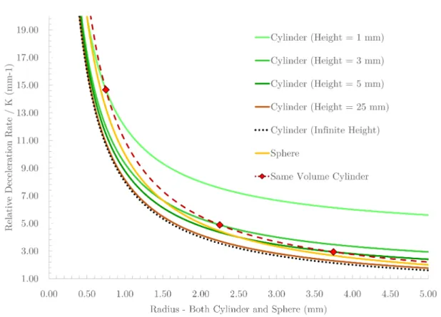
5.2 Cylinder vs. Sphere . . . 39

5.3 Other Properties . . . 42

5.3.1 Resistivity . . . 42

5.3.2 Thermal Expansion Coefficient . . . 43

5.3.3 Density . . . 43

5.3.4 Geometry . . . 44

6 Proposed Cylindrical Spinning Rotor Gauge 45 6.1 The Rotor . . . 45

6.2 Vertical Magnetic Suspension . . . 46

6.3 Lateral Damping . . . 51

6.4 Driving system . . . 58

6.5 Measurement . . . 62

6.6 Pressure Calculation . . . 63

6.7 Mechanical Considerations . . . 65

6.8 Vacuum Setup . . . 67

7 Results and Discussion 69 7.1 Magnetic Levitation Stability . . . 74

7.2 Lateral Damping . . . 76

7.3 Driving System . . . 77

7.4 Frequency Detection . . . 78

8 Conclusions and Future Perspectives 81

Bibliography 83

A Light Pressure 89

B Technical Drawings 95

L

IST OF

F

IGURES

2.1 Comparison between two electric fields, the dotted curves are equipotentials while the full curves represent lines of force [9]. . . 5 2.2 diamagnetic levitation of a frog [11]. . . 7 2.3 The Mendocino motor is a device designed around this concept [13–15]. . . . 8 2.4 a) diagram of the LevitronTM _{setup and b) diagram of the spin-precessing}

stabilization process [7]. . . 9 2.5 Four magnet segments of a Halbach array with respective magnetic flux lines. 10 2.6 Feedback levitation system diagram [18]. . . 11 2.7 Optical-based magnetic levitation system [19]. . . 12 2.8 Impedance-based magnetic levitation concept used by Fremerey in the SRG [18]. 12 2.9 Optical-based feed back controlled magnetic levitation [20]. . . 13

3.1 a) is a typical thread-based setup [30] and b) Holmes’ first magnetic levitation system proposal [8]. Where1and2identify the two levitation coils,Pa photo-cell,Sa source of light,La focusing lens, with a vaneVattached toNand a damping plateD. . . 15 3.2 Diagram of the Beam’s record holder magnetic levitation system [31]. BeingL1

the position sensing coil,Rthe rotor,Sthe levitation coil,Ia hollow magnetic core,Vthe vacuum connecting tube,Dthe driving coils and the needleH, the wireNand the glass tubeGform the lateral damping system. . . 16 3.3 a) is a photography of rotors bent and shattered by McHattie and b) a diagram

of the magnetic levitation system he used [37]. . . 17 3.4 a) diagram of the diamegnetic levitation concept and b) top-view diagram of

the torque delivery system [12]. . . 17 3.5 The spinning rotor gauge [42]: R - rotor; V - vacuum enclosure; M - one of two

permanent magnets; A - one of two coils for pickup and control of axial rotor position; L - one of four coils of lateral damping system; D - one of four drive coils; P - one of two pickup coils. . . 19 3.6 Diagram of a collision of a molecule with the SRG rotor rotating clockwise

LIST OFFIGURES

3.7 Diagram of a collision of a molecule with the rotor. . . 22

3.8 Simple frequency averaging [42]. . . 25

3.9 Multiple-track multiperiod averaging method [42]. . . 25

3.10 Multiple-track multiperiod averaging method with time separation∆t[42]. . 26

3.11 Accumulated multiperiod averaging [42]. . . 26

3.12 Accumulated multiperiod averaging with time separation [42]. . . 26

3.13 Isogai’s results from 18 independent measurements comparing eddy current plus electrostatic force with thermal effects in the SRG output. . . 28

3.14 Non-linearity curve for higher pressures [51]. . . 28

4.1 The pressure range of several manometers [53]. . . 32

4.2 Double-sided capacitance manometer [53]. . . 32

4.3 Example of a continuous expansion calibration apparatus [55]. . . 34

5.1 Relative deceleration rate (inmm−1) comparison of a sphere and cylinders of different heights, where the radii at which the volume of each cylinder is the same as the sphere’s is identified by the red marks and the red dashed line marks the respective trendline. . . 40

5.2 The ratio between deceleration rates of the cylinderDcand the sphereDs, for a given ratio of cylinder radiusrcover the sphere radiusrs. Where the heigh of the cylinder is defined as to keep the volume of the cylinder equal to the sphere’s by equation 5.18. . . 42

5.3 Diagram of a cylindrical rotor composed of two concentric cylinders of different materials. . . 44

5.4 Examples of alternative rotor geometries that would improve the trade-off between the surface of interaction with the gas and the moment of inertia. . . 44

6.1 Rotor’s available vibration movements wherezis the symmetry axis [18]. . . 45

6.2 Diagram of magnetic suspension setups. On the left, the first type of magnetic suspension implemented, and on the right, the system chosen for the final prototype. . . 47

6.3 Magnetic suspension control circuit. . . 47

6.4 At scale cutaway view of the support parts for the LED, on the left, and for the phototransistor, on the right. . . 48

6.5 Detail of the phase lead network used in the magnetic suspension circuit, in the figure 6.3. . . 48

6.6 Bode Plot of the phase lead network. . . 50

6.7 Finite element method (FEM) analysis comparison between simple magnetic suspension and magnetic suspension with a magnetic circuit where different colors represent different magnetic field magnitudes and the dashed red box represents the rotor’s position. . . 51

6.8 Diagram of magnetic suspension setups with lateral damping. . . 52

LIST OFFIGURES

6.9 Block diagram of one Hall sensor pair and respective damping coil pair

sub-system. . . 53

6.10 The electric circuit corresponding to one of the lateral damping subsystems. . 53

6.11 Offset and delay auxiliary circuits to the main circuit in figure 6.10. . . 54

6.12 FEM simulation of the lateral damping system offset’s impact in the overall magnetic field shape, where the black lines represent magnetic equipotential lines. The generated magnetic field is denominated as supporting if it con-tributes to the levitation of the rotor and opposing if it makes the levitation more difficult. . . 55

6.13 Torque in arbitrary units from the passive stabilization for several rotor angles with and without the magnetic circuit (MC). . . 55

6.14 Complete lateral damping system circuit, with the four subsystems. . . 57

6.15 Typical induction-motor speed-torque characteristic [56]. . . 58

6.16 Typical induction-motor speed-torque characteristic [56]. . . 58

6.17 Simplified two-pole machine: a) elementary model and b) vector diagram of the induced waves [56]. . . 59

6.18 Rotation driving circuit. . . 60

6.19 Generic layout of the system. . . 60

6.20 Diagram of the prototype’s different systems. Every component is identified by a code used in the different circuit schematics in figures 6.3, 6.9, 6.10, 6.14 and 6.18. . . 61

6.21 Rotation frequency measurement circuit. . . 62

6.22 Example of the shape of a TTL signal with the rotor’s frequency of rotation ready for data acquisition. . . 62

6.23 The different stages of the measurement process of the instrument. . . 63

6.24 SolidWorksTM3D render of all the built parts of the system. . . 65

6.25 SolidWorksTM 3D rendered exploded view. 1 rotor; 2 glass enclosure; 3 -upper body*; 4 - lower body*; 5 - -upper lid*; 6 - lower lid*; 7 - magnetic circuit; 8 - two identical upper and lower coil supports*; 9 - one of four drive coil supports*; 10 - cylindrical holders of the LED-phototransistor of the vertical stabilization circuit (* 3D printed parts). . . 66

6.26 SolidWorksTM 3D rendered cutawy views. 1 - rotor; 2 - lateral stabilization coil slots; 3 - Hall sensor slots; 4 - LED-phototransistor pair slots; 5 - vacuum entrance. All the rest vacant space was used for the necessary wiring. . . 66

6.27 Diagram of the vacuum system. . . 67

LIST OFFIGURES

7.2 Fremerey’s SRG normalized characteristic curve of relative deceleration (Ω= (−ω˙/ω)/(−ω˙/ω)sat) vs pressure (Π= p/psat) [42]. . . 71 7.3 Angle tolerance of the spinning rotor gauge [57]. . . 72 7.4 Eddy current induction drag dependence on the angle of the SRG’s head. . . 73 7.5 Output signal of the vertical stabilization circuit (TP node in figure 6.3) with

no rotation. . . 74 7.6 Output signal of the vertical stabilization circuit (TP node in figure 6.3) with

lower levitation coil turned on and no rotation. . . 75 7.7 Output signal of the vertical stabilization circuit (TP node in figure 6.3) with a

rotating rotor and with the driving system shut off. . . 75 7.8 The rotation signal, In black, is compared to the lateral damping signal, in

orange, at 400 Hz. . . 76 7.9 Measurement of the impact of the horizontal damping in the pressure readings. 77 7.10 Acceleration of the rotor from 100 Hz to the upper frequency limit around 750

Hz. . . 78 7.11 Optical signal of the rotation frequency at different frequencies. . . 79

A.1 Diagram of a light-based torque delivery method for the rotor of a CSRG. . . 89 A.2 Photon incidence with two possible outcomes: a) photon reflection and b)

photon absorption. . . 90 A.3 Incidence of light for torque delivery where a) represents the different force

components of one photon collision and b) the incidence of light with other important parameters for the torque calculation. . . 90 A.4 Three different configurations of the driving system. a) with just one system, b)

with two systems and c) with four. . . 93 A.5 Terminal angular frequency of a cylindrical rotor driven by a light pressure

based mechanism. . . 93

L

IST OF

T

ABLES

3.1 World record rotation speeds obtained by Beams in 1946 [31]. . . 16 3.2 Summary of the different SRGs built over time with the respective authors.

Adapted from Fremerey’s state of the art analysis in 1982 [30]. . . 18

4.1 Pressure categories according to the United Kingdom’s National Measurement Institute [52]. . . 31

6.1 Values of the parameters of the prototype relevant for the pressure calculation. 63

G

LOSSARY

c average molecular speed.

Ψ energy potential field.

ε vacuum permittivity.

ω angular frequency.

θ polar angle.

φ azimuth angle.

σ momentum accommodation coefficient.

τ the time needed for the rotor to complete a predefined number of turns.

ρ density.

γ electrical conductivity.

χe electric susceptibility.

εr relative permittivity.

µr magnetic permeability of free space.

A area.

B magnetic flux density.

E electric field.

F force.

Fe electric force.

Fm magnetic force.

H magnetic field.

I moment of inertia.

GLOSSARY

L angular momentum.

M molecular mass.

P polarization.

PEC power loss by eddy current.

R molar gas constant.

S surface.

T temperature.

V volume.

a relative proportion of each gas of the measured pressure.

c speed of light.

d distance to the axis of rotation.

f frequency.

h cylinder height.

m mass.

p pressure.

pl light pressure.

pm dipole moment.

q electric charge.

r radius.

t time.

z cylindrical longitudinal coordinate.

CSRG cylindrical spinning rotor gauge.

FEM finite element method.

LED light-emitting diode.

PLA Polylactic acid, a biodegradable thermoplastic aliphatic polyester.

SRG spinning rotor gauge.

TTL transistor to transistor logic.

C

H

A

P

T

E

R

1

I

NTRODUCTION

Vacuum technology has been established for a long time, from the industry to scientific research. Scientifically, it is a very old subject but its technology keeps on pushing the boundaries of what is possible to achieve. A good example of this evolution are the particle accelerators, where ultra high vacuum has to be sustained continuously for incredibly large volumes. Besides these outstanding systems, there are aspects of the technology that can be improved like cost, easy maintenance, reliability, etc.

In this context, the spinning rotor gauge is one of the most interesting pressure gauges. It has an incredible pressure range of operation that can theoretically go from 10−7_mbar

up to atmospheric pressures. Also, this gauge does not heat up the gas molecules in the measuring process, nor does it pump the gas, ionise its particles or change its properties in any other way; which alone is enough to make it more interesting than many other competing gauges.

Unfortunately, according to the literature there were no significant developments in this field of research ever since this instrument gained commercial interest in the eighties.

Not only could the commercial units still be improved by broadening their operation range to higher and lower pressures or increasing the instrument’s reading rate, for example, but there is also interest in using this instrument to investigate other physical phenomena.

CHAPTER 1. INTRODUCTION

Radiation pressure effects have already been reported by Fremerey [2], and one of the starting motivations behind this project was to see if it was possible to accelerate the rotor by applying tangential radiation pressure to it. Other interests include testing other rotors with possibly different geometries or composed by more than one material.

Such developments can only take place after the construction of a prototype. With future improvements like these in mind, the proposed prototype makes use of a cylindrical rotor instead of a spherical one, which alone required a whole new lateral stabilization system based on Hall sensors. Therefore, this dissertation is aimed at providing a starting point for a new line of investigation regarding this pressure gauge.

A study of the working principles is provided followed by the proposition and conse-quent implementation of a working prototype. In the end, pressure measurements were performed and compared with a reference gauge.

C

H

A

P

T

E

R

2

M

AGNETIC

L

EVITATION

S

YSTEMS

Magnetic levitation is far from being a trivial achievement. At first glance, one could assume that a carefully arranged static set of magnets could repel a smaller magnet in such a way that would allow stable suspension, but in fact, this is not possible.

This is known as the Earnshaw’s theorem [3]. It was published in 1849 by Samuel Earnshaw, who proved that it is impossible to achieve a stable static configuration of particles solely based on each other’s inverse-square law forces. Gravity and electromag-netism fall into such category, which at the time held many implications in the structure of the universe as it was then understood, and raised fundamental questions concerning the atom’s internal composition that would only be answered with the development of relativity and quantum mechanics.

Notwithstanding its consequences, this theorem makes certain assumptions that can be bypassed making magnetic levitation possible under special conditions. These cases include superconductivity [4], diamagnetism [5], mechanical constraints (or pseudo-levitation) [6], non-static arrangements (such as the levitron [7]), time-varying fields, and also the solution used by the spinning rotor gauge, active feedback control [8].

CHAPTER 2. MAGNETIC LEVITATION SYSTEMS

2.1

Earnshaw’s Theorem

One way to state this theorem is to say that no stable equilibrium can be attained by a particle in any sum of energy potential fieldsΨof inverse-square law forces.

For a stable equilibrium to occur, two necessary conditions must be met.

1.In the equilibrium point the net force must be zero.

∑

∑

This would be sufficient for equilibrium, but not enough for stability. Hence the need for a second condition.

2. If a particle subjected to the aforementioned force field was to be placed in the

said equilibrium point, there would have to be an arbitrary small vicinity around that point where the force points inwards as to oppose any displacement, independently of its direction.

In other words, the equilibrium has to be located in a relative minimum of the potential field.

∇2

∑

However, this condition cannot be satisfied since this kind of potential satisfies the Laplace equation [9].

∇2

∑

Therefore, no minimum points can exist in the potential of a inverse-square force. Equilibrium points do exist, but only as saddle points.

Gauss’s law can be used to illustrate this property in electric fields, and given that the conclusion also applies to magnetic fields, it will help characterize the limitations this theorem entails for magnetic levitation and the respective workarounds.

An electrostatic field that fulfils the requirements stated in equations 2.1 and 2.2 would have equipotential lines surrounding the minimum point, and force lines perpendicular to them. In the case of a positive charge, the force lines would have to point inwards as to provide the restoring force (as seen in the figure 2.1a), and in the case of a negative charge, they would have to point outward.

The field represented in figure 2.1a results from the requirements stated for the exis-tence of a minimum value in the electrostatic potential. As such, this field is impossible to occur as it would mean that flux lines would disappear in the minimum point without the presence of a charge, which goes directly against Gauss’s law.

2.1. EARNSHAW’S THEOREM

(a) Impossible situation where P is a minimum point

(b) Realistic situation where P is a saddle point

Figure 2.1: Comparison between two electric fields, the dotted curves are equipotentials while the full curves represent lines of force [9].

In such a field, if a Gaussian surfaceSof spherical shape is centred at the minimum point, and given that the electric field Epoints inwards, Gauss’s law will result in the following

Z Z

E·dS<0 (2.4)

where dSis an outward-oriented infinitesimal surface area element of the Gaussian sphere. From the divergence theorem, this implies the existence of a charge inside the surface.

Z Z

E·dS=

Z Z Z

∇·EdV= q

ε <0 (2.5)

Meaning that it is impossible to create a minimum in an electric field potential, and that imposing the stability criteria on an electric field results in the necessity of a charge being present in the aforementioned (and supposed vacant) minimum point, in order to comply with Gauss’s law.

Until now everything was done with particle charges in mind, but the proof stands for dipoles [10].

A dielectric body located in an electrostatic fieldEsuffers a polarisationPdictated by the body’s electric susceptibilityχe.

P= χeE (2.6)

From which the dipole moment pmmay be calculated over the volumeVof the body.

pm= Z

PdV (2.7)

pm = Z

CHAPTER 2. MAGNETIC LEVITATION SYSTEMS

This last equation’s integral can be simplified by assuming that the dipole is small enough for the electric field to be constant.

pm =χeEV (2.9)

The dipole moment is then used to calculate the force generated on the body.

Fe= (pm·∇)E (2.10)

Fe=χeV(E·∇)E (2.11)

The electric susceptibility is defined byχe =ǫr−1 whereǫris the relative permittivity of the material, and mathematically(E·∇)E= 12∇E2.

Fe = 1₂(ǫr−1)V∇E2 (2.12)

The force acting on the dipole can be analysed in the context of the stability criteria, namely the condition expressed by equation 2.2.

∇2Ψ_{e =−∇Fe} > 0 (2.13)

−∇

₁

2(ǫr−1)V∇E2

> 0 (2.14)

Yet the volumeV, the electric susceptibility(ǫr−1)and the term ∇E2 are always positive values, making this inequality impossible and thus confirming the Earnshaw’s theorem for electric dipoles.

Analogously to the electric force in equation 2.12, it is possible to write the magnetic force acting on a magnetic dipole [10].

Fm = 1

2(µr−1)V∇H2 (2.15)

To which the same stability criteria is applicable.

−∇

₁

2(µr−1)V∇H2

>0 (2.16)

And although the same reasoning applies to the volumeV and the term∇H2, the magnetic susceptibility(µr−1)is different since it can in fact be a negative number for a number of magnetic effects including diamagnetism, superconductivity and eddy current induction. Meaning that it is possible for these type of systems to find a stable configura-tion.

2.2. BEYOND THE EARNSHAW’S THEOREM

2.2

Beyond the Earnshaw’s Theorem

The conclusion that magnetic levitation is possible does not mean that Earnshaw’s theorem has exceptions. In fact, the reason why these types of magnetism are able to overcome its limitations is because they do not act as typical inverse-square laws.

2.2.1 Diamagnetism

Diamagnetism is a very subtle magnetic effect that is way less pronounced than paramag-netism or ferromagparamag-netism. It results from a change in the electrons orbital velocity due to an external magnetic field in accordance to Lenz’s law. In absence of an external magnetic field affecting the electrons of the material, a pure diamagnetic material will not show any signs of having magnetic properties.

Given its nature, this type of material acts as if it wants to expel the magnetic field within itself, hence the relative permeability being less than one. The magnetic field produced is dependent on the orientation of the external magnetic field, and the force produced will always be repulsive.

For this system

∇2B2 ≥0 (2.17)

Which means that a stable configuration is actually possible to achieve [11]. Every material has diamagnetic properties. In theory this could mean that every material could be levitated, but this is not a very practical approach since this effect is very weak and massive fields are necessary to levitate even small objects. To give a sense of scale, the magnetic field used for the levitation of the frog in figure 2.2 has an intensity of 16T.

Figure 2.2: diamagnetic levitation of a frog [11].

CHAPTER 2. MAGNETIC LEVITATION SYSTEMS

pronounced, and require incredibly intense magnetic fields or special materials, making this solution far from a general purpose application.

In the context of vacuum measurement it is interesting to note that despite its limita-tions, this type of diamagnetic levitation was used in one of the first SRG-like vacuum manometers [12].

2.2.2 Superconductivity

Superconductors are regarded as perfect diamagnets, withµr=0. A superconductor will always generate the magnetic field necessary to prevent the penetration of the field within the superconducting material. Additionally to this perfect diamagnetic effect there is also the pinning of flux lines in Type II superconductors, where the magnetic field is allowed to penetrate the superconductor but gets pinned holding the external magnetic field in place. If this external field is caused by a magnet above the superconductor, chances are that it will levitate in a very stable configuration.

Despite being one of the most spectacular ways to achieve magnetic levitation, the superconducting requirements are not very practical for an ordinary instrument.

2.2.3 Mechanical Constraints

The Earnshaw’s theorem only stands for 3D space. In two dimensions, or in one dimension, it is possible to create a magnetic field with a minimum point. Although this alone is not a feasible solution, if the object is somehow restricted to a plane or axis, it is then possible to create a magnetic minimum along that plane or axis, resulting in a partial levitation, also called pseudo-levitation.

(a) 3D render [13] (b) Schematic representation [14]

Figure 2.3: The Mendocino motor is a device designed around this concept [13–15].

Despite not being a complete levitation system, since there is a mechanical constraint along one of the axes, it can be useful nonetheless.

The Mendocino motor represented in figure 2.3, is a good example. Magnets in both ends of the motor’s axes are repelled by two pairs of magnets at ground level. This creates a potential saddle point with instability along the axis. After offsetting the magnets ever so slightly in a preferred direction, a vertical wall is then provided as a means to constrain the freedom of the motor on the said direction, effectively trapping the motor in place.

This is a quite simple approach to implement passive magnetic bearings [6].

2.2. BEYOND THE EARNSHAW’S THEOREM

2.2.4 Non-static Arrangements

Dynamic effects are not considered by the Earnshaw’s theorem, and can also be exploited to achieve magnetic levitation.

The LevitronTM_{is a toy discovered and patented by Roy Harrigan in 1983. It is}

com-posed by a strong permanent magnet base that levitates a spinning permanent magnet hand-spun top, like shown in figure 2.4a. Both magnets have a vertically aligned magnetic field but with opposing directions.

(a) (b)

Figure 2.4: a) diagram of the LevitronTM _{setup and b) diagram of the spin-precessing}

stabilization process [7].

The spinning itself provides gyroscopic stability against the flipping of the top. But that alone is not enough since Earnshaw’s theorem would still prevent the levitation from being stable. As Simon and colleagues have shown [7], the gyroscopic precession of the spinning axis around the magnetic field lines is what enables the magnetic levitation. As the top displaces itself from the equilibrium, the orientation of the precession axis moves along the local field direction, and thus providing the necessary stabilization, as shown in figure 2.4b. A curious consequence of this mechanism is that if the top spins too fast, the increased gyroscopic stability will reduce the precession stabilization and make the levitation impossible.

Another interesting example of a non-static levitation system is called the indutrack [16] and was proposed by Richard Post for a possible magnetic levitated train, or maglev. There are several different approaches to this application, but this one in particular takes advantage of the movement of the train relative to its track to induce repulsive currents. The train is equipped with special arrays of permanent magnets called Halbach arrays, discovered by Klaus Halbach for particle accelerators applications. This array is composed of magnets with a rotating pattern of magnetization in a way that reduces the magnetic flux on one side of the array and maximizes it on the other, as can be seen in figure 2.5. With this magnetic field being practically sinusoidal along the array [16].

CHAPTER 2. MAGNETIC LEVITATION SYSTEMS

Figure 2.5: Four magnet segments of a Halbach array with respective magnetic flux lines.

train moves over the track, currents are induced in the shorted circuits by the sinusoidal magnetic field of the Halbach array, whose frequency will depend on the train’s velocity. The induced currents will generate a repelling magnetic field with the same frequency but with a phase lag due to the circuits impedance, resulting in an always repelling force able to sustain the train. This approach has several problems, namely the fact that it only works for a train moving over a certain speed.

Today, the technology used in maglevs is based on feedback control, which will be explained further ahead. Besides trains, this technology has also been considered by NASA for the launching of rockets [17].

The indutrack falls into a category known as electrodynamic suspension, where a time dependent magnetic field induction is responsible for the levitation’s repelling forces. In non static arrangements this magnetic field comes from moving magnets, but the same effect can be attained by an alternating electromagnet.

2.2.5 Time-varying Fields

Time-varying fields can also achieve stable levitation through electrodynamic suspension. Analogous to the indutrack system, and instead of relying in moving magnets, alternating magnetic fields created by electromagnets can be used to induce alternating currents in conductors, in the same fashion explained in the non-static arrangements section in order to achieve the same effect. The advantage here would be the fact that static levitation is possible, similarly to diamagnetic levitation.

There are several examples of applications for this approach. These include levitation melting of metals, the Bedford levitator, or even magnetic bearings.

Despite their role in electrodynamic suspension, there are other ways to employ time-varying magnetic fields to avoid the Earnshaw’s theorem limitations. Ion traps like the

2.2. BEYOND THE EARNSHAW’S THEOREM

Paul or the Penning ion traps make use of alternating electromagnetic fields to trap ions in a space region.

2.2.6 Active Feedback Control

In 1937, Holmes developed a way to surpass the Earnshaw’s theorem’s restrictions by generating a dynamic magnetic field with a coil [8]. Considering that the magnetic field intensity generated by the coil has a proportional relation to its current, it was possible for Holmes to create a sensing circuit that would adapt the magnetic field intensity to the body’s position, resulting in a macroscopically stable magnetic levitation.

Contrasting with the majority of other solutions, the active feedback control method does not require the existence of a minimum in the potential field. Instead, the levitating body is kept in the unstable equilibrium point, and as it moves away from this point, the sensing circuit responds by providing damping forces to keep the body in place. Consequentially, it is theoretically impossible to keep the body perfectly stable, hence the use of the expression "macroscopic stability". Yet, it can virtually be made as stable as necessary to meet any application requirements.

Figure 2.6: Feedback levitation system diagram [18].

A feedback control system (as seen in figure 2.6) is usually comprised of a position-to-voltage transducer, that converts the suspended object position into an electric signal; a control element, that outputs the appropriate response of the system based on the position of the body over time; and an output amplifier that will apply the response to the coil, keeping the object in place.

CHAPTER 2. MAGNETIC LEVITATION SYSTEMS

Figure 2.7: Optical-based magnetic levitation system [19].

Avoiding these issues, impedance-based sensing systems were implemented as seen in figure 2.8 with very good results, becoming what is probably the most widespread transducer. An RLC oscillator circuit is tuned at radio frequencies with the inductor being a coil placed above or under the suspended body. This inductance changes with the proximity of the body, bringing the oscillator frequency closer or farther away from resonance. The oscillator’s rectified output signal is higher when the frequency is closer to resonance, and lower if otherwise, indicating the body position. This is the approach used by the spinning rotor gauge, and many other applications.

Figure 2.8: Impedance-based magnetic levitation concept used by Fremerey in the SRG [18].

According to the literature, Hall sensors were never used in this context. For this reason, some experiments were done based on these sensors. Unlike previous examples, Hall sensors measure magnetic field and since the magnetized body has a magnetic field of it’s own, it is possible to measure it and get a position signal from it. This is relatively easy to implement, but because both the input and the output of the system are magnetic fields there is the possibility of interference if they are not properly filtered.

These are some of the most relevant sensing systems in this line of investigation, among innumerable others, from lasers to capacitor electrodes mounted near the body.

The controlling aspect of the feedback loop can also be accomplished in a number of ways. Usually, the spinning rotor gauge is controlled by analogue electronics, meaning that

2.2. BEYOND THE EARNSHAW’S THEOREM

(a) Cutaway view of the system’s con-figuration

(b) PID controller of the system

Figure 2.9: Optical-based feed back controlled magnetic levitation [20].

simple controllers are used, like PID controllers or phase-lead compensators. However, more advanced schemes have also been used and proposed [19, 21–25].

C

H

A

P

T

E

R

3

T

HE

S

PINNING

R

OTOR

G

AUGE

The spinning rotor gauge was developed throughout the 20th century, alongside feedback control magnetic levitation which was also being used in several other applications like centrifuges [26, 27], high precision scales [28] or even beam choppers [18, 29].

However, the basic concept of studying a gas by measuring its interaction with a rotating body is even older, it started in the 19th century with Meyer, Maxwell and Kundt, among others [30]. Back then, the rotating body consisted of a disk hanging by a thread, which would typically look like the figure 3.1a. This type of setup was used until Holmes proposed one of the first feedback controlled magnetic levitation systems, shown in figure 3.1b.

(a)

(b)

Figure 3.1: a) is a typical thread-based setup [30] and b) Holmes’ first magnetic levitation system proposal [8]. Where1and 2identify the two levitation coils,Pa photocell,Sa source of light,La focusing lens, with a vaneVattached toNand a damping plateD.

CHAPTER 3. THE SPINNING ROTOR GAUGE

the suspended body and also worked on several solutions for the position sensing circuit and respective feedback system. From these studies, he was able to propose and build devices for several applications [26–28]. But most importantly, he made very valuable con-tributions to magnetically levitated pressure sensing systems [31–34], which culminated in the first concept proposal of the SRG [35].

According to this concept, a body is suspended magnetically in vacuum and after being subjected to an angular acceleration by a rotating magnetic field, it is left to spin freely. By measuring the consequent angular velocity attenuation due to friction with the surrounding remaining air particles it is possible to deduce the pressure of that vacuum. As a result of several studies on very high frequency rotation systems, Beams is still to this day the record holder for angular velocity obtained in this kind of device according to the literature, after achieving an angular frequency of 386 000 rps with a steel ball of 0.795 mm in diameter [31, 36], as demonstrated by the table in figure 3.1.

Table 3.1: World record rotation speeds obtained by Beams in 1946 [31].

Diameter of the Rotor (mm)

Rotor Speed (rps)

Peripheral speed (cm/s)

3.97 77 000 9.60×104

2.38 123 500 9.25_×104

1.59 211 000 1.05_×105

0.795 386 000 9.65×104

Figure 3.2: Diagram of the Beam’s record holder magnetic levitation system [31]. BeingL1 the position sensing coil,Rthe rotor,Sthe levitation coil,Ia hollow magnetic core,Vthe vacuum connecting tube,Dthe driving coils and the needleH, the wireNand the glass tubeGform the lateral damping system.

MacHattie, a Beams’ associate, also made a significant contribution by comparing the levitation of rods and spheres [37].

(a) (b)

Figure 3.3: a) is a photography of rotors bent and shattered by McHattie and b) a diagram of the magnetic levitation system he used [37].

Many other authors made contributions either to magnetic levitation systems or to the SRG concept. Some, apparently working independently, found different solutions to the same problem, like Evrad and Beaufils [12] that built a SRG based on diamagnetic suspension shown in figure 3.4a, and used a very ingenious method to deliver torque to the rotor with the careful targeting of the molecules of the measured gas itself as seen in figure 3.4b.

(a)

(b)

CHAPTER 3. THE SPINNING ROTOR GAUGE

Lord and colleagues made several contributions regarding the interaction between the surface of the rotor and the measured gas, from which the ones that stand out the most are focused on the study of the momentum accommodation and the way parameters like roughness affect the results [38–40]. Steckelmacher is also the author of a noteworthy study regarding this subject [41].

Table 3.2: Summary of the different SRGs built over time with the respective authors. Adapted from Fremerey’s state of the art analysis in 1982 [30].

Authors Year of_publication Type of rotor Suspension _(mbar)Pressure range

Meyer 1865 disk bifilar wire 103₋₁

Maxwell 1866 " single wire 103₋₁₀

Knudt and Warburg 1875 " bifilar wire 103₋₁

Hogg 1906 " single wire 10−1₋₁₀−4

Knudsen 1934 sphere " −

Beams et al 1946 " ferromagnetic −10−5

Beams et al 1962 " " 10−4₋₁₀−7

Harbour and Lord 1965 " " 10−3₋₁₀−5

Evrard and Beaufils 1965 vane diamagnetic 10−3₋₁₀−7

Thomas and Lord 1974 sphere ferromagnetic −

Lord 1977 disk " 10−2₋₁₀₋₃

Lord and Thomas 1977 " " −10−2

Comsa et al 1977 sphere permanent_{ferromagnetic} 10−3₋₁₀−4

Comsa et al 1980 " " 10−2₋₁₀−5

Comsa et al 1980 sphere and vane " 10−3₋₁₀−4

Messer 1980 sphere " −7×10−4

Messer and Rubet 1980 sphere and vane

permanent ferromagnetic

and diamagnetic −3×10

−4

Fremerey 1984 sphere ferromagnetic 1−10−7

Later, Fremerey was of vital importance in turning the concept, and all these different author’s studies, into a fully fledged device. He not only worked in the instrumentation behind it [18], but also on the relation between pressure and the loss of the rotor’s angular momentum, culminating in the 1980’s in the spinning rotor gauge as we know it [42], shown in figure 3.5.

Fremerey’s proposition took a lab promising concept and built an incredibly compact, reliable and easy to use instrument. In fact, the SRG proposed by him in 1984 was so mature and well designed all around that it would stay fundamentally unchanged until the time of writing this dissertation, over thirty years after, and apparently will keep on going for the foreseeable future.

Around that time, the qualities of Fremerey’s SRG made it a commercial viable product. His work gave birth to several patents [43–46]. Commercial units were made available, and sadly, with few exceptions, it seems from the literature that the investigation regarding this fascinating instrument has stopped.

3.1. GAUGE’S OPERATION PRINCIPLE

3.1

Gauge’s Operation Principle

The following explanation of the spinning rotor gauge’s operation is based on the article published by Fremerey in 1984 [42] given that in spite of being over thirty years old it has not suffered any significant change in the way it operates.

Figure 3.5: The spinning rotor gauge [42]: R - rotor; V - vacuum enclosure; M - one of two permanent magnets; A - one of two coils for pickup and control of axial rotor position; L - one of four coils of lateral damping system; D - one of four drive coils; P - one of two pickup coils.

At the center, there is a tube (identified by "V" in figure 3.5) connected to the vacuum chamber. Inside it, a sphere with 4.5 mm in diameter is magnetically suspended and rotated by the rest of the system. After measuring its deceleration due to gas friction, it is possible to assess the pressure inside the chamber.

3.1.1 Vertical Stabilization System

CHAPTER 3. THE SPINNING ROTOR GAUGE

The decision to strengthen the upper or the lower magnetic field can only be done after assessing the rotor’s position. This is accomplished by comparing the RF impedance of both coils, since they are sensible to the rotor’s presence, and from this comparison it is possible to identify the rotor’s position.

3.1.2 Lateral Damping System

The vertical magnetic field is responsible for some of the lateral damping, consequence of the fact that the field is stronger in the vertical symmetry axis. Nevertheless, there is still need for further lateral damping to assure better stability and control over the system.

To this end, there are four coils oriented vertically (identified by "L") that are responsible for the correction of any displacement along the horizontal plane. Given the rotor’s strong vertical magnetization, any movement towards a coil will cause voltage induction. The signal is then amplified and applied to the coil in the opposite side resulting in the generation of a magnetic field that will interact with the rotor in such a way as to provide damping and restoring forces along the direction of those coils.

3.1.3 Rotation System

The physical principles behind the rotation system are quite similar to those of an induction motor.

Four coils (identified by "D") facing the rotor are supplied an AC current with a phase shift between them as to obtain a two-phase motor driving magnetic field. The orientation of the rotating magnetic field has to be horizontal in order to maximize the torque generated and to minimize possible interference with the magnetic levitation.

Under normal operation, the rotor is accelerated by the rotation system up until 400 Hz. After achieving this velocity, the rotation system is shut off and the rotor is left to coast.

3.1.4 Rotor’s Frequency Detection

Two pickup coils (identified by "P") are used to determine the rotation frequency. They are exposed to the rotating component of the rotor’s magnetic field, and as a result an AC inductive signal is observed and used to do the measurement.

This rotating component exists because the magnetization axis is slightly inclined from the spin axis. As such, every turn the magnetic poles will alternately point more towards each coil. A differential signal between the two coils allow the rejection of external magnetic fields or the coupling with the rotating field.

3.2. PRESSURE CALCULATION

3.2

Pressure Calculation

The problem of understanding the relationship between pressure and rotor deceleration can be simplified by assuming that gas molecules leaving a smooth adsorbate-covered metal surface, like that of the SRG rotor, do it so isotropically [42]. As a consequence, on average their linear momentum has no impact on the angular momentum of the rotor and thus these outgoing molecules don’t need to be considered in the calculation.

Figure 3.6: Diagram of a collision of a molecule with the SRG rotor rotating clockwise with perfect momentum accommodation. In a molecular regime the incoming molecules collide from any angle, adding their mass to the rotor’s moment of with a practically diffuse rebound.

The same is not quite true for incoming molecules. On the one hand it’s also possible to ignore their linear momentum by assuming that an isotropic velocity distribution in the gas results in the cancellation of the tangential component of the incoming molecule’s velocity. On the other hand, the collisions have practically perfect momentum accommodation, which in a sense means that each of these molecules will adhere to the surface for a brief moment long enough to be accelerated by it. Given that the average initial tangential velocity of the molecules is zero, they get accelerated from zero to the rotor’s surface velocity acquiring the respective angular momentum Lfrom the rotor.

L= Iω (3.1)

I being the molecule’s moment of inertia, andωthe rotor’s angular frequency, which

on average is the same as the molecule’s after the collision.

With the molecules being treated as point masses of massm, their moment of inertiaI while spinning around an axis with distancedismd2, resulting in the following change in momentum for the rotor for each molecule collision.

∆_L= −md2ω (3.2)

The loss of angular momentum from the rotor will be proportional to the collision rate of the gas by unit area.

f = 2p

CHAPTER 3. THE SPINNING ROTOR GAUGE

Figure 3.7: Diagram of a collision of a molecule with the rotor.

Where f is the number of collisions per second in a surface element areadA, where p is the pressure andcis the average molecular speed.

By multiplying the change of angular momentum per collision (equation 3.2) with the collision frequency (equation 3.3) an expression of the loss of the variation of angular momentum per time unit is obtained.

∆L˙ =−md2ω 2p

πmc dA (3.4)

By taking the infinitesimal limit, the previous expression turns into one of the time derivative of the angular momentum:

˙ L= −

Z 2_pd2_ω

πc dA (3.5)

This is the loss rate of angular momentum of the rotor due to the collisions with gas molecules. Additionally, the angular velocity of the rotor is also calculated from equation 3.1.

Iω˙ = ₋

Z 2_pd2_ω

πc dA

−ω_ω˙ = 2p

Iπc Z

d2 dA (3.6)

This last equation 3.6 is the most generic solution to the problem at hands. From here, information specific to the geometry of the rotor is necessary to proceed with the calculations.

In the case of the SRG, the rotor is a sphere. Knowing that for a sphere, the element area dAis equal tor2sen(φ)dφdθin spherical coordinates.

−ω˙

ω =

2p Iπc

2π Z o π Z 0

d2r2sin(φ)dφdθ (3.7)

3.2. PRESSURE CALCULATION

Assuming the axis of rotation as being the vertical axis passing through the center of the sphere, the distance of the collisions from the axis of rotation,d, is the distance of the vertical axis from each point of the surface.

d=rsin(φ) (3.8)

Substituing the integral yields

−ω˙

ω =

2p Iπc

2π Z o π Z 0

r4sin3(φ)dφdθ

−ω˙

ω =

pr4 Ic

16

3 (3.9)

Finally, the moment of inertia I can be replaced by the respective expression for an homogeneous sphere,(2/5)mr2. Nevertheless, it is more convenient to write the massm in terms of geometric dimensions and density of the material, i. e. by definitionm=Vρ

whereρis the density andVis the spheric volume of the rotor(4/3)πr2.

I = 8π

15r5ρ (3.10)

In turn, this substitution gives place for the final expression used to calculate the pressure from SRG’s rotor relative deceleration rate.

−ω_ω˙ = 10p

πrρc (3.11)

This deduction is based on the assumption that there is total momentum accommoda-tion per molecule collision. Although this is very close to reality, there are small deviaaccommoda-tions that differ from rotor to rotor. To take this fact into account, a parameterσis multiplied on

the right-hand side of the equation 3.11. Its value is usually close to one, but can be higher or lower depending on the rotor’s roughness.

3.2.1 Relative Deceleration Rate Evaluation

Moving forward, a disclaimer is necessary towards the interchangeability of the angular frequency and the frequency of the rotor in this context. Despite being fundamentally different, since one is measured in rad/s and the other in Hz ors−1, the relative rate of change of this quantities in this system is the same. In other words the angular frequency

CHAPTER 3. THE SPINNING ROTOR GAUGE

However, in practice the actual quantity measured is the time needed for the rotor to complete a predefined number of turns,τ, which is related to the angular frequency by the

equationω =2πn/τ, ifnrepresents the number of rotations accounted in the time interval

τ. It is important to convey the impossibility that is to make instantaneous measurements

of a time-dependent variable change rate. For this reason, the ideal infinitesimal quantity has to be approximated by a finite one.

−ω˙

ω ≈ − ∆ω ω∆_t =

− ˙ ω ω av (3.12)

Two measurements ofτare made for each calculation of the relative deceleration rate.

−ωj_ω−ωi i

1

∆_t = τj−τi

τj 1

∆_t (3.13)

If the measurement ofτjfollows exactly after the measurement ofτi, then is reasonable to consider the time interval∆_tbetween the two measurements to beτi, since it is the time that takes from the start of the first measurement to the start of the second.

− ˙ ω ω av

= τj−τi τj·τi

(3.14)

However, there is another way to think about it that takes advantage of the fact that the deceleration rate is very small. In one of Beams’ levitation systems [31] a sphere of 1.59 mm in diameter spinning freely at about 120 000 r.p.s. in a pressure of 1.33×10−5_mbar

would take two hours to lose 1% of its rotation speed.

In these conditions, where∆_τ≪τ, it is safe to assume thatτi ≈τj ≈τ.

−∆ω

ω

1

∆_t = ∆τ

τ

1

∆_t (3.15)

Although the calculation has to be made withτi and τj. To this end,τmay be best estimated by taking the mean value of both measurements.

− ˙ ω ω av

= 2(τj−τi) (τj+τi)

1

∆_t (3.16)

A nice perk of this equation is that it doesn’t require consecutive measurements, which is made possible by the∆tterm that takes into account the time elapsed between the two measurementsτ_i′andτ_j′. Nevertheless, if the measurements are still made consecutively, ∆_tbecomes equal toτand the equation simplifies.

− ˙ ω ω av

= 4(τj−τi) (τj+τi)2

(3.17)

3.2. PRESSURE CALCULATION

These three solutions (equations 3.14, 3.16 and 3.17) were used by Fremerey in 1984 [42]. They provide a practical way to evaluate the rotor’s relative deceleration rate from time intervals. However, a typical intrinsic time jitterδt =0.5µsin the measurement is expected to introduce an uncertainty of the order of 1 Hz at a frequency of 400 Hz, which is quite significant. The way to tackle this variation is to average several measurements over time, meaning that the user has to settle with a trade off between the precision of the measurement and the rate at which the measurements are made.

Some degree of averaging is already happening in the above expressions, given the fact that the time periodτtakes a predefined number of turns to measure, thus representing

the average angular frequency during that period. Still, there is going to be some degree of scatter in the final pressure reading which can be attenuated by more advanced averaging methods.

In figure 3.8 the horizontal line represents the SRG’s output frequency signal, with the vertical pulses representing successive rotor turns in time, separated by a time interval tau0. In this case, 10 turns are included in eachtaumeasurement.

The simplest way to perform the calculation would be measuring consecutiveτperiods,

and use the equation 3.14 or 3.16 to calculate a new value of pressure for every pair ofτ

periods.

Figure 3.8: Simple frequency averaging [42].

In the example, τ1 and τ2 would be used for one −ω˙/ωcalculation, and τ3 and τ4

for another, which is far from optimal since the instrument will only have one pressure reading every 2τperiod, and it will still be heavily affected by the signal scatter, identified in the figure byδt.

One way to address the output rate is to have several measurements in parallel every time, something that Fremerey labelled multi-track multiperiod averaging, or MMA for short [42].

Figure 3.9: Multiple-track multiperiod averaging method [42].

CHAPTER 3. THE SPINNING ROTOR GAUGE

be available every 2τseconds, like before.

Until now, every example has been given with successive measurements in mind, but through the use of the equation 3.16 one can measureτperiods spaced∆tseconds in the time line, and the same reasoning applies.

Figure 3.10: Multiple-track multiperiod averaging method with time separation∆t[42].

Up until this point, the only averaging made was a direct consequence of the fact that the frequency was taken as the mean value over the number of turns accounted in everyτ

period. To reduce the scattering even further, Fremerey proposed a new cycle calculated from the sum of the variousτi andτjof dependent MMA cycles. In both figures 3.9 and 3.10, the MMA cycle calculated fromτ1andτ2wields a value that is dependent from the

τ₁′ andτ₂′ cycle, but is in fact independent from theτ3andτ4cycle.

The sum of everyτi+τi′+τi′′· · ·τinandτj+τj′+τj′′· · ·τjnare then used to calculate the pressure value. Fremerey called this averaging mode AMA for accumulated multiperiod averaging.

Figure 3.11: Accumulated multiperiod averaging [42].

Again, this is also applicable to separated measurements.

Figure 3.12: Accumulated multiperiod averaging with time separation [42].

In the examples pictured in the figures 3.11 and 3.12 a full independent AMA cycles occurs every 29 turns and 23 turns respectively, increasing the instrument’s response time, and reducing the output scatter by a factor of the root of the number of turns included in

3.3. DRAG SOURCES AND SRG’S LIMITATIONS

the periodτ, which in this case would be√10 and√6, respectively although, like before,

dependent new readings can be made every new turn.

The reproducibility can be quite significantly improved by the AMA method over the MMA method. Ultimately, it comes down to the compromise between the accuracy of the measurement and the response time of the instrument.

3.3

Drag Sources and SRG’s limitations

The drag felt by the rotor is due to several different phenomena. Typically, the most dominant source is the gaseous drag, but as the pressure goes lower, a residual drag starts to emerge. The pressure level where this effect starts to dominate is usually the lower limit of the gauge’s operating range. For reference, in Fremerey’s SRG this residual drag was equivalent to the gaseous drag of a 10−6_{mbar vacuum [42].}

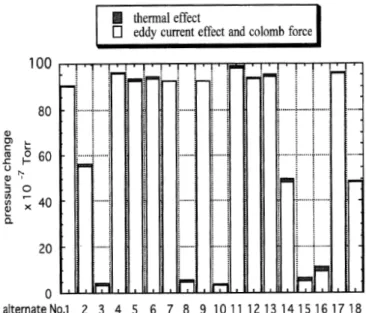
Isogai studied in 1997 some of the most relevant drag sources [47]. According to his work, there are three main sources for error in the measurement of the SRG’s drag: temperature, electrostatic force (or Coulomb force as Isogai refers to it) and eddy currents.

_˙ ω ω total = _˙ ω ω gas + _˙ ω ω eddy currents + _˙ ω ω temperature + _˙ ω ω electrostatic force (3.18)

Temperature error can be troublesome for two reasons: because the temperature is included in the equation of the relative deceleration rate in the gas mean thermal velocity (equation 3.11), but also because it affects the rotor’s dimensions and thus its moment of inertia by thermal expansion although it can generally be controlled by keeping the room’s temperature constant. The electrostatic force is exerted on the center of mass of the rotor and therefore is time-independent. Both these forces are responsible for an offset in the pressure reading but are not too difficult to account for in the final reading. Whereas eddy currents induced by the rotating component of the rotor’s magnetic field in the surrounding parts of the instrument, and by external magnetic fields in the rotor itself, are more strictly tied to the residual drag and thus to the low pressure range limitations of the instrument.

Isogai concluded that the deviation due to eddy currents was up to 10 times bigger than the deviation due to thermal effects temperature. Being the measured residual dragg, shown in figure 3.13, roughly equivalent to a pressure of the order or 10−7_{mbar. Other}

culprits for the residual dragg have been identified, like asymmetries in the magnetic field or imperfections in the rotor, which would result in an unequal moment of inertia.

CHAPTER 3. THE SPINNING ROTOR GAUGE

Figure 3.13: Isogai’s results from 18 independent measurements comparing eddy current plus electrostatic force with thermal effects in the SRG output.

Keith also predicted a gravitational radiation effect as a dragg source based on Birkhoff’s theory of gravitation, with an equivalent pressure of the order of 10−12_mbar.

Although with little certainty, Fremerey’s results agreed with Keith’s predictions [49], but his predictions also met some criticism [50].

On the other hand, there is also a high pressure limit for which the equation 3.11 starts to fail. This happens when the pressure rises above the molecular regime, which for Fremerey’s SRG would start to happen for pressures above 10−2_mbar.

Figure 3.14: Non-linearity curve for higher pressures [51].

However, despite not being linear, the pressure reading can be corrected. Even though

3.3. DRAG SOURCES AND SRG’S LIMITATIONS

the rotor gets very susceptible to thermal errors, due to the increased friction with the gas and the fact that the saturation effect reduces the slop of the plot, which implies an increased measurement uncertainty.

C

H

A

P

T

E

R

4

T

HE

C

HALLENGE OF

L

OW

P

RESSURE

M

EASUREMENT

Vacuum technology operates in a range of over 15 orders of magnitude, as shown in table 4.1. Therefore, there is not one single device that works for every pressure level in vacuum generation or measurement. As a consequence, vacuum pressure is usually divided in several ranges according to the technological requirements to produce or measure it.

Table 4.1: Pressure categories according to the United Kingdom’s National Measurement Institute [52].

Type of Vacuum Pressure Range (Pa)

low vacuum 105_−3×103

medium vacuum 3×103₋₁₀−1

high vacuum 10−1₋₁₀−4

very high vacuum 10−4₋₁₀−7

ultra-high vacuum 10−7₋₁₀−10

extreme ultra-high vacuum <10−10

Note that this is just an example, as there is not one universally accepted method to classify vacuum pressure, and that another source could have a different classification system.

CHAPTER 4. THE CHALLENGE OF LOW PRESSURE MEASUREMENT

Figure 4.1: The pressure range of several manometers [53].

4.1

Direct Pressure Measurement

Direct methods make use of instruments that by definition measure the force the gas exerts in a certain area, i.e. they measure pressure directly. This force can be translated into a mechanical displacement as can be seen in figure 4.2, where a capacitance manometer is represented with a mobile diaphragm. This diaphragm will move according to the pressure difference betweenPX andPR, and by knowing the reference pressurePRit is possible to know the value ofPX.

Figure 4.2: Double-sided capacitance manometer [53].

Other examples of direct instruments are mercury columns, Bourdon or McLeod gauges. Ideally, this would be the only way used to measure pressure, but unfortunately these methods only apply to pressures over 1 mbar (except for the McLeod that can reach

4.2. INDIRECT PRESSURE MEASUREMENT

10−6_{mbar). Measurements under this value become very difficult due to instrument}

limi-tations, since the primary signal is always somewhat related to movement and therefore vulnerable to error sources like vibrations and hysteresis, among others.

4.2

Indirect Pressure Measurement

On the other hand, indirect methods rely on theoretical relationships between pressure and other more easily measurable variables. The knowledge of the various parameters of the system involved in these relationships allow the measured variable to be converted into a pressure reading. Example of these variables are thermal conductivity, ionization probability or coefficient of friction, each of these spanning their own range of instruments and methods.

As an example, thermal conductivity gauges take advantage of the fact that a filament’s resistance change with its temperature, which in this case is used as an indication of the heat transfer between a hot filament and its surroundings. In low pressures, the heat dissipation depends on the pressure since the amount of molecules available to absorb thermal energy is limited. However, different molecules have different heat capacities and consequently the pressure dependence on thermal conductivity has to account for the nature of gas being measured.

This requirement is the most significant disadvantage of these gauges, since the molar mass of the residual gas is of fundamental importance across all indirect methods. Al-though they are usually calibrated for air and can be calibrated for different gases, they can be problematic when dealing with an unknown residual gas.

The spinning rotor gauge is also an indirect method, as it will be further explained.

4.3

Calibration in the Low Pressure Range

Since no instrument operates on the whole spectrum of low pressures, the primary stan-dard used for calibration will depend on the targeted pressure range. Therefore, calibration is carried by two different methods: direct comparison and static or continuous expansion.

Down until 1 mbar, the pressure can be directly measured by mercury columns with low uncertainty. In these circumstances, direct comparison is sufficient for the calibration of an unknown gauge against a standard. It is possible to go even further to 10−6_mbar

with the compression provided by a McLeod gauge.

For lower pressures, static expansion is used to produce a well known pressure. If temperature is kept constant, this expansion can be described by Boyle’s law.

P1V1= P2V2 (4.1)