Multipacket Reception in LTE femtocell networks

(1)

Bruno Alfredo da Silva Branco

Licenciado em Ciˆencias da Engenharia Electrot´ecnica e de Computadores

Multipacket Reception in LTE femtocell

networks

Disserta¸cão apresentada para obten¸cão do Grau de Mestre em Engenharia Electrotécnica e de Computadores, pela Universidade Nova

de Lisboa, Faculdade de Ciˆencias e Tecnologia.

Orientador : Lu´ıs Bernardo, Professor Auxiliar com Agrega¸c˜ao , FCT-UNL

Rui Dinis, Professor Auxiliar com Agrega¸c˜ao, FCT-UNL

J´uri:

Presidente: Prof. Doutor Rodolfo Oliveira Arguente: Prof. Doutor Rui Marinheiro

Vogais: Prof. Doutor Lu´ıs Bernardo Prof. Doutor Rui Dinis

(2)

(3)

i

Multipacket Reception in LTE femtocell networks

Copyright ➞ Bruno Alfredo da Silva Branco, Faculdade de Ciˆencias e Tecnologia, Uni-versidade Nova de Lisboa

(4)

(5)

(6)

(7)

Acknowledgements

I would like to thank my supervisors Prof. Lu´ıs Bernardo and Prof. Rui Dinis, for offering me the opportunity to work in this topic, for his patience and insightful guidance using equipment and other financing provided by FCT/MEC Femtocells(PTDC/EEA-TEL/120666/2010), OPPORTUNISTIC CR(PTDC/EEA-TEL/115981/2009) and ADIN (PTDC/EEI-TEL/2990/2012) projects. My special thanks to all my friends, and office mates for their support at the telecommunication laboratory for their fellowship, great ambiance and their advices to overcome all the difficulties during the thesis realization. Last but not least, my deepest gratitude to my parents and girlfriend, for their love, trust and support.

(8)

(9)

Sum´

ario

A crescente procura por servi¸cos sem fios de banda larga levou ao desenvolvimento e evolu¸cão das tecnologias de rede celular, que prometem ritmos elevados para utilizadores móveis. A 3GPP propôs o LTE (Long Term Evolution) e mais recentemente o LTE-A (LTE advanced). Está prevista a existência de macro esta¸cões base (eNB) e de micro esta¸cões (HeNB), com baixa potência que complementa a cobertura da rede aumentando a densidade de esta¸cões base. Com o inerente aumento da interferência, torna-se essencial uma rece¸cão eficaz. Nesta disserta¸cão é proposta a utiliza¸cão de SC-FDE no downlink de uma rede de femtocells e especialmente a utiliza¸cão da rece¸cão multipacote (MPR) para fornecer servi¸cos de alto débito sem fios. Por outro lado com as crescentes preocupa¸cões ambientais, surgiu o conceito de Green Communications (GC) que visa encontrar solu¸cões para o melhoramento da eficiência energética das redes. Tendo como base os princ´ıpios de GC é proposto um algoritmo para controlar o número de esta¸cões base (principais re-sponsáveis pelo consumo energético das rede sem fios) necessárias fornecer servi¸cos com igual elevada qualidade. Os resultados globais mostram que as tecnologias empregues são uma solu¸cão para obter uma boa rela¸cão desempenho/poupan¸ca energética, indo ao en-contro das exigências (elevadas taxas de dados) e das preocupa¸cões (baixo consumos de energia) da sociedade moderna.

Palavras Chave: Long Term Evolution (LTE), Single Carrier with Frequency

Domain Equalization (SC-FDE), Frequency-Domain Equalization (FDE), Iterative Block-Decision Feedback Equalizer (IB-DFE), femtocell (Home enhanced Node B (HeNB)),Successive Interference Cancellation(SIC),Multipacket Reception (MPR),

Green Communications (GC)

(10)

(11)

Abstract

Driven by the growing demand for high-speed broadband wireless services, LTE technol-ogy has emerged and evolve, promising high data rates to the demanding mobile users. Based on the3rd Generation Partnership Project (3GPP) specifications,Long Term Evo-lution Advanced (LTE-A) telecommunication services predict the existence of macro base stations, Enhanced Node B (eNB) and micro stations HeNB with low power that comple-ments the network’s coverage. This dissertation studies the complementary use of HeNBs (femtocells 3GPP terminology) to provide broadband services. It is essential to main-tain the networks performance with the network densification phenomenon, which brings significant interference problems and consequently more collisions and lost packets. The use of SC-FDE in the downlink of a LTE-A femtocell network - specifically multipacket reception (MPR), with an IB-DFE receiver employing Multipacket Detection (MPD) and SIC techniques is proposed. A new telecommunications concept named GC emerged with the increasing environmental concerns. This dissertation shows the performance results of an iterative MPR and proposes a green association algorithm to change the network layout according to the mobile users demands reducing the Base Station (BS)’s negative contribution to the network total energy consumption. The overall results show that the technologies employed are a solution to achieve a favorable trade-off between performance andEnergy Efficiency (EE), responding to the global demands (high data rates) and con-cerns (low energy consumption and carbon footprint reduction).

Keywords: Long Term Evolution(LTE), Single Carrier with Frequency Domain

Equalization (SC-FDE), Iterative Block-Decision Feedback Equalizer (IB-DFE), Home enhanced Node B (HeNB), Successive Interference Cancellation(SIC),Multipacket Reception(MPR), Green Communications (GC) ,

(12)

(13)

Acronyms

3GPP 3rd Generation Partnership Project

AP Access Point

ARQ Automatic Repeat reQuest

AWGN Additive White Gaussian Noise

BER Bit Error Rate

BS Base Station

CA Closed Access

CDMA Code Division Multiple Access

CoMP Coordinated Multipoint

CP Cyclic Prefix

C-Plane Control Plane

CSG Closed Subscriber Group

DFE Decision Feedback Equalizer

DFT Discrete Fourier Transform

DIM Distributed Interference Management

DL Downlink

EDGE Enhanced Data rates for GSM Evolution

(14)

x ACRONYMS

EE Energy Efficiency

eNB Enhanced Node B

EPC Evolved Packet Core

EPS Evolved Packet System

E-UTRAN Evolved UTRAN

FD Frequency Domain

FDE Frequency-Domain Equalization

FFT Fast Fourier Transform

FFR Fractional Frequency Reuse

GC Green Communications

GSM Global System for Mobile Communications

HA Hybrid Access

HARQ Hybrid Automatic Repeat reQuest

HeNB Home enhanced Node B

HeNB-GW Home eNodeB Gateway

HNet Heterogeneous Network

HSDPA High-Speed Downlink Packet Access

HSPA High Speed Packet Access

HSDPA High-Speed Uplink Packet Access

IA Interference Avoidance

IB-DFE Iterative Block-Decision Feedback Equalizer

(15)

xi

ICI Inter-Carrier Interference

IDFT Inverse Discrete Fourier Transform

IFFT Inverse Fast Fourier Transform

IMT-A International Mobile Telecommunications-Advanced

InH Indoor Hotspot scenario

IPSec Internet Protocol Security

ISI Inter-Symbol Interference

ITU International Telecommunication Union

ITU-R International Telecommunication Union Radiocommunication Sector

LLR Log-Likelihood Ratio

LoS Line-of-Sight propagation

LTE Long Term Evolution

LTE-A Long Term Evolution Advanced

MAI Multi Access Interference

MC Multi-Carrier

MIMO Multiple-Input and Multiple-Output

MME Mobility Management Entity

MMSE Minimum Mean Square Error

MPD Multipacket Detection

MPR Multipacket Reception

NLoS Non-Line-of-Sight propagation

(16)

xii ACRONYMS

OFDM Orthogonal Frequency-Division Multiplexing

OFDMA Orthogonal Frequency-Division Multiple Access

OPEX Operational expenditure

PAPR Peak-to-Average Power Ratio

P-GW Packet-data Network Gateway

PER Packet error rate

PHY Physical layer

PIC Parallel Interference Cancellation

PL Pathloss

QAM Quadrature amplitude modulation

QoS Quality of Service

QPSK Quadrature Phase-Shift Keying

RF Radio Frequency

SAE System Architecture Evolution

SC Single Carrier

SC-FDE Single Carrier with Frequency Domain Equalization

SC-FDMA Single Carrier Frequency-Division Multiple Access

SeGW Security Gateway

S-GW Serving Gateway

SIC Successive Interference Cancellation

SINR Signal-to-Interference-plus-Noise Ratio

(17)

xiii

SON Self-Organizing Network

TD Time Domain

UE User Equipment

UL Uplink

UMa Urban Macro-cell scenario

UMi Urban Micro-cell scenario

UMTS Universal Mobile Telecommunications System

U-Plane User Plane

UTRAN Universal Terrestrial Radio Access Network

(18)

(19)

List of Figures

2.1 LTE Radio Access Network Architecture . . . 7

2.2 OFDM Subcarrier Spectrum . . . 8

2.3 OFDM Block Structure with Cyclic Prefix . . . 8

2.4 Basic OFDM transmitter and receiver block diagram . . . 9

2.5 Transmitter and receiver structure of OFDMA system. . . 9

2.6 Transmitter and receiver structure of SC-FDMA system. . . 10

2.7 OFDMA vs. SC-FDMA . . . 11

2.8 LTE femtocell Radio Access Network Architecture . . . 14

2.9 Two layer network . . . 15

3.1 Basic SC-FDE transmitter and receiver block diagram . . . 22

3.2 SC-FDE receiver structure block diagram . . . 22

3.3 IB-DFE with hard-decisions receiver structure . . . 24

3.4 IB-DFE with soft-decisions receiver structure . . . 26

3.5 IB-DFE with hard and soft decisions performances with QPSK constellation 27 3.6 Suboptimal MPD techniques . . . 28

3.7 Iterative SIC receiver detecting two packets involved in a collision . . . 30

3.8 Propagation Models Indoor Hotspot scenario (InH): Line-of-Sight propa-gation (LoS) and Non-Line-of-Sight propagation (NLoS) Eb/N0 influence . . . 35

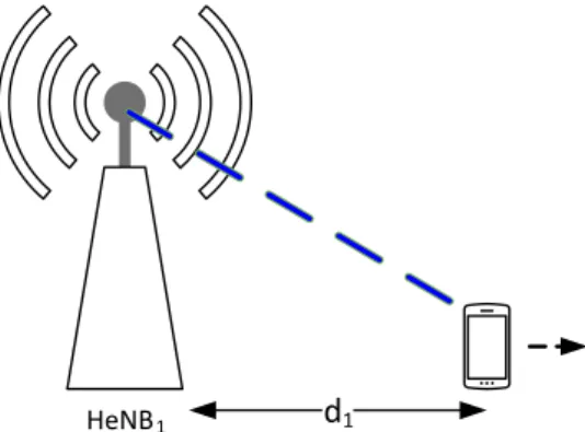
3.9 Simulation scenario used to find HeN B1 range, with P=1 and L=1 . . . 40

3.10 Throughput as a function of distanceHeNB1 - UE . . . 41

3.11 Throughput as a function of Signal-to-Noise Ratio (SNR) . . . 41

3.12 Simple interference simulation scenario used to evaluate receiver perfor-mance, with P=2 and L=1 . . . 42

3.13 Throughput as a function of distanceHeNB1 - UE and HeNB2 - UE . . . . 42

3.14 Throughput as a function of Signal-to-Interference-plus-Noise Ratio (SINR) 43 3.15 Throughput as a function of distanceHeNB1 - UE . . . 43

3.16 HeN B1 and HeN B2 SNR as function of distance . . . 44

3.17 Throughput as a function of distanceHeNB1 - UE . . . 44

3.18 HeN B1 and HeN B2 SNR as function of distance, with L=2 . . . 45

(22)

xviii LIST OF FIGURES

3.19 . . . 45 3.20 Throughput as a function of distance HeNB1 - UE, HeNB2 - UE and

HeNB3 - UE . . . 46

3.21 HeN B1,HeN B2 and HeN B3 SNR as function of distance . . . 46

3.22 Throughput as a function of distance HeNB1 - UE, HeNB2 - UE and

HeNB3 - UE . . . 47

3.23 HeN B1,HeN B2 and HeN B3 SNR as function of distance, with L=2 . . . 47

4.1 Green algorithm procedure . . . 55 4.2 Simulation scenario . . . 55 4.3 Number of active HeNBs as a function of User Equipment (UE) load

(23)

List of Tables

3.1 Simulation parameters . . . 39 4.1 Simulation parameters . . . 56

(24)

(25)

List of Symbols

Bk Receiver feedback coefficients

Eb Average bit energy associated to a given packet transmission

Fk,p Receiver Feed-forward coefficients

H_k,p(l) Channel frequency response from the pth user, during thelth transmission

N0 Power spectral density of the noise

N_k(l) The channel noise during thelth transmission

P Number of transmitting HeNBs

Sk,p Data block transmitted by a userp, in the frequency domain

sk,p Data block transmitted by a userp, in the time domain

T h Throughput

Y_k(l) Received signal, from multiple HeNBs, at the receiver in the frequency

do-main for a given transmissionl τc Cluster delay

Pc Cluster power

λ UE load requirement

(26)

(27)

Chapter 1 Introduction

In recent years, due to the continuous technology development, operators saw a rapid growth of mobile broadband subscribers as well as of their traffic volume demanded, spe-cially due to the introduction of more advanced mobile devices and real time services [1]. As a consequence of this, there is also an increasing demand for high speed data rate services. Under the partnership of the 3GPP, LTE was developed and proposed to sub-scribers to fulfill this ambitious task. LTE evolution, known as LTE-A, was the first to meet the International Mobile Telecommunications-Advanced (IMT-A) requirements for 4G systems, promising among others [2], peak data rates up to 1 Gbit/s. To achieve the desired hight data rates, LTE-A proposed a set of features such as spectrum flexibil-ity, multi-antenna transmission, scheduling and link adaptation, carrier aggregation, relay nodes, Heterogeneous Network (HNet)s andCoordinated Multipoint (CoMP), among oth-ers [3]. LTE radio access exploit rapid variations in channel quality in order to make more efficient use of available radio resources. This is done in both time and frequency do-mains using Orthogonal Frequency-Division Multiplexing (OFDM) and SC-FDE multiple access versions, known as Orthogonal Frequency-Division Multiple Access (OFDMA) and

Single Carrier Frequency-Division Multiple Access (SC-FDMA), in the Downlink (DL) and Uplink (UL) respectively. One of the major concerns is the probable lack of capacity due to the rapid and continuous growth of traffic data demands. The concept of HNet was introduced to face this problem, which briefly consists on adding a second layer to the existing network (macro BSs), dedicated to low power BSs [4]. Seen as the most

(28)

2 CHAPTER 1. INTRODUCTION

cost-efficient solution to both service provider and end user , the femtocell BS (or HeNB in 3GPP) terminology deployment became a reality. Femtocell networks use the same

Physical layer (PHY) technology as macro cellular networks, which means OFDM and SC-FDE multi access versions, serving less users compared to the macro network. Al-though it enhances the overall network performance, the HNet approach also brings new concerns such as the increase of the interference level [4].

1.1 Motivation

According to the requirements, LTE-A is expected to provide higher data rates. Increasing the BSs transmit power seems to be the logical solution. However, it causes higher inter-ference in the network and consequently reduces the network efficiency (performance). To enhance the network performance/efficiency, the decrease of the cell size, reducing the BSs transmit power, seems to be the solution. This reduction is compensated with an increase in the number of deployed BSs in the network. With the emerge of these low power BSs, known as femtocell base stations or HeNB in 3GPPs terminology, the network layout was redesigned, bringing the UEs and the BSs closer to each other. To take advantage of the low power transmissions, an efficient reception becomes essential to enhance HeNBs cover-age range and communication links reliability. In addition, most of the proposed solutions to deal with poor transmission conditions forgot the Energy Efficiency(EE) issue, being typically performance-oriented.

1.2 Objectives and Contributions

(29)

1.3. THESIS STRUCTURE 3

femtocell network - specifically the use of an IB-DFE receiver employing MPD and SIC techniques. The work is divided in two parts: the first part (chapter 3) analyzes the en-hancements achieved with the IB-DFE receiver and MPR technique when multiple HeNBs transmit concurrently. In the second part (chapter 4) it is discussed the appliance of the iterative SIC receiver and MPR technique combined with a switch off technique. The main objective is to achieve the best trade off between performance and energy efficiency, according to the global demands (high data rates) and concerns (low energy consumption and carbon footprint reduction). This work main contributions are :

❼ It shows the IB-DFE receiver employing MPR technique applicability in the downlink of a LTE-A femtocell based network.

❼ The development of a green association algorithm, which achieves a trade-off between energy efficiency and performance, changing the network layout according to the mobile users demands.

1.3 Thesis Structure

Chapter 2 presents the LTE networks key characteristics and features. A brief description of LTE evolutionary process is presented in section 2.1.1. The LTE-A network architecture is depicted in section 2.1.2. The DL and UL multi access schemes adopted are discussed in section 2.1.3. Section 2.1.4 addresses the emerging of small cells. Relevance is given in this thesis to a specific type of small cell named femtocell or HeNB, being explained its concept in section 2.2.1, the fundamental changes that it introduce to the existing network architecture in section 2.2.2 and its modus operandi in terms of access modes and spectrum allocation in sections 2.2.3 and 2.2.4 respectively. Section 2.3 addresses the concept of HNets and discussed the associated interference problems and some possible solutions.

(30)

4 CHAPTER 1. INTRODUCTION

SIC approaches, is explained in detailed in section 3.1.4. In section 3.1.5 it is presented the

Packet error rate (PER) calculation model used in this work. The network interference is characterized in section 3.2. Section 3.3 describes the adopted propagation model, being the detailed explanation of the channel generation process given in section 3.4. Finally, in section 3.5 the performance results regarding to the use of the proposed receiver in the set of chosen simulation scenarios are exhibited and discussed.

(31)

Chapter 2 State of the art

This chapter provides a brief overview of LTE, addressing key topics such as, network architecture, applied multiple access schemes and other relevant issues related to the in-troduction of the small cells (femtocells) approach.

2.1 LTE (Long Term Evolution)

As a consequence of the technological evolution emerged a new concept of mobile users, more demanding and accustomed to access broadband services everywhere.

Mobile broadband, has become a necessity. TheGlobal System for Mobile Communications

(GSM) answered to this trend developing new mobile technologies to achieve high quality of services and better performances, such as higher data rates, larger capacity, greater spectral efficiency, packet switched optimized system and cheaper infrastructure.

LTE was a step beyond 3G and towards the 4G and evolved after Enhanced Data rates for GSM Evolution (EDGE), Universal Mobile Telecommunications System (UMTS),

High Speed Packet Access (HSPA) and HSPA Evolution, to face users increasing demands and ensure 3GPP’s competitive edge over other cellular technologies [5]. The evolution towards LTE began with Release 98 specifying GSM and then continued with Release 99. Release 99 specifies UMTS with Code Division Multiple Access (CDMA) air interface. The technology moved to an all-IP network development in Release 4. UMTS networks development moved to HSPA, introduced in 2002 by Release 5 (High-Speed Downlink Packet Access(HSDPA)) and Release 6 (High-Speed Uplink Packet Access (HSDPA)). The

(32)

6 CHAPTER 2. STATE OF THE ART

improvements in mobile technologies went on by HSPA+, which is described in Release 7.

2.1.1 Evolution to LTE-A

The first version of LTE was completed in March 2009 as part of 3GPP Release 8 and just like the majority of the technologies, it went through an evolutionary process. In order to properly respond to increasing operator and end-user expectations, the LTE radio access technology is continuously evolving. In this evolutionary process, releases 9 and 11 were seen as intermediate releases that introduced multi-cast / broadcast functionality and CoMP transmission and reception of BSs respectively.

Releases 10 and 12 were the major steps in this continuous evolution. The first one commonly referred to as LTE-A [6] introduced carrier aggregation, Multiple-Input and Multiple-Output (MIMO) evolution up to 8×8 and 4×4 in the DL and UL respectively, relay nodes, small cells and HNets [7][8], allowing LTE to meet IMT-A requirements for 4G systems, such as peak data rates up to 1 Gbit/s, as defined by the International Telecommunication Union Radiocommunication Sector (ITU-R)[9].

3GPP’s release 12 targets the increasing demand for mobile broadband services and traffic volumes focusing areas like capacity increase, energy savings, cost efficiency, support for diverse application and traffic types, higher user experience/data rate and small cells [10].

2.1.2 Network Architecture

LTE embraces the evolution of the radio access through theEvolved UTRAN (E-UTRAN), accompanied by the evolution of non-radio aspects termedSystem Architecture Evolution

(SAE), originating the overall architecture termed Evolved Packet System (EPS) [11]. The Evolved Packet Core (EPC), or EPS core network, is a flat, packet switched all-IP network . Its architecture is divided in two planes: Control Plane (C-Plane) and User Plane (U-Plane). EPC consists of functional entities including C-Plane nodes such as

(33)

2.1. LTE (LONG TERM EVOLUTION) 7

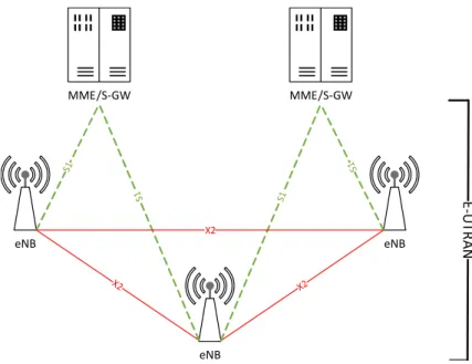
as well as, implement all related radio functions, such as Radio Resource Management, Header compression, security, positioning and connectivity to EPC. The interface X2 enables direct communication between eNBs, supporting mobility, inter-cell interference management andSelf-Organizing Network (SON) functionalities. S1 connects E-UTRAN and EPC, connecting eNBs to MME and S-GW entities .

eNB eNB

eNB

MME/S-GW MME/S-GW

X2

Figure 2.1: LTE Radio Access Network Architecture

2.1.3 Multiple access schemes

The adopted multiple access schemes for DL and UL in LTE are built over OFDM and SC-FDE modulations. This section starts with a brief introduction to OFDM main char-acteristics, being the SC-FDE explained in detail later in chapter 3.

2.1.3.1 Orthogonal Frequency Division Multiplexing (OFDM)

(34)

modu-8 CHAPTER 2. STATE OF THE ART

lation scheme (e.g. Quadrature amplitude modulation (QAM) or Quadrature Phase-Shift Keying (QPSK)) at a much lower rate than the original stream, which combined with the use of an efficient implementation of Discrete Fourier Transform (DFT), named as Fast Fourier Transform (FFT), to simplify and improve the channel equalization [15].

Frequency Overlaping Sub-Carriers

Figure 2.2: OFDM Subcarrier Spectrum

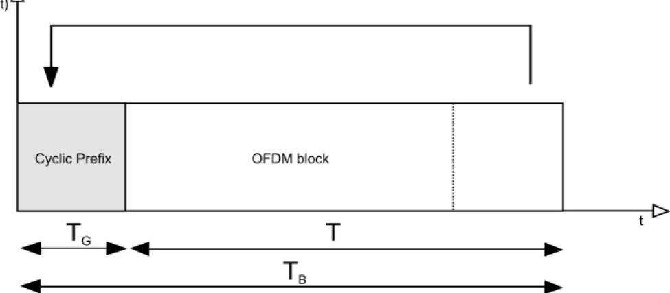
However, communication systems are susceptible to multi-path channel reflections, that leads to delayed copies of the signal and delay spread in transmission, causing Inter-Symbol Interference (ISI). To avoid/reduce ISI, the OFDM based transmitter introduces a guard period, known as theCyclic Prefix (CP), between each transmitted data symbol. The CP is a repetition of the last section of the OFDM symbol that is inserted before to its beginning, that does not carry data and its length is chosen in order to be larger than the expected delay spread of the propagation channel, as depicted bellow in figure 2.3.

OFDM block Cyclic Prefix

T

G

t s(t)

T

B

(35)

2.1. LTE (LONG TERM EVOLUTION) 9

Similar procedures are applied in the reverse order at the receiver side.A simple OFDM block diagram is shown in figure 2.4.

Add CP

Decision

Device

Equalization

Channel

DAC

/RF

Remove CP

IFFT

FFT

_/ADC

RF

Figure 2.4: Basic OFDM transmitter and receiver block diagram

Although OFDM meets the demands for spectrum flexibility and provides cost-efficient solutions for wide-band wireless communications, it has an enormous drawback (especially to UL communication side): the high Peak-to-Average Power Ratio (PAPR), which re-quires linear transmitter circuitry that can be expensive [16].

2.1.3.2 OFDMA in the downlink

OFDMA was chosen to be the transmission scheme in LTE downlink. It is very similar to OFDM, with the main difference that instead of allocating all the available subcarriers, the BS allocates a subset of carriers to each user in order to accommodate multiple trans-missions simultaneously [14]. A block diagram of this multiple access method is depicted in figure 2.5.

Subcarrierz Mapping M-point IDFT AddzCP

/zPS

DAC

/ RF

RemovezCP

M-point

DFT

Subcarrierz De-mappingz/ Equalization

Detection

RF

/ ADC

Figure 2.5: Transmitter and receiver structure of OFDMA system.

(36)

easy to maintain the orthogonality of the subcarriers, whereas in OFDMA, since many users transmit simultaneously, each with their own estimates of the subcarrier frequencies, a frequency offset is inevitable and multiple access interference may occur.

2.1.3.3 SC-FDMA in the uplink

As previously seen in LTE femtocell DL access scheme, the big advantage of OFDMA is its robustness in the presence of multipath signal propagation and its main drawback is the very pronounced envelope fluctuations of the waveform, resulting in a high PAPR in OFDM modulated signals. Signals with a high PAPR require highly linear power amplifiers to avoid excessive inter-modulation distortion. So, to achieve this linearity the amplifiers have to operate with a large back-off from their peak power. Another drawback of OFDMA usage identified for UL transmissions is, the sensitivity to frequency offset (Doppler-Shift). With multiple terminals simultaneous transmissions, different doppler-shifts lead to an orthogonality loss and consequently the introduction of Multi Access Interference (MAI). Since power consumption is one of the main concerns of mobile equipment’s manufactures, this power inefficiency (measured by the ratio of transmitted power to DC power dissipated) induced/caused by OFDMA usage, that increases the cost of the terminal and reduces battery life, led to the choice of the SC-FDMA as the LTE UL transmission technique [17]. SC-FDMA is the multiple access version of SC-FDE, which is similar to OFDM, in that they both perform channel estimation and equalization in the

Frequency Domain (FD). The system model for this access method is depicted in figure 2.6.

N-point

IDFT

M-point IDFT

M-point

DFT

DAC

/RF

AddlCP /l

_PS

RemovelCP

Subcarrierl De-mappingl/ Equalization Subcarrierl Mapping

Detection

N-point

DFT

RF

/ADC

Figure 2.6: Transmitter and receiver structure of SC-FDMA system.

(37)

in-2.1. LTE (LONG TERM EVOLUTION) 11

habit a set of consecutive localized subcarriers achieving frequency-selective gain through channel-dependent scheduling. The main differences between OFDMA and SC-FDMA [18]are:

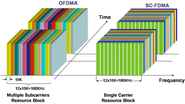
❼ the DFT block placement in the transmitter side, before symbol to subcarrier map-ping, due to the fact that in a Single Carrier (SC) transmission each data symbol is transmitted using the entire allocated bandwidth, while in MC transmission only one subcarrier per data symbol is used.

❼ theInverse Discrete Fourier Transform(IDFT) block placement in the receiver side due to fact that the decision about transmitted bits, contrarily to OFDMA, is done in theTime Domain (TD).

Figure 2.7: OFDMA vs. SC-FDMA

2.1.4 Cell size reduction

(38)

process. This network densification can be achieved with the deployment of complemen-tary low-power BS nodes under the coverage of an existing macro BSs node layer. In such a heterogeneous deployment, low-power nodes bring transmitters and receivers closer to each other providing more spectrally efficient links. Therefore more spatial reuse, higher traffic capacity and end-user throughput (e.g. indoor and outdoor hotspots) is achieved [1], while the macro layer provides wide area coverage. Unlike the high installation and maintenance (infrastructural) cost(s) of macro stations, these low-power nodes constitute a cost-efficient solution to eliminate coverage holes in the network. Types of small cells include femtocells, picocells, metrocells and microcells, broadly increasing in size from femtocells to microcells . Recently, in order to exploit the aforementioned key advan-tages of small-cells in outdoor high-traffic environments, it is emerging a new concept of macro-assisted small cells, termed Phantom Cell [20].

2.2 LTE Femtocells

As mentioned above in section 2.1.4, small cells are seen as the most promising solution to respond to the increasing mobile communications demands. Comparing all employed techniques to increase mobile networks coverage and capacity (e.g. distributed antenna systems and microcells), femtocells seem to be the most cost-efficient solution to both, service provider and end user.

2.2.1 Concept

(39)

2.2. LTE FEMTOCELLS 13

the most relevant aspects in terms of femtocells interference level management, affecting its performance and efficiency (discussion is bellow in sections 2.2.3 and 2.2.4).

Femtocell networks use the same physical layer technology as macro cellular networks, which mean OFDMA in the DL and SC-FDMA in the UL to provide, though limited by the backhaul connection, the desired higher data rates and improvement in terms of

Quality of Service (QoS) to the mobile users [21].

2.2.2 Architecture E-UTRAN

(40)

HeNB SeGW

HeNB-GW

HeNB mgmt system

EPC

S1-MME

S1-U

Figure 2.8: LTE femtocell Radio Access Network Architecture

When present, HeNB-GW serves as a concentrator for the C-Plane, specifically the S1-MME interface and in a manner that mobility issues would not require inter-MME handovers. Besides, it may terminate the U-Plane towards the HeNB and S-GW (S1-U) providing support for U-Plane multiplexing, enhancing systems with limited bandwidth links. The communication between the HeNB and MME/S-GW or HeNB-GW/S-GW is secured by the mandatorySecurity Gateway (SeGW) function. The SeGW establishes and manages all Internet Protocol Security (IPSec) tunnels that each HeNB needs to ensure the integrity of data exchanged with the network. SeGW can be implemented either as a separate physical entity or co-located with an existing entity such as HeNB-GW.

2.2.3 Access modes

Femtocells can support a limited number of users, so it is important to define the set of users that are authorized to use each HeNB resources, in order words to define the access mode. HeNBs can be configured to operate in one of three available distinct modes[23]:

Open Access (OA), Closed Access (CA) andHybrid Access (HA).

❼ OA mode - allows all users to connect to HeNB, usually applied in public places such as airports.

(41)

2.3. TWO TIER NETWORK 15

❼ HA mode - HeNB provides services to its associated CSG members and to non-CSG members, i.e., any UE may access the femtocell (with limited amount of HeNB resources) but preference would be given to those UEs which subscribed to the femtocell. It is usually applied in enterprise environments.

2.2.4 Spectrum allocation

There are two possibilities to deploy femtocells in cellular network spectrum: dedicated channel and shared channel. In dedicated channel deployment, a specific channel is allo-cated for the femtocell network, which is not used by the macrocell; on the other hand, in shared or co-channel deployment the two layers share all channels i.e. the totality of the available spectrum. Due to the high cost and scarcity of spectrum, operators prefer co-channel realization that increases the overall capacity and enhances spectral efficiency, but causes several interference problems that must be dealt [24].

2.3 Two tier network

As previous referred the deployment of small, low power BSs leads to the redesign of the cellular network, dividing it into two main layers, as shown in figure 2.9: macro cellular layer and femto cellular layer. Despite the numerous advantages in terms of capacity, coverage and overall system quality, it also brings some problems/drawbacks and challenges, specifically in terms of interference .

(42)

2.3.1 Interference challenges

To achieve high data rates, the received signal must have a high SINR, depicted in equation 2.1, meaning that each transmitter should not cause significant interference to base station users. It is essential to maintain or enhance network capacity level.

SINR= S

I +N (2.1)

where S, I and N represent the desired signal, the interference signal and the noise, respectively. When I andN have Gaussian distributions, the SINR influence can be seen applying the channel capacity concept to an Additive White Gaussian Noise (AWGN) channel with B Hz bandwidth and SINR, known as the Shannon-Hartley theorem:

C =B×log₂(1 +SINR) (2.2)

The interference impact in the overall network performance depends on the adopted air interface technology, such as the OFDMA applied in the downlink of LTE systems. In order to guarantee the required QoS to eNB users, HeNB available spectrum (bandwidth) is reduced, increasing the odds of occurring co-tier interference at the femtocell network (explained above in section 2.3.1.1). The throughput of the network significantly decreases with all types of interference. Severe interference problems lead to zones where the QoS degrades significantly, termed Dead Zones. Two-Tier network design equally leads to a division in two types of interference: Co-Tier and Cross-Tier interferences.

2.3.1.1 Co-tier interference

(43)

usually is termed as “coverage hole”. This is even more frequent / worrying when HeNBs are working in CA mode (creating wider un-coverage areas). Co-tier interference type is equally divided per communication direction, which means per DL or UL. In the UL side Co-Tier interference is caused by femto UE that act as source of interference to neigh-bor HeNBs. OFDMA femtocells may avoid this type of interference due to the OFDMA division of the spectrum in sub-channels. The BS senses sub-channels conditions. When an UE requires a certain number of sub-channels according to desired QoS, the HeNB allocates sub-channels subject to lower level of interference. The DL Co-Tier interference is caused by a HeNB that acts as source of interference to neighbor femto UEs. This is very common due to the closed distance and dense deployment of HeNBs. Sometimes a simple wall cannot attenuate sufficiently the undesired signals from other BSs. Windows can be a concern too. OFDMA femtocells dynamically sense the air interface and allocate the sub-channels according to sensing results, achieving minimum interference and maxi-mum capacity. 3GPP recommends the use of adaptive power control techniques at HeNBs (especially in CA mode when the serving BS has less power than the interfering one).

2.3.1.2 Cross-tier interference

(44)

is transmitting with high power due to being far away from the macro BS, so the HeNB should allocate different sub-channels in order to avoid interference. In the DL, cross-tier interference can be caused by a HeNB close to a macro UE. If the femto BS is working in CA mode, the area around the HeNB becomes a dead-zone or hole in macro coverage. If HeNB was deployed close to eNB, the femtocell coverage area would be reduced due to the interfering signal from the macro BS. Coverage is guaranteed only very near to the femto BS. In OFDMA the DL interference management is mostly dependent on the sub channels allocation [26].

2.3.1.3 Overcoming challenges

The adoption of an efficient interference management scheme leads to a reduction, miti-gation or in the best scenario elimination of co and cross types of interference and conse-quently to an enhancement in the overall network throughput. Several OFDMA femtocells interference management techniques were mentioned and explained in [27]. They are split in three main sections: Interference Cancellation (IC), Interference Avoidance (IA) and

Distributed Interference Management (DIM).

On this thesis context, more relevance is given to an IC technique named SIC and to an IA technique named spectrum splitting. IC schemes decode desired information, using along channel estimates to cancel the interference. They require the complete knowledge of the interfering signal’s characteristics and an antenna array at the receiver side, making this techniques more suitable to apply in the UL communication and introducing the inherent extra complexity to the BSs. Extensively used in wireless communications, SIC consists in the detection and decoding of one signal per iteration, using the decoded bits from the previous detected signal to cancel it from the combine signal in the next iteration, in order to recover multiple packets . This technique has a complexity and latency proportional to the number of desired signals [28]. For example, when two transmitters share one receiver the common capacity is given by

C = max

B×log₂

1 +S1

N

,

B×log₂

1 +S2

N

(45)

where S1 and S2 are the signals of transmitter 1 and 2 respectively. When employed, SIC capacity gain is observable in [29]:

C=B×log₂

1 +S1+S2

N

. (2.4)

(46)

(47)

Chapter 3 SC-FDE in the downlink

Block transmission schemes combined with frequency domain processing, such as OFDM, proved to be the most effective solution to support high rate transmissions over severe time dispersive channels. Although, present an impressive tradeoff between performance and processing complexity, OFDM has one considerable drawback: the high envelope fluctuation of frequency domain data blocks. This high range of amplitude in the given signal power, measure by the PAPR, appears as a result of high bandwidth demands, due to transmitter power amplifier nonlinearities and leads to the power inefficiency in the Radio Frequency (RF) section of the transmitter. Since the power efficiency became a more relevant issue in mobile communications, a crescent interest in SC modulation methods emerged, which when combined with FDE presents a similar favorable trade-off (performance/low processing complexity) and considerable lower envelope fluctuations than OFDM.

3.1 SC-FDE receiver

In a SC system the signal is transmitted over a single carrier using a conventional mod-ulation scheme such as QAM or QPSK, at a high bit rate. A serious problem to serial data transmissions is the ISI that can be seen as a signal distortion, in which one sym-bol interferes with subsequent symsym-bols, introducing errors in the decision device at the receiver output, making the communication less reliable. This type of interference is usu-ally associated to negative, multi-path propagation or the inherent non-linear frequency

(48)

22 CHAPTER 3. SC-FDE IN THE DOWNLINK

channel response effects. Thus, an efficient equalization, i.e. the compensation of the distortion caused by channel frequency selectivity becomes essential. In SC-FDE systems a nonlinear equalizer is implemented in FD employing FFT and the CP technique (pre-viously explained in section 2.1.3.1), achieving similar performances compared to OFDM with lower complexity, especially on channels with severe delay spread [31].

Insert CP

DAC

_/RF

RF

/ADC

Remove CP

FFT

Channel

Equalization

IFFT

Decision

Device

Figure 3.1: Basic SC-FDE transmitter and receiver block diagram

The low PAPR nature of the SC-FDE systems allows an efficient power amplification with non linear amplifiers [32]. SC-FDE systems present a good performance, being sub-stantially more efficient in terms of power consumption than OFDM systems due to the reduced PAPR. Unlike OFDM systems, in which the decision about the transmitted bits is done in the FD, in SC-FDE systems the decision is performed in the TD, which leads to the inclusion of the IDFT block at the receiver side as shown in figure 3.1.

3.1.1 Linear receiver

DFT

{y

n

}

Decision Device

^ ~

{y

k

}

IDFT

{F

_k

}

{s

k

}

~

{s

_n

}

{s

_n

}

Figure 3.2: SC-FDE receiver structure block diagram

A SC-FDE receiver structure is depicted in fig. 3.2, where the received signal is sampled and its CP removed, resulting in TD samples{yn;n= 0,1, ..., N −1}which after a N-sized

DFT, results in the corresponding FD block {Yk;k= 0,1, ..., N−1}, given by

(49)

3.1. SC-FDE RECEIVER 23

whereHkdenotes the overall channel frequency response for thekth frequency of the block

andNkrepresents channel noise term in frequency-domain. To cope with dispersive

chan-nel effects, FDE is employed and it output, frequency-domain samplesnS˜k;k= 0,1, ..., N −1 o

are given by

˜

Sk =FkYk, (3.2)

where the set of coefficients {Fk;k= 0,1, ..., N −1} denotes the feedfoward FDE

coeffi-cients. To avoid the sub-channels noise enhancement and consequently SNR degradation, that usually occurs when an Zero Forcing (ZF) equalizer is used, it was employed the

Minimum Mean Square Error (MMSE) optimization criteria instead. MMSE minimize both effects of ISI and channel noise enhancement [33]. TheFk applied is

Fk=

H∗

k

α+|Hk|2

, (3.3)

with the noise-dependent term, α, that avoids noise enhancement effects for low values of frequency response Hk, denoted as the inverse of SNR value, more specifically given by

the ratio,

E[|Nk|2]

E[|Sk|2]

= σ 2

N

σ2

S

, (3.4)

whereσ2_N represents the variance of the real and imaginary parts of the channel noise com-ponents{Nk;k= 0,1, ..., N −1} and σ2_S denotes the variance of both real and imaginary

parts of the data samples components{Sk;k= 0,1, ..., N −1}.

3.1.2 Iterative receiver - IB-DFE

(50)

propagation. IB-DFE approach is a promising iterative technique for SC-FDE, proposed in [35], where the feedback and forward operations are both implemented in FD, present-ing low noise enhancement and block reliability on the feedback loop similar to turbo FDE schemes with small error propagation associated [35]. If the estimates of the transmitted block are reliable, the feedback filter can be employed to eliminate the residual ISI. An IB-DFE receiver structure is depicted in figure 3.3,

{Y

k

}

{F_k(i)_}

{s

~n(i)

}

_{s

n

}

^

Decision Device

Delay

+ -^

{s

_k(i-1)

}

DFT

IDFT

DFT

{s

~_k(i)

}

{s

~k(i-1)

}

{B_k(i)_}

{Y

_n

}

Figure 3.3: IB-DFE with hard-decisions receiver structure

where for the ith _{iteration, the DFE output block samples are given by}

˜

Sk

(i)

=F_k(i)Yk−B( i)

k Sˆk

(i−1)

, (3.5)

with

Yk=SkHk+Nk, (3.6)

where nF_k(i);k= 0,1, ..., N−1o and nB(_ki);k= 0,1, ..., N −1o are the feedfoward and feedback coefficients respectively. nSˆk

(i−1)

;k= 0,1, ..., N −1orepresents a DFT of the

es-timated (hard-decision) block of the previous DFE iteration transmitted block{sn;n= 0,1, ..., N −1}.

Both feedfoward (F_k(i)) and feedback (B_k(i)) IB-DFE coefficients, are chosen to maximize themSINR, which is seen as the IB-DFE optimization.

SINR(i) =

γ

(i)

2 E

|Sk|2

E

|ε(_ki)|2

(51)

Considering a hard decision IB-DFE, the optimum B(_ki) and F_k(i), respectively, are

B_k(i)=ρ(i−1)(F_k(i)Hk−γ(i)) (3.8)

and

F_k(i) = κ

(i)_H∗

k

α+ (1−(ρ(i−1)₎2_)|_H

k|2

(3.9)

where κ(i) _{is chosen to assure that the ”mean value of the channel”}

γ(i)= 1

N

N−1

X

k=0

F_k(i)Hk= 1. (3.10)

The α coefficient is given by equation 3.4 and the correlation coefficient from the previ-ous iteration ρ(i−1)_{, which is determinant to ensure a good receiver performance since it} supplies a block-wise reliable measure of the estimates employed in feedback loop. It is defined as

ρ(i−1) = E[ ˆsn (i−1)_s∗

n]

E[|sn|2]

= E[ ˆSk (i−1)

S∗

k]

E[|Sk|2]

, (3.11)

where ˆsn(i−1)represents the data estimates associated to the previous iteration and ˆSk

(i−1)

its associated DFT result. In order to reduce error propagation associated problems hard-decisions per block and overall block reliability are considered in the feedback loop. There-fore, for the first iteration the IB-DFE receiver is simply reduced to a linear FDE.

3.1.3 IB-DFE with soft decisions

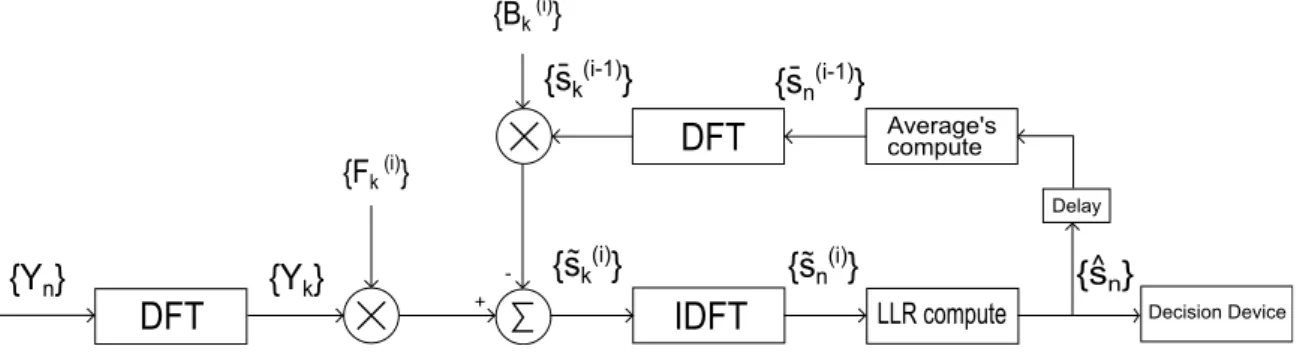
As depicted in figure 3.5, the IB-DFE performance can be improved with the use of “soft decisions”, ¯s(ni), instead of “hard decisions”, ˆs(ni), meaning the use of symbol averages

instead of blockwise averages. So applying the soft estimation, the equation (3.5) can be rewritten as

˜

Sk

(i)

=F_k(i)Yk−B_k(i)S¯k(i−1), (3.12)

in which the soft decision estimates from the previous iteration, ¯Sk(i−1), i.e. the overall

block average of Sk(i−1) at the ‘DFE output’, is given by

¯

Sk(i−1) =ρ(i−1)Sˆk

(i−1)

(52)

where ρ(i−1) _{represents the block wise reliability of the hard decision estimates ˆ}_S

k

(i−1) . LLRFcompute Average's compute +

-{s_k(i-1)_}

-Delay

DecisionFDevice

IDFT

DFT

{Yn} {Yk}

{F_kF(i)_}

{B_kF(i)_}

{s_n(i-1)}

{s~_k(i)_} _{s

n(i)} ~

DFT

{s^n}

Figure 3.4: IB-DFE with soft-decisions receiver structure

The receiver structure for IB-DFE with “soft-decisions” is depicted in figure 3.4, being the used feedforward coefficients (F_k(i)) given by equation 3.9. At the DFE output, the TD samples (˜s(ni)) are de-mapped into the corresponding bits by means of computing the

Log-Likelihood Ratio (LLR) of each bit of the transmitted symbols. Assuming that the transmitted symbols are selected from a QPSK constellation with gray mapping, then

sn = sIn+js

Q

n = ±1±j in which sIn and s Q

n denote the real and imaginary parts of sn,

respectively.

Thus, the LLRs of “in-phase bit” and “quadrature bit”, associated tosn, are

LI(i)

n =

2˜sIn(i)

σ2

i

, (3.14)

and

LQ_n(i)= 2˜s

Q(i)

n

σ2

i

, (3.15)

respectively, with ns˜(ni);n= 0,1, ..., N −1 o

= IDFTnS˜_k(i);k= 0,1, ..., N −1o. The variance σ2 _{is given by}

σ_i2 = 1

2E

|sn−˜s( i)

n |2

≈ 1 2N

N−1

X

n=0

|ˆs(_ni)−s˜(_ni)|2, (3.16)

where ˆsn=±1±j are the hard-decisions associated to ˜sn.

Therefore, the average symbol values conditioned to the DFE outputns¯(ni);n= 0,1, ..., N−1 o

, are

¯

s(_ni)= tanh LI_n(i)

2

+jtanh LQ_n(i)

2

(53)

with ρI n, ρ

Q

n denoting the reliabilities related to in-phase and quadrature bit of the nth

symbol, respectively.

Consequently, the correlation coefficient that will be employed to compute the optimal feedforward coefficients in order to minimize the SINR for a QPSK constellation, is

ρ(i)= 1

2N

N−1

X

n=0

ρIn(i)+ρQn(i)

(3.18)

0 2 4 6 8 10 12 14 16

10−4

10−3 10−2

10−1 100

Eb/N0(dB)

B E R ----/IB-DFE/HD //////IB-DFE/SD //////MFB (+)/1st/iter. (//)/2nd/iter. (//)/3rd/iter. (o)//4th/iter.

Figure 3.5: IB-DFE with hard and soft decisions performances with QPSK constellation

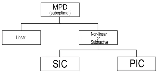
3.1.4 Multipacket Reception

(54)

interference) detection techniques.

Non-linear or Subtractive

SIC

MPD

(suboptimal)

Linear

PIC

Figure 3.6: Suboptimal MPD techniques

The Decorrelating and MMSE are the most popular multiuser linear detectors, in which a linear mapping to the soft output of a conventional detector is applied, in order to reduce the MAI. However, there are fundamental differences between these two linear de-tectors. Whereas the Decorrelating detector (highly analogous to ZF equalizer) attempts to completely eliminate the MAI from all users, applying the inverse correlation matrix at the match filter bank output, the MMSE instead tries to minimize the square of residual noise plus interference applying a modified inverse correlation matrix at the match filter bank output, obtaining better results than the Decorrelating detector which often results in an unacceptable noise enhancement.

Subtractive interference or IC techniques require reliable received signal estimation, mean-ing an accurate description of what was transmitted as well as the channel effects in that transmission. These techniques can be organized in two categories: the use of a parallel

(55)

to the composite received signal. Although PIC presents a lower latency, it usually has a higher level of complexity compared to SIC approach which has a complexity and latency proportional to the number of packets [28].

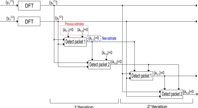
There are several MPD approaches. In this study a MPD technique based on time diversity [32] was considered, in which all transmitters involved in a collision (P), transmit several copies of their packets under slightly modified transmission conditions, in order to allow their separation at the receiver. So, the received content at the UE{Yk;k= 0,1, ..., N−1}

is

Y_k(L)=H_k,P(L)Sk,P+N( L)

k , (3.19)

or the expanded expression

     

Y_k(1)

.. .

Y_k(L)

      =      

H_k,(1)₁ · · · H_k,P(1)

..

. . .. ...

H_k,(L₁) · · · H_k,P(L)

           

Sk,1 .. . Sk,P       +      

N_k(1)

.. .

N_k(L)

      . (3.20)

where L denotes the number of required retransmissions, meaning the temporal diversity order and P represents the number of BSs involved in the transmission.

As aforementioned in section 3.1.2, both feedforward and feedback filters are implemented in FD, being, for each iteration, the first responsible for partially equalizing the interference and the second for the partial removal of the residual interference.

(56)

{an,1}=0

_

{yn(1)}

DFT

Detect packet 1

Previous estimates

New estimate

2nd_iteration

{yn (2)_}

DFT

{yk(1)}

{yk (2)_}

{an,2}=0

_

{a__n,1}=0

{an,2}=0

_

{a__n,2}=0

{a__n,2}=0 {a__n,1}=0

1st_iteration

Detect packet 2

Detect packet 1

Figure 3.7: Iterative SIC receiver detecting two packets involved in a collision

When detecting a packet its residual ISI is removed, as well as the residual interference from other packets. The receiver is composed by NP FD feedfoward filters, one for each retransmissionl and NP FD feedback filters one for each packetp. This SIC receiver uses the average values associated to a given packet ¯sn,p, conditioned to DFE output given by

˜

Sk,p=

N P X

l=1

F_k,p(l)Y_k(l)−

P X

p′₌₁

B_k,p(p′)S¯k,p′ (3.21)

where the average values ¯Sk,p′ are computed as previously explained in section 3.1.3, so

the optimum feedfoward that minimize SINR for a given packet and iteration are

F_k,p(l) = ˘

F_k,p(l) γp

(3.22)

with

γp =

1

N

N−1

X k=0 N P X l=1 ˘

(57)

being ˘F_k,p(l) computed from

(1−ρ2_p)H_k,p(l)∗

N P X

l′₌₁

˘

F_k,p(l)F˘_k,p(l)+X

p′₆₌_p

(1−ρ′_p2)H_k,p(l)∗′

N P X

l′₌₁

˘

F_k,p(l)H_k,p(l′)′∗+αF˘

(l)

k,p=H

(l)∗

k,p, l= 1, ..., N P,

(3.24) where the correlation coefficientρis defined as in equation 3.18 and reproduced in equation 3.25 for a given user p and iterationi.

ρ(_pi)= 1 2N

N−1

X n=0 ℜ n ¯

s(_n,pi)o + ℑ n ¯

s(_n,pi)o

. (3.25)

So, the feedback coefficients are given by

B_k,p(p′) =

N P X

l=1

F_k,p(l)H_k,p(l)′−δp,p′, (3.26)

with δp,p′ =

  

 

1 if p6=p′

0 if p=p′.

3.1.5 IB-DFE receiver performance

The IB-DFE receiver decodes the HeNB’s L transmissions up to Niter iterations. The

estimated data symbol ˜S_k,p(i), for a given iteration iand HeNBp is

˜

S_k,p(i) =F_k,p(i)TYk−B( i)T

k,p S¯

(i−1)

k (3.27)

where F_k,p(i,l)T and B_k,p(i,l)T with l = 1,2, ..., L are the feedfoward and feedback coefficients respectively. ¯S_k,p(i−1) with p = 1, .., P are the soft decision estimates from the previous iteration for all HeNBs. ¯S_k,p(i−1) can be related to symbols hard decisions, ˆS_k,p(i−1) as

¯

S_k,p(i−1) ≃P(i−1)Sˆ_k,p(i−1) (3.28)

ˆ

S_k,p(i−1)=P(i−1)∆k (3.29)

whereP(i−1)₌_diag₍_ρ(i−1)

1 , ..., ρ

(i−1)

P ) are the correlation coefficients and ∆k= [∆

(1)

k , ...,∆

(P)

k ]T

(58)

for a given HeNB pis

ρ(i−1)= 1

2N

N−1

X n=0 ρ I n,p

(i−1)

+ ρ Q n,p

(i−1)

. (3.30)

For the first iteration (i = 1), ¯S_k,p(i−1) is a null vector and P(i−1) _{is a null matrix. As} aforementioned, theF_k,p(i,l)and feedbackB_k,p(i) coefficients are selected to minimize the SINR, for a given packet and a given iteration. This optimization problem can be written as the minimization of MMSE, E

Sk,p−

˜

S_k,p(i)

2

, of Sk,p :

E

F_k,p(i)T(HT

kSk+Nk)

−

B_k,p(i)TP(i−1)₍_P(i−1)_S

k+ ∆k) + ΓpSk 2 . (3.31)

To obtain the optimal coefficients,F_k,p(i) andB(_k,pi), under the MMSE criterion , the gradient of the Lagrange function is applied to equation 3.31:

∇J =∇

E

Sk,p−S˜

(i)

k,p

2

+ (γ_p(i)−1)λ(_pi)

(3.32)

conditioned to

γ_p(i)−1 = 1

N

N−1

X

k=0

L X

l=1

F_k,p(i,l)H_k,p(l) −1. (3.33)

The following set of equations

            

∇_F(i)

k,p

J = 0

∇

B(_k,pi)J = 0

∇_λ(i)

p J = 0

(3.34)

were verified when

γ_p(i) = 1. (3.35)

For a single HeNB ptransmitting data, i.e. without collisions, results

γ_p(i) = 1, (3.36)

B_k,p(i) =

L X

l=1

F_k,p(i,l)H_k,p(l) −γ(i)

(59)

F_k,p(i,l)= γ (i)

p H(l)

∗ k,p σ2 N σ2 S L P l=1 H

(l)

k,p

2. (3.38)

σ2_p(i) = 1

N2

N−1

X k=0 E S˜

(i)

k,p−Sk,p

2

. (3.39)

Assuming the Gaussian behavior of the overall interference Nk that affects the symbol

estimation, in accordance to [37], the symbol error probabilityPsfor a QPSK constellation

is denoted by

Ps≃2Pe

ηk> p

Eb

= 2Pe

ηk σp > s Eb σ2 p !

= 2Q

s Eb σ2 p ! , (3.40)

where Q(x) is the well known Gaussian error function. Assuming that Eb = 1, the Bit

Error Rate (BER) for a given HeNBpis

BER_p(i)≃Q 1

σp(i) !

. (3.41)

For an uncoded system with independent and isolated errors, the PER for a fixed packet size of M bits is

P ER(_pi)≃1−1−BER(_pi)M. (3.42)

PER values are used to compute the HeNBs associated throughput at the receiver, denoted as

T h= W(1−P ER)

L , (3.43)

(60)

3.2 Femtocell interference characterization

This dissertation analyses the performance of the IB-DFE receiver when multiple femto BSs (HeNBs) transmit. A SC-FDE downlink channel is considered. For the receiver algorithm [37], using the receiver performance model presented in the subsection above can be used to characterize the system performance. The PER and BER are defined as a function, < BER;P ER >= f(Hk;Eb/N0) , which depends on the channel and on the transmission power. The energy per bit to noise power spectral density ratio,

Eb/N0, is an important parameter in digital communication or data transmission. It is a normalized SNR measure. Eb/N0 is equal to the SNR divided by the link spectral efficiency in (bit/s)/Hz, where the bits in this context are the transmitted data bits. The SINR is normally used to characterize the interference caused by others transmissions in the reception at the UE of the desired signal. It is defined as

SINR= PR

Pnoise+PI

(3.44)

where PR and PI denote the received power of the, desired signal from HeNB1 and the signal from the P-1 interfering HeNBs. The received signal strength goes down as the

Pathloss (PL) (explained in section 3.3) increases with the distance from the serving HeNB. The reception power is calculated using

PT −PL, (3.45)

where PT denotes the HeNB transmit power and PL represents the path loss value

(61)

3.3. PROPAGATION MODEL 35

3.3 Propagation Model

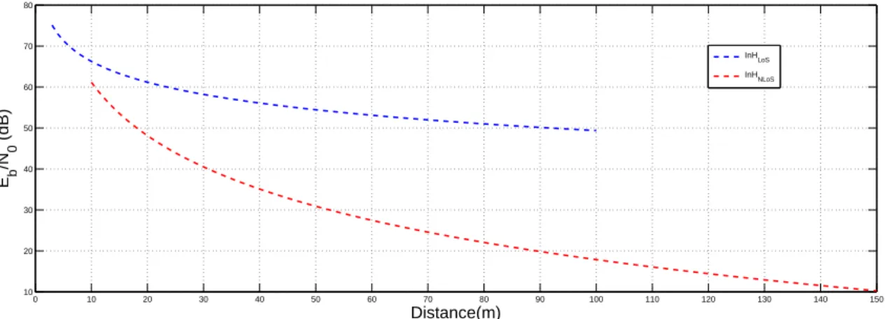
The receiver performance is strongly influenced by the characteristics of the channel. These characteristics depend upon the distance between the two antennas (transmitter and receiver) and the signal path(s). To support the development of 4G, ITU-R has adopted a number of models [38] to characterize different transmission scenarios, including:

Urban Macro-cell scenario (UMa), Urban Micro-cell scenario (UMi) and Indoor Hotspot scenario(InH). For distances between 3 and 150 meters, common in femtocells hotspot, the InH was chosen. The propagation condition, LoS or NLoS, is assigned based on the physical distance (UE - HeNB) and the associated PL is computed as despited in equation 3.46, for each HeNB - UE communication link.

PL

  

 

LoS = 16.9×log10(d) + 32.8 + 20×log10(fc) if d <10

NLoS = 43.3×log10(d) + 11.5 + 20×log10(fc) if d≥10

, (3.46)

where d represents the distance between the pth _{HeNB and the UE given in} _m _and _f c

denotes the HeNB carrier frequency given in GHz. The effect of both pathloss models adopted in terms of Eb/N0(dB)=PT −P L−Pnoise, is depicted in figure(3.8). NLoS and

LoS are valid between 3 and 100 m and 10 and 150 m respectively, whereEb/N0 from LoS is higher than from NLoS channels, for distances above 18 m.

0 10 20 30 40 50 60 70 80 90 100 110 120 130 140 150

10 20 30 40 50 60 70 80

Distance(m)

E b

/N

0

(dB)

InHLoS

InHNLoS

(62)

3.4 Channel coefficients generation

In general, the received signal can be obtained by convolving (in TD) or multiplying (in FD) the transmitted signal with the impulse response of the channel. Therefore, the received signal is:

Yk=HkSk+Nk, (3.47)

where Hk and Nk are the FD channel response and the noise respectively. The Hk

co-efficient for a transmitter and a receiver is defined by a set of signal paths or rays, each with a distinct delay and attenuation, characterized by the tap delay or clustered delay line model :



    

P₍₁₎ τ₍₁₎

.. . ...

P₍C) τ(C)



    

(3.48)

where C denotes the considered number of clusters. A cluster is characterized as a prop-agation path diffused in space, either or both in delay and angle domains [38] or simply as a set of rays. Each cluster delay and power, represented by τ₍c) and P(c) respectively, are computed as follows.

3.4.1 Cluster delay generation

Depending if the propagation condition assigned was LoS or NLoS, the set of delays τ₍_c₎

are generated using a uniform distribution as followed, where rτ is the delay distribution

proportionality factor, στ is the delay spread andXc ∼Uni(0,1).

τ_c′ =−rτστln(Xc) (3.49)

Then the delays are normalized (by subtracting the minimum delay) and sorted in de-scending order.

τc=sort(τ

′

c−min(τ

′

(63)

3.4. CHANNEL COEFFICIENTS GENERATION 37

In the case of a LoS path, an additional scaling was done to compensate peak addition to delay spread,

τ_cLoS = τc

D, (3.51)

where Dis the Ricean K-factor dependent, scaling constant given by:

D= 0.7705−0.0433K+ 0.0002K2+ 0.000017K3 (3.52)

3.4.2 Cluster power generation

Each cluster power or attenuation, P′

(c) is computed based on the above explained delay generation. P′

(c) has an exponential distribution [38],

P₍′_c₎=exp(−τc

rτ−1

rτστ

).10

−Z₍_c₎

10 , (3.53)

where Z₍c)∼N(0, ζ2) denotes the shadowing term. Then P′

(c) is normalized,

Pc =

P_c′

C P c=1 P′ c , (3.54)

and in the case of LoS path, an additional specular component is added to the first cluster

P1,LoS =

KR

KR+ 1

, (3.55)

so the LoS cluster powers are

Pc,LoS =

1

KR+ 1

P_c′

C P

c=1

P′

c

+δ(c−1)P1,LoS, (3.56)

In this performance model it is assumed that theHeNB1transmits duringLslots and that the otherP−1 also transmit simultaneously during theLslots. Let{sn,1;n= 0,1, ..., N −1} denote the data block from the HeN B1 and {sn,p;n= 0,1, ..., N−1} from the HeN Bp

and their corresponding frequency domain blocks, after applied an size-N DFT operation,

(64)

number of data symbols.

The received content at theUE,{Yk;k= 0,1, ..., N −1}, depends on theLchannel

realiza-tions of the P HeNBs (Hk,p;p= 1, ..., P), P HeNBs transmitted signals (Sk,p;p= 1, ..., P)

and associated channel’s noise (Nk), and is given by equations 3.19 and 3.20 reproduced

bellow by convenience.

Y_k(l)=H_k,(l)₁Sk,1+· · ·+Hk,P(l) Sk,P+N( l)

k , (3.57)

or the expanded expression

     

Y_k(1)

.. .

Y_k(L)

      =      

H_k,(1)₁ · · · H_k,P(1)

..

. . .. ...

H_k,(L₁) · · · H_k,P(L)

           

Sk,1 .. . Sk,P       +      

N_k(1)

.. .

N_k(L)

      , (3.58)

where Hk denotes the channel frequency response computed from tap delay values (3.48)

and Nk denotes the corresponding channel noise.

3.4.3 Channel modeling

The channel model is influenced by the interference pattern, modeled by ITU-R [38], and by the spatial distribution of the HeNBs and the UEs. The two contributions are modeled in theHk,l matrix coefficients. The signal attenuation associated to the transmission from

a HeNB and the UE is defined by the PL, which depends of the distance and the channel model and can be calculated using [38] (see equation 3.46),

ξ(l, p) = 10−PL20(p). (3.59)

The coefficients that form theH matrix are calculated assuming a reference transmission power, so the equivalent PL is defined asPL=PTref−PR, wherePT =PR+P L. Finally,

the coefficients for theL channel realizations of the pth _{HeNB are given by}

(65)

3.5. PERFORMANCE RESULTS 39

So the received content at the UE, given by equation 3.57, can be rewritten as

Y_k(l)=ξ(l,1)H_k,(l)₁Sk,1+

P−1

X

p=1

ξ(l, p)H_k,p(l)Sk,p+N_k(l), (3.61)

for a scenario with P-1 interfering HeNBs.

The PER values for the iterative receiver can be calculated extending the models intro-duced in sections 3.1.3 and 3.1.4. The linear one is a special case of the IB-DFE, where the number of iterations (Niter) is equal to 1.

3.5 Performance results

This section presents a set of performance results for the proposed IB-DFE receiver in time-varying channels. It was considered a SC-FDE modulation, with FFT-block of N=256 data symbols and a CP of 32 symbols, longer than overall delay spread of the channel. The simulations were performed in MATLAB➤ following ITU-R M.2135 simulation guideline using the key simulation parameters summarized in Table 3.1.

HeNB transmit power 21 dBm

Bandwidth 20 MHz

Minimum distance (d) between UE serving HeNB 3 m

Carrier frequency (fc) 3.6 GHz

Thermal noise level -174 dBm/Hz

Channel model/PL ITU-R M.2135

InH : LoS orN LoS

Table 3.1: Simulation parameters

Multipacket Reception in LTE femtocell networks

Bruno Alfredo da Silva Branco