Orientador: Professor Doutor Hugo Manuel Brito Águas, Professor Associado, FCT-UNL Co-orientador: Professor Doutor Rui Igreja, Professor Auxiliar, FCT-UNL

(1)

Development of microfluidic droplet generator 1

Francisco Bernardo Gomes Filipe de Matos

Licenciado em Ciências de Engenharia de Micro e Nanotecnologias

Development of microfluidic droplet generator

Dissertação para obtenção do Grau de Mestre em Engenharia de Micro e Nanotecnologias

Orientador: Professor Doutor Hugo Manuel Brito Águas,

Professor Associado, FCT-UNL

Co-orientador: Professor Doutor Rui Igreja,

Professor Auxiliar, FCT-UNL

Júri:

Presidente: Professou Doutor Luís Pereira Arguente: Professora Doutora Joana Pinto Vogal: Professor Doutor Hugo Brito Águas

(2)

(3)

Development of microfluidic droplet generator iii

Development of a microfluidics droplet generator

(4)

(5)

Development of microfluidic droplet generator v

“The most merciful thing in the world, I think, is the inability of the human mind to correlate all its contents... someday the piecing together of dissociated knowledge will open up such terrifying vistas

of reality, and of our frightful position therein, that we shall either go mad from the revelation or flee

from the light into the peace and safety of a new Dark Age.”

(6)

(7)

Development of microfluidic droplet generator vii

Acknowledgement

Com o término deste documento chega ao fim toda uma fase de uma vida, que só foi possível devido ao apoio e paciência de todas as pessoas que tiveram de lidar com a minha pessoa ao longo destes anos. A vaga inicial de agradecimentos é dedicada á instituição que me acolheu e deu oportunidade de crescer como estudante e como ser humano, a Faculdade de Ciências e Tecnologia da Universidade Nova de Lisboa, em particular ao ramo da faculdade em que fiquei inserido, o Departamento de Ciências dos Materiais.

Reconhecimento especial para o professor Rodrigo Martins e para a professora Elvira Fortunato que me permitiram realizar a minha tese numa instituição tão privilegiada como o CENIMAT e pela oportunidade de formar no curso de Engenharia de Micro e Nanotecnologias.

Ao meu orientador, professor Hugo Águas, um grande Obrigado pela ajuda e paciência durante estes meses de desenvolvimento deste trabalho. Um agradecimento também ao meu coorientador, professor Rui Igreja, e a toda a equipa do CENIMAT pela ajuda dada sempre de boa vontade e em bom espírito.

Longe de casa e sem conhecer ninguém devo o minha continua sanidade e bom humor à família que se criou no Monte da Caparica, Inês, Xana, Jolu, David, Alex e Crespo, a todos eles um grande abraço e que venham muitos mais anos unidos. Para além da família do Monte devo também um obrigado a colegas cuja paciência para me aturar durante 6 anos faz inveja a um santo, Emma, Bela, Cátia, Farto, Sara, Viorel, Saraiva, Tó, e a muitos mais de quem em possa ter esquecido.

Houve muitos fins-de-semana que fui impedido de voltar a Vila Real, por essa razão devo um pedido de desculpas com a mais pura das intenções, a todos os meus compadres transmontanos: Ricardo, Bruno, Renato, Rafa, Duarte, Vasco, João, Pedro, Jorge, Daniel, Rodrigo, Toni e Fred.

(8)

(9)

Development of microfluidic droplet generator ix

Abstract

The need for mass scale testing in areas such as microbiology and chemistry requires faster processing times, multiplexing capability, and reduced reagent requirements. To achieve this, the volumes processed must be reduced. This work intends to produce a microfluidic chip capable of producing increasingly smaller droplets that serve as testing vessels, by taking advantage of the dynamics of two immiscible fluids. The purpose of the present chip is to be used in the future in a digital Polymerised Chain Reaction (dPCR) for DNA amplification and detection.

The microfluidic device was first simulated using COMSOL Multiphysics to understand the different behaviours of the droplet generator junctions. Glass sealed devices were produced using soft-lithography, composed of two different parts, a glass substrate and a top PDMS slab fabricated by photolithography of a SU-8 mould on a Si wafer that was used to mould the PDMS.

Devices were tested with two immiscible fluids, which were injected at a constant flow rate into two inlets that lead to the junction were the droplets were formed. We were able to obtain droplets as small as 1 nL in devices with a channel size of 50 µm. We concluded that reducing the entry section to the main channel until the junction point, will decrease droplet size keeping the same size of the channels after the junction. Faster droplet generation rate was also obtained, using side channels width smaller (50 µm) than the main channel (100 µm).

(10)

(11)

Development of microfluidic droplet generator xi

Resumo

A necessidade de testes em grande escala em áreas como microbiologia e química requer tempos de processamento mais rápidos, capacidade de multiplexing e redução de volumes de reagentes. Para

conseguir isso, os volumes processados devem ser reduzidos. Este trabalho pretende produzir um chip de microfluídica capaz de produzir gotículas cada vez menores, que servem como vasos de teste, aproveitando a dinâmica de dois fluidos imiscíveis. O objetivo do presente chip é para ser usado no futuro em uma reação em cadeia polimerizada digital (dPCR) para amplificação e deteção de DNA.

O dispositivo de microfluídica foi simulado inicialmente usando o COMSOL Multiphysics para entender os diferentes comportamentos das junções do gerador de gotículas. Dispositivos selados em vidro foram produzidos usando soft-litografia, que é composta de duas partes diferentes, um substrato de vidro e um pedaço de PDMS superior fabricado por fotolitografia de um molde SU-8 numa pastilha de Si que foi usada para moldar o PDMS.

Os dispositivos foram testados com os dois fluidos imiscíveis, que foram injetados a um fluxo constante em duas entradas que levam à junção onde as gotículas foram formadas. Conseguimos obter gotículas tão pequenas quanto 1 nL em dispositivos com tamanho de canal de 50 µm. Concluímos que a redução da seção de entrada para o canal principal até o ponto de junção diminuirá o tamanho das gotas mantendo o mesmo tamanho dos canais após a junção. Taxa de geração de gotas mais rápida também foi obtida, usando canais laterais com largura menor (50 µm) do que o canal principal (100 µm).

Palavras-chave: Junção-X; Junção-T; Junção-Y; Dripping; Jetting; Squeezing; COMSOL; SU-8;

(12)

(13)

Development of microfluidic droplet generator xiii

Abbreviations and Acronyms

dPCR Digital Polymerase Chain Reaction

DNA Deoxyribonucleic acid

PDMS Polydimethylsiloxane

W/O Water-in-Oil

O/W Oil-in-Water

UI User Interface

IPA Isopropyl Alcohol

USB Universal Serial Bus

(14)

(15)

Development of microfluidic droplet generator xv

Symbols

ρ Density

u Flow speed

γ Surface tension

L Characteristic dimension Le Entrance Length Re Reynolds Number Ca Capillary Number µ Dynamic Viscosity g Gravity constant

(16)

(17)

Development of microfluidic droplet generator xvii

List of Figures

Figure 1 dPCR microfluidic chip layout, with separate zones for the different temperatures required for a successful PCR. Adapted from [5]. ... 1

Figure 2 Schematic of three types of junctions with their respective functioning regimes. Adapted from [11] ... 3

Figure 3 a) Alternating X-Junction; b) regular X-Junction Adapted from [13]. ... 4 Figure 4 Example of a Y-Junction. Adapted From [13] ... 5 Figure 5 Generic Flow-Focusing device. In these add-ons the junction is before the point of smaller width ... 6

Figure 6 Schematic of a soft-lithography process. a) Starting Si wafer; b) Deposition of a thin film of SU-8; c) SU-8 exposure through the designed mask; d) Developing of the SU-8 leaving the mould; e) Casting of PDMS on top of the SU-8 mould; f) Curing of PDMS at 70 ºC; g) Peel off of the PDMS from the mould; h) Sealing of the PDMS device to a piece of glass. ... 7

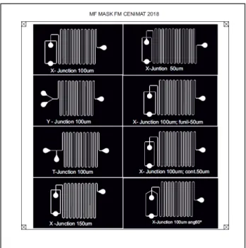
Figure 7- Negative mask used for SU-8 mould production. X-Junction 100 µm, X- junction with all the channels 100 µm wide; X-Junction 50um, X- junction with all channels 50 µm wide; Y-Juntion 100 µm, Y junction with all channels 100 µm wide; X-Junction 100 µm funil-50 µm, X -junction with a 50 µm wide and 30 µm long channel after the junction, then opening up to a 100 µm wide channel like the pre-junction channels; T-Junction 100 µm, T-junction with all channels 100µm wide; X-junction 100 µm cont.50 µm, the side channels (continuous phase channel) are 50 µm wide but the dispersed phase and main channel is 100 µm wide; Junction 150 µm, junction with all channels 150 µm wide; X-Junction 100 µm ang60°, X junction with all channels 100 µm wide but with a 60° angle between the main channel and each of the continuous phase channels. A larger and more detailed version can be seen in appendix B ... 8

Figure 8 Film capture set-up; A) Two 10 ml syringes one holding water with blue food colouring and other containing the Silicone oil 50 cSt ;B)Injector pump, sustains a continuous pressure on both syringes ensuring a constant flow rate injected into the device inlet ;C) USB microscope used to record videos of the working device on the laptop; D) Optical microscope used to find clogs along the channels, discriminating functioning and obstructed device ... 9

(20)

Figure 12 Complete droplet generator, Y-Junction in this case. An individual photo of all droplet generator chips can be found in Appendix D. ... 12

Figure 13 Frame of simulated X-Junction 100 µm wide, at 2.0 µL/min. The water is presented in red and the oil in blue, the interface is presented in yellow because the chosen mesh is a coarser grid in order to speed up simulations. This means that the interface is presented as a mixture of water and oil, instead of a clear and abrupt phase difference. ... 13

Figure 14 Frame of simulated T-Junction 100 µm wide, at 2.0 µL/min. The water is presented in red and the oil in blue, the interface is presented in yellow because the chosen mesh is coarser to speed up simulations. ... 13

Figure 15 Assumed front views of the droplets a) Maximum channel occupation possible corresponding to maximum possible volume on any channel; b) Minimum occupation of the main channel for the 50µm wide channel; c) Minimum occupation of the main channel for the 150µm wide channel; d) Minimum occupation of the main channel for the 100µm wide channel; ... 14

Figure 16 Range of droplet volumes for droplet for the X-Junction 100 µm wide, in these graphs the error bars represent the maximum and minimum possible volumes that were calculated and the point represents the average volume of those calculations. ... 15

Figure 17 Frames of the captured film of the 100 µm wide X- junction at different flow rates, from left to right, top to bottom 0.5 µl/min to 3.0 µl/min. The first given scale applies to the first two panels (0.5 ul/min and 1.0 ul/min) and the second applies to the remaining panels. ... 16

Figure 18 Range of droplet volumes for the X-Junction 50 µm wide ... 16 Figure 19 Frames of the captured film of the 50 µm wide X- junction at different flow rates, from left to right, top to bottom 0.5 µl/min to 3.0 µl/min ... 17

Figure 20 Range of droplet volumes for droplet for the Y-Junction 100 µm wide ... 18 Figure 21 Frames of the captured film of the 100 µm wide Y- junction at different flow rates, from left to right, top to bottom 0.5 µl/min to 3.0 µl/min ... 18

Figure 22 Range of droplet volumes for droplet for the X-Junction 100 µm wide with side channels 50 µm wide. ... 19

Figure 23 Frames of the captured film of the 100 µm wide X- junction with 50 µm wide side channels at different flow rates, from left to right, top to bottom 0.5 µl/min to 3.0 µl/min. ... 20

Figure 24 Range of droplet volumes for droplet for the X-Junction 100 µm wide with a flow focusing device 50 µm wide ... 20

(21)

Figure 27 Frames of the captured film of the 100 µm wide X- junction with side channels joining at a 60º angle to the dispersed phase channel at different flow rates, from left to right, top to bottom 0.5

µl/min to 3.0 µl/min. ... 23

Figure 28 Range of droplet volumes for droplet for the X-Junction 150 µm wide ... 23

Figure 29 Frames of the captured film of the 150 µm wide X- junction at different flow rates, from left to right, top to bottom 0.5 µl/min to 3.0 µl/min. ... 24

Figure 30 Range of droplet volumes for droplet for the T-Junction 100 µm wide ... 25

Figure 31 Frames of the captured film of the 100 µm wide T- junction at different flow rates, from left to right, top to bottom 0.5 ul/min to 3.0 ul/min ... 25

Figure 32 All of the volume graphs combined, as can be seen the Y100 junction is completely outside the 10 nL goal, marked by the dashed line. ... 26

Figure 33 Larger and more detailed version of figure 4 ... 32

Figure 34 X100 junction PDMS chip. ... 35

Figure 35 X50 junction PDMS chip ... 36

Figure 36 Y100 junction PDMS chip ... 36

Figure 37 X100-cont50 junction PDMS chip. ... 36

Figure 38 X100.fun50 junction PDMS chip ... 37

Figure 39 X100-60º junction PDMS chip. ... 37

Figure 40 X150 junction PDMS chip ... 38

Figure 41 T100 junction PDMS chip ... 38

(22)

(23)

Development of microfluidic droplet generator xxiii

List of Tables

Table 1 Dimensionless number that can describe a microfluidic system and their meaning. Adapted from [5]. ... 2

Table 2 Density and Dynamic viscosity for water and silicone oil 50 cSt at 25 ºC [15] required by COMSOL. The water values are automatically filled by the software... 10

Table 3 Combined observed regimes for each junction; D – Dripping; D* – Classified as Dripping but resembles other regime more closely, namely squeezing; S – Squeezing; J – Jetting. ... 26

Table 4 Estimated volumes for the 100µm wide X-Junction ... 31 Table 5 Estimated volumes for the 50µm wide X-Junction ... 31 Table 6 Estimated volumes for 100µm wide Y-Junction ... 31 Table 7 Estimated volumes for X-Junction with 100 µm of width in the main channel and 50 µm of width in side channels ... 31

Table 8 Estimated volumes for the 100µm wide X-Junction with a flow-focusing funnel 50µm wide after the junction point ... 31

Table 9 Estimated volumes for the 100µm wide X-Junction with side channels at a 60º angle with the main channel ... 31

(24)

(25)

Development of microfluidic droplet generator xxv

Motivation and Objectives

With the development of increasingly smaller and more efficient technologies, a question regarding what other areas of scientific knowledge would benefit from a reduction in size of their essential components must be considered [1]. As such, one of the main areas that could benefit from this reduction in size is the study of Biology. Since an essential component to life as we know is water, its separation in small volume droplets in the nL range and the study of individual components of life inside those droplets can be a step forward to advance this field of science. The advantage of working with smaller droplets is the ability of limiting the volume to the reaction vessels (from millilitres to nanolitres), thus reducing the reagents quantity, as well as their costs and reaction time (from minutes or hours to seconds) [2].

(26)

(27)

1. Introduction

1.1 Digital Polymerised Chain Reaction

Digital Polymerase Chain Reaction is an amplification technique based on the division of a sample containing DNA into volumes, where the probability of finding more than one molecule of the target DNA sequence is very low [3]. This technique is particularly suited for very low concentrations of target DNA, which is the case for free circulating DNA from cancer cells present in blood or urine. The digital in dPCR comes from the result in each droplet, using a droplet-based fluorescence signal counting, in which different fluorescence intensities can be represented in binary 1 for a positive detection and 0 for a non-detection[4].

This technique is divided in three temperature dependent steps. The first step aims to denature the DNA double helix, heating the sample between 90 and 95 ºC. The second step is the replication of the DNA, via the enzyme TAQ polymerase at 70 or 75 ºC. The last step is the reform of the double helix, at temperatures between 40 and 60 ºC. This effectively doubles the quantity of DNA for each cycle [3]. If this process is repeated in succession the amount of DNA in a sample can be exponentially increased, doubling with each cycle. All the temperatures required can be obtained along a winding channel as seen in Figure 1 [5].

Figure 1 dPCR microfluidic chip layout, with separate zones for the different temperatures required for a successful PCR. Adapted from [5].

1.2 Microfluidics

(28)

especially when applied to subjects such as chemistry and biology is the reduction of the reagent amount needed from millilitres to nanolitres and the reduction of reaction time from hours to seconds [2].

Microfluidic systems are characterized by a series of dimensionless numbers, these numbers characterize the relative predominance of different effects in the fluid, like competing forces or stresses [8]. The common denominator among all microfluidic systems is the Reynolds number, this number relates the viscous and inertial forces. When it’s values are characterized as small (Re<<1) or at least moderate (Re<100) it means that all fluid flow is effectively laminar, making turbulent flow irrelevant at these dimensions [1][9]. The most relevant dimensionless number when characterizing microfluidic systems is the Capillary Number (Ca). This number represents the balance between the viscous force and the interfacial tension and for microfluidic systems has a values somewhere between 10 and 10-6 [8]. Within these values a small Ca is considered when below 10-2_{[10]. This is the most relevant} dimensionless number because at micro-scale the there is a weakened gravitational effect, making the viscous and capillary forces more dominant. As seen in Table 1 aside from the Reynolds Number and the Capillary Number there are other dimensionless numbers and ratios that can be used to describe the balance between two competing forces in a microfluidic system.

Table 1 Dimensionless number that can describe a microfluidic system and their meaning In the Formula column ρ is the

density of a given fluid; u is the flow speed; L the characteristic dimension; µ the dynamic viscosity; γ the surface tension; Δρ

is the density difference between the two phases. Adapted from [8].

Symbol Name Formula Physical meaning

Re Reynolds

Number 𝑅𝑒 =

𝜌𝑢𝐿 µ

Inertial Force/Viscous Force

Ca Capillary

Number

𝐶𝑎 =µ𝑢

𝛾 Viscous Force/Interfacial Tension

We Weber Number

𝑊𝑒 =𝜌𝑢_{𝛾 = 𝑅𝑒 · 𝐶𝑎}2𝐿 Inertial Force/Interfacial Tension

Bo Bond Number

𝐵𝑜 =Δ𝜌𝑔𝐿2 𝛾

Buoyancy/Interfacial Tension

1.2.1 Droplet Formation

The basis of this work is to take advantage of the microfluidic flow of two immiscible fluids to take control of the interface and capillary instability to produce droplets [11].

Droplets can be of several types according to what fluid constituted the droplet, water-in-oil (W/O) or oil-in-water (O/W). There are also water-in-oil-in-water (W/O/W) or the inverse oil-in-water-in-oil (O/W/O), when several droplet generators are made in sequence. The W/O droplets are the most common, used to isolate water soluble elements for separated reactions.

(29)

phases of the droplet formation stream, these phases are identified as the continuous phase and the dispersed phase. The continuous phase is the carrying fluid and is responsible for the break-up of the dispersed phase which is generally the fluid that is intended to be analysed or that contains substances that are to be studied. In a W/Osystem the water is the dispersed phase and an oil like silicone oil is the continuous phase. For the characterization of the droplet generation is necessary the knowledge of the interfacial tension (γ), viscosities (µc/d) of each phase, the flow rate (Qc/d) [11] that each fluid is inserted in the droplet formation junction and the dimensions of the channels [12].

1.2.2 Junctions types

Without requiring valves to generate droplets, passive droplet formation, is divided in three main configurations: Flow-focusing geometries, also known as X-Junctions; Co-flow geometries or coaxial junctions; and Cross-flow geometries known as T-Junctions. Each geometry in turn presents two droplet generating regimes, dripping and jetting, for X-Junctions, and squeezing, for T-Junctions; and a jet regime, in which there are no produced droplets, called the stable co-flow regime [11]. These junction types and droplet formation methods can be seen in Figure 2 bellow.

Figure 2 Schematic of three types of junctions with their respective functioning regimes. Adapted from [11]

1.2.2.1 X Junctions

(30)

junction in which each half of the junction acts like an independent T-Junction, as seen in Figure 3 a) [13]. If the dispersed phase joins the main channel through the channel in line with the main one, and the continuous phase joins in the perpendicular channels the droplets are obtained by the thinning of the dispersed phase by the continuous phase (Figure 3b) )[14].

Figure 3 a) Alternating X-Junction; b) regular X-Junction Adapted from [13].

In this junction the sizes of the droplets can be controlled by the flow rates of the continuous phase and at the same time control the generation rate of the droplets. This control is also responsible by the regime in which the droplets are formed, dripping or jetting [15]. In the dripping regime the dispersed phase is broken up into droplets as soon as it enters the junction, the resulting droplets are then carried downstream by the continuous phase (Figure 2). In the jetting regime the dispersed phase is stretches past the junction point, the droplets form due to undulations along the interface between the two fluids that eventually result in the break-up of the farthest part of the dispersed phase fluid (Figure 1) [11].

The transition between the mentioned regimes is controlled by the Capillary number of both phases because the balance between viscous stress and interfacial tension is more important that the inertia. Dripping regime can occur for Capillary numbers between 10-6 _{and 10}-1_{for the continuous phase and} between 10-4_{and 10}-1_{for the dispersed phase, while for the jetting regime the Capillary number is in} the range between 10-1_{and 10 for the continuous phase and 10}-3_{to 1 for the dispersed phase [11]. The} difference between phases is mainly due the lower dynamic viscosity of the dispersed phase. And the difference between regimes is due to the fact that the flow rate affects the flow speed. This means that a higher flow rate will originate in a higher capillary number, and a probable change of regime from dripping to jetting

1.2.2.2 T Junctions

(31)

For a T Junction the tip of the dispersed phase enters the main channel and the shear forces of the continuous phase pressure it to elongate and form a neck that eventually breaks into a droplet that flows downstream [2]. Depending on the behaviour of the tip of the dispersed phase there are three different regimes that make a T Junction produce droplets, squeezing, dripping and jetting.

In the squeezing regime, the tip occupies entirety the junction, covering completely the passage of the continuous phase. This happens if the shear stress caused by the continuous phase is small when compared to the interfacial stresses. As a result, there is a build-up of pressure in the continuous phase channel that makes the continuous phase squeeze the dispersed phase until a break occurs, at which point the pressure drops abruptly and the droplet flows downstream along the channel [16]. In this regime the droplet size is dependent on the flow rate of both phases and does not depend significantly on the interfacial tension or viscosities of the fluids [13]. In the dripping regime the break-up occurs when the interfacial force is balanced by the shear stress, that is, the dispersed phase only occupies a portion of the main channel, in which the flow of the continuous phase shear the protruding tip of the dispersed phase (Figure 2) [11]. The jetting regime in the T-Junction is similar to the X-Junction, in which the droplets are formed after the junction, at the end of a jet stream of the dispersed phase that flows along the channel wall (Figure 2).

In T-Junctions, only the Capillary Number of the continuous phase is used to predict the dominant regime of droplet formation. For the squeezing regime the Capillary number is below 0.002, for the dripping regime 0.01<Cac<0.3, a further increase of the Capillary number, for example resulting of an increase of the flow rate leads to the transition to the jetting regime [13]. The main reason for the Ca to increase between regimes without the change of fluids is the increase on the flow rate.

A specific case of a T-Junction is the called Y-Junction, characterized by the fact that the angle between the input channels and the main channel is different than 90º and 0º. For this junction type the droplet size is independent from the flow rate and viscosity of the dispersed phase, a behaviour different from the regular T-Junction (Figure 4) [13].

(32)

1.2.2.3 Flow Focussing Devices

Although not a junction type, these devices are an important add-on to some junction types, especially the X-Junctions. As seen in Figure 5 these devices are simply a funnel or a hole smaller than the channel, the objective is to force the droplets through the hole to limit their size and most importantly increasing the droplet throughput [13].

Figure 5 Generic Flow-Focusing device. In these add-ons the junction is before the point of smaller width

With this add-on, both phases are forced through the hole, with the continuous phase exerting pressure and shear stress, forcing the dispersed phase to form a narrow thread that can break in the hole or downstream. Depending on the phase that touches the wall of the orifice, and the properties of the wall, different types of droplet can be formed. If the continuous phase doesn’t wet the wall of the hole and the wall is hydrophilic an O/W droplet is produced if it is hydrophobic a W/O droplet is formed. If the dispersed phase wets the wall of the orifice the droplets are W/O and are formed downstream from the hole [13].

(33)

1.3 COMSOL

COMSOL Multiphysics® is a general-purpose software for modelling engineering applications. It can be used to model engineering problems. It uses finite element analysis, a numerical method for solving problems. It can be used as a single core package or with any combination of add-ons to simulate designs from electromagnetics to fluid flow and chemical engineering behaviour [18]. The used module for studying microfluidic devices was the provided microfluidics module used to create some simulations of lab-on-a-chip devices, digital microfluidics, electro-hydrodynamic effects and inkjets among others. The Microfluidics Module includes ready-to-use user interfaces and simulation tools, so called physics interfaces, for single-phase flow, porous media flow, two-phase flow, and transport phenomena. In this work COMSOL was only used as an exploratory measure in order to test the viability of simulating droplet generator designs prior to its production. For microfluidic simulations COMSOL takes advantages of principles such as the Navier-Stokes Equation, Boussinesq Approximation, Nonisothermal Flow, The Marangoni Effect and Fluid-Structure Interaction, among others [19].

2. Materials and Methods

2.1 Production Techniques

The microfluidic chips were produced using soft-lithography procedures. The production was divided in two steps: photolithography that was used to produce the mould; in which a mass of PDMS was spilled to obtain the devices. The entire process is schematized in Figure 6.

The production of a SU8-2050 (MicroChem SU8-2050 1x500 mL) mould, 100 µm tall, required the use of spin-coating technique following the datasheet given for this product, 1750 rpm for 30 s starting with a 500 rpm pre-spin for 7 s with an acceleration of 100 rpm/s. The soft-bake time was 5 min at 65 ºC and 16 min at 95 ºC, followed by exposure in the mask aligner (Karl Suss aligner MA6) with 230 mJ/cm2_{through the mask shown in Figure 7.}

(34)

mould; f) Curing of PDMS at 70 ºC; g) Peel off of the PDMS from the mould; h) Sealing of the PDMS device to a piece of glass.

To produce all the chips in one mask, two Si wafers were required, because the wafers were round with 100 mm of diameter and the mask was squared with 100 mm side.

Figure 7- Negative mask used for SU-8 mould production. X-Junction 100 µm, X- junction with all the channels 100 µm wide; X-Junction 50um, X- junction with all channels 50 µm wide; Y-Juntion 100 µm, Y junction with all channels 100 µm wide; X-Junction 100 µm funil-50 µm, X -junction with a 50 µm wide and 30 µm long channel after the junction, then opening up to a 100 µm wide channel like the pre-junction channels; T-Junction 100 µm, T-junction with all channels 100µm wide; X-junction 100 µm cont.50 µm, the side channels (continuous phase channel) are 50 µm wide but the dispersed phase and main channel is 100 µm wide; X-Junction 150 µm, X- junction with all channels 150 µm wide; X-Junction 100 µm ang60°, X junction with all channels 100 µm wide but with a 60° angle between the main channel and each of the continuous phase channels. A larger and more detailed version can be seen in appendix B

After the mould production it was necessary to produce the devices themselves. For that, and for each of the wafers a sheet of aluminium foil was glued, using Kapton tape, along the borders, to avoid PDMS from sticking to the glass petri dish used to hold the set-up, and to avoid the wafer from moving around.

The PDMS was prepared by mixing the elastomer with a curing agent in the proportions of mass 10:1 and placed in a vacuum chamber to remove the dissolved air from the liquid mixture.

After this, the PDMS was spilled on the mould. In this phase it is more important to guarantee that there are no impurities like dust and fibres that might affect the clarity of the PDMS, and in consequence obstruct the view on magnifier lenses, than to obtain a specific thickness of the PDMS device, as long as it is structurally sound enough to hold the inlet tubes in place [13]. To achieve this goal, all the above processes were performed in the CEMOP/UNINOVA clean room.

(35)

Finally, the chips were sealed on a glass substrate by Oxygen plasma. To do so, both the PDMS and the glass were exposed for 1 min to the plasma at approximately 0.3 mBar with a power of 37.5 W on a Diener Low Pressure Plasma System Type Zepto, followed by heating of the sealed PDMS at 70 °C for 20 min.

2.2 Characterisation Techniques

Since the objective was to study the influence of the chip configuration and design on the size of the droplets generated, tested at a range of input flow rates, and to determine their associated formation mechanism, it was necessary to capture videos of the working devices. To do so, the set-up seen in Figure 8 was used, the essential part of the set-up was a USB microscope (Celestron handheld microscope pro) to record several videos for each chip, working at different input flow rates (0.5 µl/min, 1.0 µl/min, 1.5 µl/min, 2.0 µl/min, 2.5 µl/min and 3.0 µl/min). The injected fluids were distilled water with blue food colouring (used to help their visualization) and silicone oil (Sigma Aldrich 378356-1L 50cSt(25ºC)) with a viscosity of 50 cSt. Their injection on the channels was performed by using two 10 mL syringes in a syringe pump (kdScientific Model Legato 210). As seen in Figure 9, each generated droplet could be geometrically divided in two parts, a straight part in the middle and two half-spheres on each end of the droplet. From the video recordings captured several frames were chosen in order to measure the length of the droplets using the ImageJ software. In each frame up to 6 droplets were chosen

to be measured in their length. The droplets were divided into three parts (as seen in Figure 9), two semi-spherical ends (marked in yellow in Figure 9) and a middle straight part (marked in orange in Figure 9). The middle was measured thrice, once along each channel wall and once in the middle of the droplet.

To confirm the thickness of the SU8 mould, a profilometer (Ambios Technologies XP-200) was used. The measurements were taken in the mould of the devices that were not fully realised on the wafer so not to damage the moulds of working devices.

(36)

Figure 9 Division of the droplets for characterization of the water droplets, the yellow zones are considered a perfect half-sphere each. The orange zone is either a perfect parallelepiped or a perfect cylinder, this is the measured zone, three times, one in each flank and one in the middle of the droplet.

2.3 COMSOL Simulations

To assist with the choice of an effective range of flow speeds to be tested, COMSOL software was used to observe an approximate range that can be seen producing droplets around 1 nL. As such, several junction geometries were simulated (T-Junction 100 µm wide, X-Junction 100 µm and 50 µm wide). It is important to note that only the junction part was simulated, making the effects of the twists along the main channel not analysed. The main properties used by the software were the density and the dynamic viscosity seen in Table 2. It was also required to indicate the surface tension coefficient. The value for water and 50 cSt silicone oil is 41 mN/m [20].

Table 2 Density and Dynamic viscosity for water and silicone oil 50 cSt at 25 ºC [20] required by COMSOL.

ρ (kg/m3₎ µ (mPa∙s)

50 cSt Silicone Oil 960 48

Water 997 0.8891

3. Results and Discussion

3.1 Sample identification nomenclature

(37)

3.2 SU-8 Mould Development and Fabricated Devices

The moulds, as seen in Figure 10, were produced successfully, having 6 out of the 8 possible designs in each wafer. The moulds were correctly produced when there wasn’t sign of unexposed SU-8 in the wafer. This undeveloped SU-8 could be seen, if after cleaning the wafer with IPA, a suspension of white particles appeared on the wafer, these being remnants of uncured SU-8.

Figure 10 Si wafer with the fabricated SU-8 mould

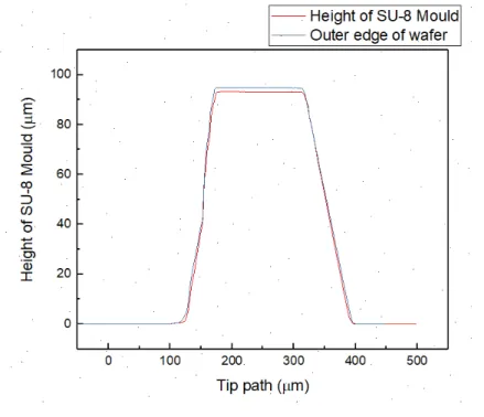
As seen in the profilometer (presented by the graph in Figure 11) the mould didn’t reach the 100 µm in height as expected, instead the top of the mould peaked around 93 µm in the middle of the Si wafer and 94 µm at the outer edges of the wafer. This gives an acceptable uniformity to the mould. The top of the ridge was approximately 100 µm wide for both ridges as in the mask. The slopes of the graph are caused by the width of the measuring tip.

(38)

The final devices were successfully sealed to the glass if after the exposure to Oxygen plasma the PDMS cannot be removed from the glass. And if there is no sign of distortion on the channels, this distortion can originate from the few seconds of pressure by hand that are applied to the PDMS after the exposure. In Figure 12 bellow it’s presented a successfully produced device.

Figure 12 Complete droplet generator, Y-Junction in this case. An individual photo of all droplet generator chips can be found in Appendix D.

3.3 COMSOL Simulation Results

To first understand the behaviour of the junctions COMSOL Multiphysics simulation software was used. The first junction that was simulated was the X100 that would serve as the standard to all other tests. For the X-Junction, a geometry was designed in the shape of a cross having the water being fed from the top and the oil to be fed from the sides as seen in Figure 11. For the T-Junction the water is fed from the side channel and the oil is fed from the top, as seen in Figure 12. In both geometries the walls were defined as PDMS, using the material library available in the software itself.

Although COMSOL does not require the Reynolds number to be introduced directly it is necessary to obtain this value to feed the software other variables such as Entrance Length (Le). Entrance length is the development distance that the flow takes to become fully developed in a pipe, that is the area following the pipe entrance where the interior wall of said pipe affects the flow of the expanding surface between the fluids and the wall [21]. These values must be calculated for the silicone oil and for water independently, as well as for each flow rate.

𝑅𝑒(𝑂𝑖𝑙) =𝜌 × 𝑢 × 𝐿_𝜇 =960 × 4 × 10_{48 × 10}−3× 100 × 10₋₃ −6= 8 × 10−3

For a silicone oil flow rate of 0.25 µL/min, present in the side channels, we obtain a value smaller than 1, well within the range that characterizes microfluidic systems. This value was chosen for being the smallest flow rate in a single channel, and because all other values used were multiples of 0.25.

The calculated Le was then given by [21],

𝐿𝑒 ≈ 0.06 × 𝑅𝑒 × 𝐿 = 4.8 × 10−8_𝑚

This value was then inputted into the software.

The calculated parameters required by the software to be able to correctly function were the Le of both

water and the silicone oil of 50 cSt.

(1)

(39)

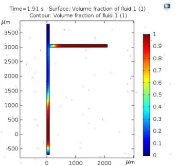
The objective of this simulation was to ascertain if the proposed channel dimensions and flow rates were capable of forming droplets, and as seen by Figure 13 and 14 that was achieved. Having the simulation presented the formation of droplets after the junction point.

Figure 13 Frame of simulated X-Junction 100 µm wide, at 2.0 µL/min. The water is presented in red and the oil in blue, the interface is presented in yellow because the chosen mesh is a coarser grid in order to speed up simulations. This means that the interface is presented as a mixture of water and oil, instead of a clear and abrupt phase difference.

For the simulated T-junction (T100) the result is as for the X100 junction a series of GIFs for each flow rate. The resulting GIFs present droplets forming, however the droplets were being formed downstream of the junction point without connexion to the channel forcing water into the junction.

(40)

3.4 Droplet Dimensions

As mentioned before for volume calculations a droplet is considered divided in three parts, the front and the back forming two half spheres with a diameter the same as the width/weigh of the channel, this part is considered the same for all channels of the same size, and a middle part that can take a form somewhere between a perfect cylinder and a perfect rectangular block.

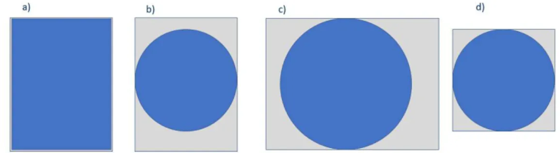
Since there was no way to visualize and confirm the shape that the droplet takes in the channels, two volumes were calculated, one assumed to be the maximum and the minimum volumes possible a droplet could take. For the maximum volume it is considered that the droplet is composed by a sphere, half in each end of the droplet, and a parallelepiped that fills all corners of the channel this corresponds to the first picture in Figure 15. For the minimum possible volume, it is considered the volume of a pill, that is two half spheres and a cylinder barely touching the wall of the channel, this corresponds to the three last pictures in Figure 15. The sphere has the same diameter as the cylinder in both the maximum proposed volume and the minimum.

Figure 15 Assumed front views of the droplets a) Maximum channel occupation possible corresponding to maximum possible volume on any channel; b) Minimum occupation of the main channel for the 50µm wide channel; c) Minimum occupation of the main channel for the 150µm wide channel; d) Minimum occupation of the main channel for the 100µm wide channel;

The graphs bellow present the estimated volumes for each geometry of droplet generator at different dispersed phase flow rates. It is important to note that the due to limitations of the infuser set up the continuous phase of the X-Junctions presented only one inlet, therefore the same flow rate for both inlets of each device. But for the continuous phase the flow is separated into the two side channels meaning that the flow rate of each independent side channel is half of what was introduced into the inlet.

In almost all configurations a target of droplets inferior to 10 nL was achieved, having the smaller estimates of volume reached bellow the nanolitre mark for the smallest geometry produced (50 µm), this means that as expected for the same type of junction, the size of the channels affects the size of the droplets.

3.4.1 X100 Junction

(41)

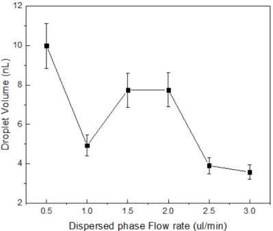
expected pattern of this type of junction, which was expected to deliver increasingly smaller droplets with the increase of the flow rate. As seen in Figure 16, bellow, there is a distortion effect clearly noted starting at those two points, making these obtained values quite unreliable. A possible explanation for this behaviour could be the effect of the drag of the wall. To try and avoid this effect the use of surfactants in the water can be a probable option.

Figure 16 Range of droplet volumes for droplet for the X-Junction 100 µm wide, in these graphs the error bars represent the maximum and minimum possible volumes that were calculated, and the point represents the average volume of those calculations.

(42)

Figure 17 Frames of the captured film of the 100 µm wide X- junction at different flow rates, from left to right, top to bottom 0.5 µl/min to 3.0 µl/min. The first given scale applies to the first two panels (0.5 ul/min and 1.0 ul/min) and the second applies to the remaining panels.

3.4.2 X50 Junction

This junction was tested to access the effect of channel size on the droplet volume. The 50 µm junction is the smallest of all the designs, making it more likely to achieve the smallest volumes. In this junction, the increase of the flow rate, had a clear effect on decreasing the droplet volume as can be seen in the graph in Figure 18. This is the only design that reaches a droplet volume bellow the nanolitre mark, given the minimum possible volume, at the two fastest flow rates (2.5 µL/min and 3 µL/min).

(43)

This junction suffered from the same problem as the X100, as seen in Figure 19, with the droplets inside the channel forming a long and thin thread before the first turn, probably due to irregularities inside the channel before the first turn. As in the X100 the use of surfactants can be a way to eliminate this effect. The droplets had to be measured right after the junction, because that was the only location where they were visible. In this droplet generator, the size of the droplets behave as expected, becoming increasingly smaller with an increasingly faster flow rate. This junction produced droplets in the dripping regime for all the flow rates that were tested.

Figure 19 Frames of the captured film of the 50 µm wide X- junction at different flow rates, from left to right, top to bottom 0.5 µl/min to 3.0 µl/min

3.4.3 Y100 Junction

(44)

Figure 20 Range of droplet volumes for droplet for the Y-Junction 100 µm wide

In the Y-Junction is important to note that this type of junction does not suffer from the same design limitation presented by the X-Junctions, because there is no need to make an inlet feed two channels, although there is still the limitation of inlet independence. This means that both inlets are always at the same flow rate.

When visualized on video where the frames from Figure 21 were obtained the droplet formation occurs far past the point of junction, this is a clear indicator of the junction working in a jetting regime.

(45)

3.4.4 X100-cont50 Junction

To compare the effects of different sized side channels a junction with smaller side channels was produced and tested. Although the side channel width is half of the previous, the flow rate is maintained because the syringe keeps injecting the same constant amount per minute independent from the channel. The change in behaviour is that the flow now passes through a smaller portion of the junction, increasing the shear stress on the dispersed phase.

When comparing these results with the standard X100 junction in Figure 22 we observe a more constant behaviour and a smaller droplet size, which is an advantage of reducing the channels width at the junction.

Figure 22 Range of droplet volumes for droplet for the X-Junction 100 µm wide with side channels 50 µm wide.

Aside from the volume reduction of the droplets another consequence of the reduction of the channels width was the increase of the generation rate, although not possible to determine, the fact that the USB microscope recorded droplets moving in the reverse direction when the flow rate was 1.5 µL/min means that the generation rate of droplets is superior to 30 droplets per second, given that the capture rate of the USB microscope is 30 fps. Although the 2.0 µL/min flow rate presents a drastic dip in volume all other volumes present values near each other, meaning that the main consequence of this design is an increase of generation rage. Along with a more uniform droplet generation it was also observed a more consistent spacing between droplets (plugs). This means that the especially for faster flow rates the agglomeration seen in the previous X-Junctions was avoided.

(46)

Figure 23 Frames of the captured film of the 100 µm wide X- junction with 50 µm wide side channels at different flow rates, from left to right, top to bottom 0.5 µl/min to 3.0 µl/min.

3.4.5 X100-fun50 Junction

The functionality of a flow focusing device was tested with the junction X100.fun50, this junction has a 50 µm wide entry to the main channel after the junction, this entry is 150 µm long and has a 150 µm long widening to the 100 µm of the main channel. When compared to the X100.cont.50 junction we observe in the graph in Figure 24, larger droplets for the slower flow rates but smaller when a faster flow rate is used. This junction presents a clear decrease in volume with the increase of the flow rate, as expected of a X-Junction.

(47)

The generation behaviour was of the squeezing type for the smaller of the flow rates (0.5 µl/min to 1.5 µL/min) and appear to change to dripping type for the rest of the flow rates, however the obtained droplet size does not match this regime. Since if this was a clear dripping regime the droplets should have a smaller size than the width of the funnel, but as seen in Figure 24 the droplets are larger in every dimension than the width of the funnel. On the other hand, since the length of the funnel was larger than most used flow-focusing devices there may be an effect on the droplet size passing through the funnel.

When watching the recording of the X100-fun.50 it is clear that at starting at the 1.5 µL/min flow rate the recordings suffer the stroboscopic effect, having the droplets move opposite to the flow’s direction. This means a generation rate superior to 30 droplets per second since the USB microscope has a capture rate of 30 fps. It can also be seen in Figure 25 a greater uniformity of plugs and droplets between droplets at faster flow rates.

Figure 25 Frames of the captured film of the 100 µm wide X- junction with 50 µm wide flow-focusing device at different flow rates, from left to right, top to bottom 0.5 µl/min to 3.0 µl/min.

3.4.6 X100-60º Junction

(48)

value above the targeted range (10 nL to 1 nL). This might mean that the entry angle of the side channel’s flow rate doesn’t affect slower flow rates, but this can only be confirmed by testing slower flow rates that 0.5 µL/min.

Figure 26 Range of droplet volumes for droplet for the X-Junction 100 µm wide with side channels joining the main channel at a 60º angle

This junction presents a less erratic behaviour than the X100 junction. However, as can be seen in Figure 27 (especially for the 1.5 µL/min flow rate), a small distortion exists in the droplets after the first turn but disappears after the second turn. These distortions affect the beginning and end of the droplet, as they are not rounded but present a elongation towards the previous and next droplet. This can be due to imperfections of the turns that may be slowing the flow more on one side of the channel than on the other. But are counteracted on the second turn, evening the droplet.

(49)

Figure 27 Frames of the captured film of the 100 µm wide X- junction with side channels joining at a 60º angle to the dispersed phase channel at different flow rates, from left to right, top to bottom 0.5 µl/min to 3.0 µl/min.

3.4.7 X150 Junction

The largest produced geometry is the one that should have produced the largest droplets, as can be seen in Figure 28, if it wasn’t for the unexpectedly large droplets produced by the X100 and the X100.60 junctions. But since those junctions present a distortion of the droplets the values might not be viable to compare to the X150 junction. This junction at the lowest flow rate reached a droplet volume above the established goal of the 10 nl limit. But despite that the slower flow rates the droplet size have probable volumes in the same range, not suffering the expected reduction in size with the increase of the flow rate.

(50)

This junction presents two working regimes, jetting for the smallest flow rates, 0.5 µl/min and 1 µl/min, having the droplets break almost 1.5 mm after the junction point for the last one and more than 2 mm after the junction for the 0.5 µm/min, as seen in Figure 29. For the other flow rates the droplets were produced in the dripping regime. However, for the 2.5 µL/min and 3 µL/min the capture rate of the USB microscope could not record the correct movement of the droplets, recording them moving backwards and upstream towards the inlets, this is another example of the stroboscopic effect.

Figure 29 Frames of the captured film of the 150 µm wide X- junction at different flow rates, from left to right, top to bottom 0.5 µl/min to 3.0 µl/min.

3.4.8 T100 Junction

(51)

Figure 30 Range of droplet volumes for droplet for the T-Junction 100 µm wide

When analysing the recorded clips and frames from Figure 31 of the working junction, two regimes can be distinguished, the squeezing regime for the smaller flow rates (0.5 µl/min and 1 µl/min) and dripping regime for the remaining flow rates. The squeezing regime originated droplets that are noticeably larger than the ones originated by dripping. As said previously this design’s simplicity leads to well defined regimes and doesn’t give origin to droplet distortions as in some X-junctions.

Figure 31 Frames of the captured film of the 100 µm wide T- junction at different flow rates, from left to right, top to bottom 0.5 ul/min to 3.0 ul/min

(52)

[13] [15] do not recognize a squeezing regime for this type of junction. However, in terms of appearance some of the dripping regime resemble a squeezing regime more closely. All volume graphs can be seen in Figure 32.

Table 3 Combined observed regimes for each junction; D – Dripping; D* – Classified as Dripping but resembles other regime more closely, namely squeezing; S – Squeezing; J – Jetting.

Flow Rate (µL/min)

0.5 1 1.5 2 2.5 3 Minimum

volume Po

X100 D* D* D* D* D* D*

X50 D* D* D* D* D D

Y100 J J J J J J

X100-cont50 D* D* D D D D

X100.fun50 S S S D D D

X100.60º D* D* D* D* D* D*

X150 J J D* D* D* D*

T100 S S D D D D

(53)

4. Conclusions and Future Perspectives

The foreseen objective of this thesis, the production of droplet generators capable of producing W/O droplets smaller than 10 nL, was achieved in all generators, with the exception of the slower flow rates of the X100, X150 junctions and X100.60º. When comparing all the generators we observe that the smaller droplets were observed in the smallest design, but among the same type designs we observe an advantage when producing smaller droplets if other components are added to the junction. Flow-focusing devices present a good addition for faster flow rates.

For X type junctions, faster flow rates represent smaller droplets. This is as expected for this type of junctions [2]. The times that this was not true were for the devices that presented some sort of problem (X100) or some design alteration (X100-cont50). The X150 junction despite presenting a larger volume for the 3.0 µL/min flow rate than the 2.5 µL/min when comparing all the volume droplets, shows a slight tendency for a decrease in volume can be noted, the same applies for the X100.60º junction.

The smaller droplets obtained are formed under the dripping regime, however some of these dripping regimes when visualized do not resemble the description of a dripping regime. This dripping regimes are marked in Table 3 as “D*”. Instead of the dispersed phase break into a droplet as soon as it enters the junction, this phase continues to fill past the main channel junction until the pressure of the two opposing flows from the side channels causes the breaking of the dispersed phase into a droplet. After the break-up a retraction of the side channels flow is also observed. The final droplet is limited by the size of the channel, not being round. This falls in line with what is described in more recent papers [22], however the jetting regime is used interchangeably with the dripping regime. These regimes resemble more closely a squeezing regime, having the continuous phase squeeze the dispersed phase at the junction point. Other description of droplet formation in squeeze regime in X-Junctions is given by P. Zhu and L. Wang in their review, describing it as a result of build-up of the pressure gradient caused by the continuous phase coming from the side channels, increasing the gap between the forming droplet and the rest of the dispersed phase flowing from the inlet [8].

The COMSOL simulations were successful when first obtained, having been achieved droplets for the X100 junction, and allowed to determine the dimensions of the channels within the chips and flow testing conditions to be used in the experimental tests of the produced devices. It is clearly an extremely useful tool for microfluidic design and testing, and in future it is a valid way to optimise the droplet generation process to avoid the mass production of useless devices.

(54)

addition of surfactants to the aqueous phase can also be a way to avoid the dephasing of the droplets after their formation. A better designed turn and S curves, so that there is little distortion of the velocity after entering the turn.

(55)

References

[1] T. M. Squires and S. R. Quake, “Microfluidics: Fluid physics at the nanoliter scale,” Rev. Mod. Phys., vol. 77, no. 3, pp. 977–1026, 2005.

[2] S. Teh, R. Lin, L. Hung, and A. P. Lee, “Droplet microfluidics,” Lab Chip, vol. 8, no. 2, p. 198, 2008.

[3] S. Thomas, R. L. Orozco, and T. Ameel, “Microscale thermal gradient continuous-flow PCR: A guide to operation,”

Sensors Actuators, B Chem., vol. 247, pp. 889–895, 2017.

[4] G. Perkins, H. Lu, F. Garlan, and V. Taly, “Droplet-Based Digital PCR,” vol. 79, pp. 43–91, 2017.

[5] M. U. Kopp, A. J. De Mello, and A. Manz, “Chemical Amplification : Continuous flow PCR on a chip,” Science (80-. )(80-., vol(80-. 280, no(80-. May, pp(80-. 1046–1048, 1998.

[6] H. W. A Manz, N Graber, “Miniaturized Total Chemical Analysis Systems: a Novel Concept for Chemical Sensing,”

Sensors actuators B Chem. 1990, vol. 17, no. 6, pp. 620–624, 1995.

[7] J. Wu, W. Wen, and P. Sheng, “Smart electroresponsive droplets in microfluidics,” Soft Matter, vol. 8, no. 46, pp. 11589–11599, 2012.

[8] P. Zhu and L. Wang, “Passiveand active droplet generation with microfluidics: a review,” Lab Chip, vol. 17, no. 1, pp. 34–75, 2017.

[9] P. Garstecki, a M. Gañán-Calvo, and G. M. Whitesides, “Formation of bubbles and droplets in microfluidic systems,”

Bull. Polish Acad. Sci., vol. 53, no. 4, pp. 361–372, 2005.

[10] P. Garstecki, M. J. Fuerstman, H. A. Stone, and G. M. Whitesides, “Formation of droplets and bubbles in a microfluidic

T-junction—scaling and mechanism of break-up,” Lab Chip, vol. 6, no. 3, p. 437, 2006.

[11] Jw. and H. A. S. J K Nunes, SSH Tsai, “Dripping and jetting in microfluidic multiphase flows applied to particle and fibre synthesis,” J. Phys. D. Appl. Phys., vol. 114002, 2013.

[12] L. A. Gordon, Chistopher; Shelley, “Microfluidic methods for generating continuous droplet streams,” J. Phys. D. Appl. Phys., vol. 319, 2007.

[13] G. T. Vladisavljević, I. Kobayashi, and M. Nakajima, “Production of uniform droplets using membrane, microchannel and microfluidic emulsification devices,” Microfluid. Nanofluidics, vol. 13, no. 1, pp. 151–178, 2012.

[14] T. Fu, Y. Wu, Y. Ma, and H. Z. Li, “Droplet formation and breakup dynamics in microfluidic flow-focusing devices:

From dripping to jetting,” Chem. Eng. Sci., vol. 84, pp. 207–217, 2012.

[15] J. Tan, J. H. Xu, S. W. Li, and G. S. Luo, “Drop dispenser in a cross-junction microfluidic device : Scaling and mechanism of break-up,” Chem. Eng. J., vol. 136, pp. 306–311, 2008.

[16] M. De menech, P. Garstecki, F. Jousse, and H. A. Stone, “Transition from squeezing to dripping in a microfluidic

(56)

[17] S. L. Anna and H. C. Mayer, “Microscale tipstreaming in a microfluidic flow focusing device,” Phys. Fluids, vol. 18, no. 12, 2006.

[18] COMSOL INC., “COMSOL Multiphysics,” 2018. [Online]. Available: https://www.comsol.com/products. [Accessed: 01-Oct-2018].

[19] COMSOL INC., “COMSOL Multiphysics,” 2018. [Online]. Available: https://www.comsol.com/multiphysics.

[Accessed: 25-Oct-2018].

[20] J. B. Boreyko, G. Polizos, P. G. Datskos, S. A. Sarles, and C. P. Collier, “Air-stable droplet interface bilayers on

oil-infused surfaces,” Proc. Natl. Acad. Sci., vol. 111, no. 21, pp. 7588–7593, 2014.

[21] F. P. Incropera, D. P. DeWitt, T. L. Bergman, and A. S. Lavine, Fundamentals of Heat and Mass Transfer. 2007.

[22] S. Van Loo, S. Stoukatch, M. Kraft, and T. Gilet, “Droplet formation by squeezing in a microfluidic cross ‑ junction,”

(57)

Appendix A

Table 4 Estimated volumes for the 100µm wide X-Junction

X100

Dispersed phase Flow rate (µL/min) 0.5 1 1.5 2 2.5 3

Minimum Volume (nL) 8.851 4.398 6.874 6.882 3.499 3.208

Maximum Volume (nL) 11.126 5.456 8.609 8.620 4.312 3.942

X 50 Dispersed phase Flow rate

(µL/min)

0.5 1 1.5 2 2.5 3

Minimum Volume (nL) 2.24

9

1.887 1.402 1.235 0.896 0.882

Maximum Volume (nL) 2.84

6

2.385 1.767 1.555 1.123 1.106

Table 6 Estimated volumes for 100µm wide Y-Junction

Y100

Flow rate (µL/min) 0.5 1 1.5 2 2.5 3

Table 7 Estimated volumes for X-Junction with 100 µm of width in the main channel and 50 µm of width in side channels

X100 cont. 50

Minimum Volume (nL) 1.73

5

1.693 1.640 1.459 1.745 1.673

Maximum Volume (nL) 2.01

8

1.965 1.891 1.674 2.033 1.944

Table 8 Estimated volumes for the 100µm wide X-Junction with a flow-focusing funnel 50µm wide after the junction point

x100 fun 50

Table 9 Estimated volumes for the 100µm wide X-Junction with side channels at a 60º angle with the main channel

X100-60º

X150

(58)

Table 11 Estimated volumes for the 100µm wide T-Junction

T100

Flow rate (µL/min) 0.5 1 1.5 2 2.5 3

Appendix B

(59)

Appendix C

Table 12 Used nomenclature for each designs and respective design

X100 or X-Junction 100 µm

X50 or X-Junction 50 µm

(60)

X100.cont50 or X-Junction 100 µm continuous phase (side channels) 50 µm

X100.fun50 or X-Junction 100 µm Funnel 50 µm

(61)

T100 or T-Junction 100 µm

Y100 or Y-Junction 100 µm

Appendix D

(62)

Figure 35 X50 junction PDMS chip

Figure 36 Y100 junction PDMS chip

(63)

Figure 38 X100.fun50 junction PDMS chip

(64)

Figure 40 X150 junction PDMS chip

(65)

Orientador: Professor Doutor Hugo Manuel Brito Águas, Professor Associado, FCT-UNL Co-orientador: Professor Doutor Rui Igreja, Professor Auxiliar, FCT-UNL

Francisco Bernardo Gomes Filipe de Matos

Development of microfluidic droplet generator

Orientador: Professor Doutor Hugo Manuel Brito Águas,

Professor Associado, FCT-UNL

Co-orientador: Professor Doutor Rui Igreja,

Professor Auxiliar, FCT-UNL

Acknowledgement

Abstract

Resumo

Abbreviations and Acronyms

Symbols

Table of Contents

List of Figures

List of Tables

Motivation and Objectives

1.

Introduction

1.1

Digital Polymerised Chain Reaction

1.2

Microfluidics

1.2.1

Droplet Formation

1.2.2

Junctions types

1.3

COMSOL

2.

Materials and Methods

2.1

Production Techniques

2.2

Characterisation Techniques

2.3

COMSOL Simulations

3.

Results and Discussion

3.1

Sample identification nomenclature

3.2

SU-8 Mould Development and Fabricated Devices

3.3

COMSOL Simulation Results

3.4

Droplet Dimensions

3.4.1

X100 Junction

3.4.2

X50 Junction

3.4.3

Y100 Junction

3.4.4

X100-cont50 Junction

3.4.5

X100-fun50 Junction

3.4.6

X100-60º Junction

3.4.7

X150 Junction

3.4.8

T100 Junction

4.

Conclusions and Future Perspectives

References

Appendix A

Appendix B

Appendix C

Appendix D

Appendix E