The Performance of Deterministic and
Stochastic Interest Rate Risk Measures:
Another Question of Dimensions?
∗
Lu´ıs Oliveira
BRU-UNIDE and ISCTE-IUL Business School
E-mail: [email protected]
Jo˜
ao Pedro Vidal Nunes
†BRU-UNIDE and ISCTE-IUL Business School
E-mail: [email protected]
Lu´ıs Malcato
Associa¸c˜
ao Portuguesa de Seguros
E-mail: [email protected]
∗Financial support by FCT’s grant number PTDC/EGE-ECO/099255/2008 is gratefully acknowledged.
†Corresponding author. Complexo INDEG/ISCTE, Av. Prof. An´ıbal Bettencourt, 1600-189 Lisboa,
The Performance of Deterministic and
Stochastic Interest Rate Risk Measures:
Another Question of Dimensions?
Abstract
The efficiency of traditional and stochastic interest rate risk measures is compared under one-, two-, and three-factor Gauss-Markov HJM term structure models, and for different immunization periods. The empirical analysis, run on the German Treasury bond market from January 2000 to December 2010, suggests that: i) Stochastic interest rate risk measures provide better portfolio immunization than the Fisher-Weil duration; and ii) The superiority of the stochastic risk measures is more evident for multi-factor models and for longer invest-ment horizons. These findings are supported by a first-order stochastic dominance analysis, and are robust against yield curve estimation errors.
Key words: Interest rate risk, asset-liability management, immunization strategies,
stochas-tic duration, HJM models, stochasstochas-tic dominance.
1
Introduction
Interest rate risk is a long-standing concern for financial institutions and academics, and several interest rate risk measures have been derived to quantify this particular risk expo-sure. The development of interest rate risk measures dates back to Macaulay (1938), who introduces the concept of duration as a summary measure for the life of a bond. Hicks (1939) proposes the same measure but in the form of an elasticity of capital value with respect to the discount factor, and calls it the average period. Samuelson (1945) derives an average
time period, which corresponds to the Macaulay’s duration. Redington (1952) proposes the
classic immunization rules for protecting the surplus of a fixed income portfolio from changes in interest rate levels.
Fisher and Weil (1971) relax the Macaulay’s assumption of a flat yield curve, and develop a new duration measure—the Fisher-Weil duration—in which the discount factors are derived from the current term structure of interest rates. According to Fisher and Weil (1971), a portfolio is immunized against interest rate changes if the holding period return of the portfolio is at least as large as the holding period return of the target bond.1 However, it
is well known that the Fisher-Weil duration provides an accurate hedging only for parallel shifts of the yield curve.
To address the Fisher and Weil (1971) limitation of additive shifts in the yield curve, Bier-wag and Kaufman (1977) define a different duration measure. They assume an immunization approach in which changes in the term structure of interest rates occur in a multiplicative fashion, rather than additively. The resulting measure of duration was compared with those of Macaulay and Fisher-Weil for bonds of various coupons and maturities, but negligible differences were found for maturities lower than 20 years.
The severity of the assumptions underlying the previous duration models motivated the development of measures of dispersion, which emphasize the role that the portfolio structure possesses on the results of an immunization strategy. These measures of dispersion include
1The target bond is the zero-coupon bond, free of default risk and noncallable, that matches the investor’s
both the M -squared suggested by Fong and Vasicek (1984), and the M -absolute proposed by Nawalkha and Chambers (1996).2
Fooladi and Roberts (1992) as well as Bierwag et al. (1993) study the Canadian gov-ernment bond market, and analyze also the importance of portfolio design for the success of duration-based immunization strategies. They conclude that forcing a duration-matching portfolio to include a bond with a maturity that matches the length of the immunization period minimizes the deviation from the portfolio’s promised return. Similarly, Soto (2001) studies the Spanish government debt market in the period 1992-1999, and also concludes that the portfolio structure is non-trivial for immunization purposes; she finds that when portfolios include a bond maturing near the end of the holding period, the exposition to non parallel shifts of the term structure of interest rates drops notably. More importantly, and using again the Spanish government bond market, Soto (2004) tests the performance of a wide set of strategies,3 and concludes that the success of duration-matching strategies is primarily attributable to the number of factors considered. Similar findings are also reached by Bravo and Silva (2006) using data for the Portuguese government debt market, over the sample period from August 1993 to September 1999.
In opposition with the previous deterministic interest rate risk measures, the so called stochastic approach assumes that uncertainty about future interest rates is not fully captured by the current yield curve. This dynamic approach—initiated by the single-factor setups of Vasiˇcek (1977) and Cox et al. (1985)—includes both equilibrium and no-arbitrage mod-els. Equilibrium models require assumptions about key economic variables and the market prices of risk involved in the stochastic processes driving interest rates. No-arbitrage models overcome this difficulty by featuring an appealing built-in consistency with respect to the observed yield curve. Heath et al. (1992) (HJM henceforth) establish a general arbitrage-free
2Other popular approaches include the parametric duration models of Cooper (1977), Bierwag et al.
(1987), Chambers et al. (1988), or Prisman and Shores (2004), the partial duration models of Reitano (1990), and the key-rate duration model of Ho (1992).
3The strategies analyzed by Soto (2004) include a naive strategy, a maturity strategy, a minimum M
-absolute strategy, bullet and barbell portfolios, and four sets of strategies based on four multiple factor duration models.
framework, based on the evolution of instantaneous forward rates over time, and show that the initial yield curve and the interest rate volatility function are the only necessary inputs for pricing purposes.
As discussed by Ingersoll Jr. et al. (1978) or Cox et al. (1979), the traditional Macaulay and Fisher-Weil risk measures are not consistent with any reasonable arbitrage-free dynamic term structure model. Taking the short-term interest rate as the only state variable, Cox et al. (1979) introduce the concept of stochastic duration to measure the relative basis risk of bonds.4 Stochastic duration is defined as the time to maturity of a zero-coupon bond with
the same basis risk as the target coupon-bearing bond. This risk measure can accommodate multiple interest rate shocks, independently of the shape and/or location of the changes in the yield curve.
Gultekin and Rogalski (1984) use actual U.S. market data (between January 1947 and December 1976) to test empirically seven different duration specifications as measures of basis risk;5 they find that none of the duration measures tested is useful for fixed-income
performance evaluation and, hence, a duration-based immunization strategy may, in practice, not work. Moreover, Wu (2000) modifies the stochastic duration underlying the Vasiˇcek (1977) and Cox et al. (1985) models—by taking as the relevant risk factor the zero-coupon bond yield associated to a fixed fraction of the underlying coupon-bearing bond time to maturity—but is not able to consistently outperform Macaulay’s duration in the Belgian government debt market (between 1991 and 1992).
Au and Thurston (1995) derive duration measures under a one-factor HJM model, and define the basis risk of a coupon-bearing bond as a function of forward rate volatilities, as-suming constant, constant decay, and exponential decay volatility structures. Jeffrey (2000) also describes the relationship between duration measures and the forward rate volatility structure of HJM models. Munk (1999) generalizes the Cox et al. (1979) basis risk measure
4Basis risk can be defined as the relative change in the price of a bond due to an unexpected change in
the short-term interest rate.
5The seven specifications used by Gultekin and Rogalski (1984) were the durations of Fisher and Weil
(1971), Bierwag (1977), Khang (1979), three mesures of duration derived by Cooper (1977), and the single-factor stochastic duration proposed by Cox et al. (1979).
and derives general properties of the stochastic duration measure. Ho et al. (2001) compare the performance of a delta neutral hedge (based on a one-factor HJM exponential decay volatility model), a spot rate sensitivity-based hedge, and a modified duration hedge. Using weekly prices of three months sterling futures contracts—from December 1991 to December 1998—they hedge one-year sterling futures positions with two-year sterling futures contracts, and the results suggest that the delta-hedging strategy is not superior to a modified duration hedge. More recently, and using simulated data, Agca (2005) concludes that the traditional interest rate risk measures provide, in most cases, a similar or better immunization perfor-mance than the more complex (but single-factor) HJM interest rate risk measures.
Given the divergent results provided by the previous literature and summarized above, the main purpose of this study is to answer the following research questions: Are stochastic interest risk measures superior to their deterministic counterparts? Does the answer to the previous question depend on the dimension of the stochastic term structure model adopted? To test these two research hypothesis, we compare the immunization performance of the Fisher-Weil versus stochastic duration measures, by fitting the term structure of German Treasury interest rates through a parametrization that is consistent—along the lines of Bj¨ork and Christensen (1999)—with a Gaussian HJM model with one, two, and three factors. We also test a wide range of random, bullet and barbell portfolios, using investor planning periods of one, three, and five years. For this purpose, and although there are several immunization criteria that can be adopted, we focus on the most widely used approach: the duration matching criteria.
This paper proceeds as follows. Section 2 describes the method adopted to estimate the yield curve, the bond data set in use, and the quality of the estimated results. Section 3 details the theoretical issues behind the interest rate risk measures and the immunization strategies used in this paper. Section 4 discusses the main empirical implementation is-sues. Section 5 reports our results, and Section 6 tests their robustness. Finally, Section 7 concludes.
2
Term structure extraction methodology
All bonds to be considered are (almost surely) credit-risk free and provide a stream of certain cash flows at known times in the future. The ith observed time-0 bond price is denoted by
Bi(0). This bond provides future cash flows ci,j at times tj, for j = 1, ...mi. The fitted bond
price will be expressed as bBi(0), and is given by the following static no-arbitrage condition
that is appropriate to a world without taxes, embedded options, or other frictions:
b Bi(0) = mi ∑ j=1 ci,jP (0, tj) , (1)
where P (0, tj) is the time-0 price of a unit face value and risk-free zero-coupon bond with
maturity at time tj (≥ 0).
As noted by Bliss (1997), because real markets (from which we collect our bond data) are not frictionless, in practice we do not assume an exact pricing relationship such as equation (1), but rather the following inexact relation from which we estimate the discount function:
Bi(0) = bBi(0) + εi, (2)
where εi is a random error term.
Many different functional forms can be used to estimate discount factors P (0, tj) from
the observed market prices of treasury coupon-bearing bonds—see, for instance, Jeffrey et al. (2006) for a survey. In this study, we adopt the Bj¨ork and Christensen (1999) parametriza-tion, which is consistent with a Gaussian and multi-factor HJM term structure model.
2.1
Bj¨
ork and Christensen (1999) parametrization
Bj¨ork and Christensen (1999) argue that the choice of the functional form for the initially “observed” forward interest rate curve should be consistent with the formulation adopted for the term structure model under use (in terms of both the number of Brownian motions and the volatility specification considered).
Bj¨ork and Christensen (1999, page 327) point out two reasons for such consistency re-quirement. First, if a given interest rate model is supposed to be subject to daily calibrations, it is important that, on each day, the parametrized family of forward rate curves that is fit-ted to bond market data is general enough to be invariant under the dynamics of the term structure model. Second, if a specific family of forward rate curves is shown to have the ability to efficiently recover the cross-section of bond prices observed in the market, then it makes sense to incorporate such implied yield behavior into the dynamics of the interest rate model used.
Similarly to Nunes and Oliveira (2007), this paper proposes a parametrization of the yield curve that is consistent with a Gaussian and multi-factor HJM term structure model. Such a model can be formulated in terms of risk-free pure discount bond prices, which are assumed to evolve over time—under the risk-neutral martingale measure Q that takes as numeraire the “money-market account”— according to the following stochastic differential equation:
dP (t, T )
P (t, T ) = r (t) dt + σ (t, T )
′· dWQ(t) , (3)
where r (t) is the time-t instantaneous spot rate,· denotes the inner product in Rk, and WQ(t)
∈ Rk is a k-dimensional standard Brownian motion. The k-dimensional volatility function
σ (·, T ) : [0, T ] → Rk, where 0 denotes the current time, is assumed to satisfy the usual
mild measurability and integrability requirements—as stated, for instance, in Lamberton and Lapeyre (1996, Theorem 3.5.5)—as well as the “pull-to-par” condition σ (u, u) = 0 ∈ Rk,∀u ∈ [0, T ]. Moreover, for reasons of analytical tractability, such volatility function is
assumed to be deterministic.
Following, for instance, Musiela and Rutkowski (1998, Proposition 13.3.2), it is well known that if the short-term interest rate is Markovian and the volatility function σ (·, T ) : [0, T ] → Rk is time-homogeneous, then the volatility function must be restricted to the analytical specification
σ (t, T )′ := G′· a−1·[Ik− ea(T−t)
]
, (4)
where Ik ∈ Rk×k represents an identity matrix, while G∈ Rkand a∈ Rk×k contain the model
time-independent parameters. The Gauss-Markov and time-homogeneous HJM model to be estimated is defined by equations (3) and (4).
As shown in Nunes and Oliveira (2007, Proposition 4), under the assumption that matrix
a is diagonal, the minimal consistent family (manifold) of discount functions which is
invari-ant under the dynamics of the HJM model described by equations (3) and (4) is defined by a mapping Γ :R2k× R + → R, such that Γ (z, T − t) ≡ P (t, T ) = exp { k ∑ j=1 zj aj [ 1− eaj(T−t)]+ k ∑ j=1 zk+j 2aj [ 1− e2aj(T−t)] } , (5) where zj represents the jthelement of vector z ∈ R2k, and aj defines the jthprincipal diagonal
element of matrix a. Parameters a and z can be estimated by minimizing the absolute percentage differences between a cross-section of market treasury coupon-bearing bond prices and the corresponding discounted values obtained by decomposing each government bond into a portfolio of pure discount bonds, which are parameterized in equation (5).
Under this general specification, the HJM model dimension will be set at one, two, and three factors. Hence, three, six and nine parameters will be used, respectively, in the discount factor specification (5).
2.2
Bond data set description
The bond data set used to estimate the spot yield curve was collected from Bloomberg, and consists of German coupon-bearing Treasury bonds bid and ask close prices of actual transactions recorded each day (end of session) during the period between January 2000 and December 2010.
To mitigate problems associated with distorted prices arising from bonds not actively traded during the sample period, the robust outlier identification procedure proposed by Rousseeuw (1990) is used to exclude from the sample all illiquid issues. On each day, the bid-ask spreads of all traded bonds are standardized using the sample median (location estimator) and the median of all absolute deviations from the sample mean (scale estimator). Whenever the standardized score of a specific bond is higher than a pre-specified cutoff value (defined here as 2.5), that bond is automatically excluded from the cross-section under analysis.
Furthermore, to avoid problems associated with bonds that become less liquid as they approach maturity—and following, for instance, Sarig and Warga (1989), D´ıaz et al. (2006), or D´ıaz et al. (2009)—treasury bonds with a residual maturity of less than three months are excluded from the sample. Finally, and to preserve the homogeneity of the data, we only consider fully-taxable, non-callable issues.
These filters leave us a total data set of 170 bonds, with an average number of 40 bonds per cross-section, between a minimum of 27, and a maximum of 73. The average number of bonds with a residual maturity lower than 2 years is 13; between 2 and 5 years there are, on average, 13 issues; 8 issues between 5 and 10 years; and 4 issues between 10 and 15 years. The average number of bonds with a residual maturity beyond 15 years is only 2.6
2.3
Estimation of the term structure of interest rates
On each sample day, the term structure of interest rates is estimated by determining the values of the parameters z ∈ R2k and a∈ Rk×k that minimize a maturity weighted mean
ab-solute percentage pricing error (WMAPE) that reflects the average of the maturity weighted differences between fitted and market coupon-bearing bond prices. As noted by Bliss (1997), pricing errors for longer maturities tend to be larger. Because of the observed heteroskedas-tic behavior of the pricing errors, and acknowledging the inverse relationship between bond prices and interest rates, Bliss (1997) suggests weighting the pricing errors using the inverse
6Note that the liquidity filter is only used for estimation purposes. When running the immunization
of the corresponding bond’s duration to prevent the errors of long-term bonds from dominat-ing the results. In this study, and because different duration measures will be compared, each absolute percentage pricing error is weighted by the inverse of the bond’s residual maturity:
W M AP E (t) := Nt ∑ i=1 |ei(t)| ωi(t) Nt , (6) where ei(t) = b Bi(t)−Bi(t)
Bi(t) is the time-t percentage pricing error of the i
th bond, ω
i(t) =
1/ (tmi− t), and (tmi − t) denotes the time to maturity of the i
th bond at time t. B
i(t) and
b
Bi(t) represent the “mid-quote” and the fitted prices, respectively, of the ith bond, whereas
Nt is the dimension of the cross-section of treasury coupon-bearing bonds at time t.
To obtain the yield curves, the parameters contained in equation (5) are estimated through the minimization of the WMAPE statistic (6). Throughout the empirical anal-ysis, all optimization routines are based on the quasi-Newton method, with backtracking line searches, described in Dennis and Schnabel (1996, Section 6.3).
[Please insert Table 1 about here]
Our results show that the adopted parametrization fits the discount functions implicit in the German government bond market very well, resulting in reliable and smooth yield curves for the sample period under analysis. To validate this assertion, the summary statistics of all absolute pricing errors associated to each end-of-month yield curve estimation, between January 2000 and December 2010, are presented in Table 1. To better understand the German term structure behavior, we split the full sample period into two sub-samples: the “before crisis” period, and the “during crisis” period. The before crisis period begins in January 2000 and finishes in July 2007, while the during crisis period extends from August 2007 to December 2010.7
7The onset of the financial crisis is generally accepted to be late July 2007. On August 2007, the European
Central Bank provided the first large emergency loan to banks in response to increasing pressures in the Euro interbank market.
The first four columns of Table 1 present the end-of-month yield curve estimation errors for the full sample period, using one-, two-, and three-factor specifications. During the overall sample period, the average mean absolute percentage pricing error (MAPE) generated by the HJM consistent parametrizations is equal to only 12.5 basis points (b.p.), 9.3 b.p., and 6.1 b.p., respectively, for one-, two-, and three-factor specifications. The maximum sample MAPE (21.3 b.p.) is observed for the single-factor model during the crisis period, while the minimum sample MAPE (0.6 b.p.) is offered by the three-factor model before the crisis period. As expected, the two-factor model reports a better performance than the one-factor version, but also yields fitting errors that are clearly higher than those observed for the three-factor parametrization. The better performance of the three-three-factor specification is observed both in the pre-crisis (less volatile) and in the during crisis (more volatile) periods.
[Please insert Table 2 about here]
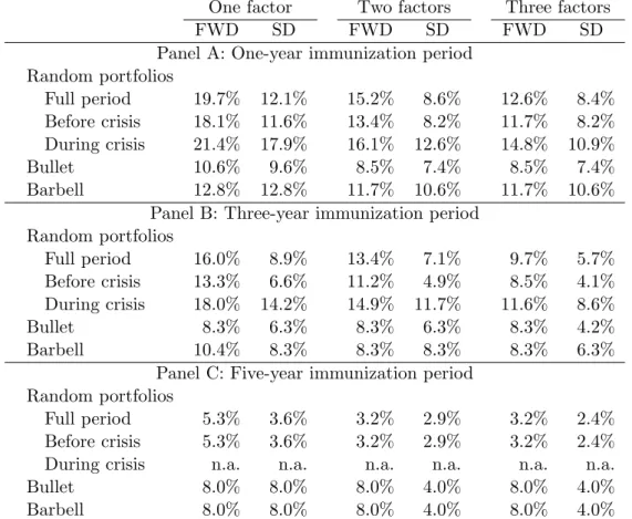
The summary statistics of the end-of-month one, three, and five years estimated spot interest rates are given in Table 2, and its levels are represented in Figure 1. During the overall sample period, the time-series of one, three, and five years spot rates display both high and low volatility regimes as well as diverse shapes. Hence, our data set should provide an interesting setting to test different immunization strategies.
[Please insert Figure 1 about here]
After the bursting of the dotcom bubble and the increased uncertainty following the terrorist attacks on September 2001, there was a phase of pronounced interest rate decreases until May 2003. Then, the German yield curve remained stable until September 2006. After December 2006, the first signs of increasing turmoil in global financial markets became visible, and a moderate reversal in the interest rates was observed until September 2008. During this period, the German interest rates increased substantially. Since December 2008, a generalized demand for safe assets, namely for German government bonds, took place. This global “flight to safety” trend depressed German bond yields more deeply than in any other Euro-zone country, and imposed a strong downward pressure on interest rates.
In summary, Figure 1 shows that not only the level but also the slope and curvature of the German yield curve have changed significantly during the sample period. This means that interest rates do not appear to be determined by a single risk factor, but rather by several factors that affect interest rates differently over the term structure.
2.4
Principal components analysis
In the previous subsection, the German spot yield surface was fitted through the parametric function (5) that is consistent with the interest rate dynamics generated by one-, two-, and three-factor HJM models. The goal of the present subsection is to provide empirical support that confirms the choice of three as the maximum number of non-trivial factors needed to reproduce almost all of the interest rates variance structure. For that purpose, a principal components analysis (PCA) is implemented.
The data consists of daily estimated continuously compounded spot interest rates for ten maturities, between one and 10 years, yielding a total of 3, 116× 10 data points, from January 04, 1999 to December 31, 2010. Since the implementation of the discount function parametrization (5) requires the previous specification of the number of model factors (k), the spot interest rates were reestimated—for PCA purposes only—through the Nelson and Siegel (1987) parametrization of the yield curve.
The PCA was performed not on the interest rate levels but rather on the daily interest rate changes, since the latter were checked to be stationary. Then the eigenvalues and the eigenvectors associated with the sample correlation matrix of the spot interest rates changes were computed, being the eigenvectors scaled to the unit length, that is the eigenvectors, or loadings, matrix was computed as an orthogonal matrix. Finally, each factor—or “principal component”–was obtained as a vector of linear combinations between the loadings and the original data of spot interest rates changes.
Based on the eigenvalues of the sample correlation matrix, it is possible to compute the contribution of each principal component to the explanation of the overall interest rate variability. The first factor is found to explain 79.74% of the total sample variance. The
second and third factors possess a much lower, but still significant, explanatory power: 16.27% and 3.94%, respectively. Consequently, the first three factors, taken together, span almost 100% of the interest rate variability. Therefore, the number of independent linear combinations needed to summarize the dynamics of the yield curve, in its entirety, can be reduced, without much loss of information, to only three orthogonal factors. This empirical finding not only justifies the irrelevance of implementing HJM model specifications with more than three factors, but also raises doubts on the use of single-factor term structure models for immunization purposes—as done, for instance, by Wu (2000) and Agca (2005).
3
Interest rate risk measures
Considerable research has been undertaken to help protect institutional investors against the fluctuations of interest rates and of bond prices. Money managers, arbitrageurs, and traders need to measure the bond’s price volatility in order to implement hedging and trading strategies. The most commonly used measure is duration: it reflects the sensitivity of bond prices to a change in interest rates.
3.1
Traditional measures
The traditional or deterministic risk measure that we consider in this study is one of the most explored in the literature and by practitioners: the Fisher-Weil duration. As mentioned in Section 1, the concept of duration first used by Macaulay (1938) assumes the existence of a flat term structure that can change only by parallel shifts. Fisher and Weil (1971) relaxed the assumption of a flat yield curve and developed a new duration measure in which the discount factors are derived from the current term structure of interest rates. However, Ingersoll Jr. et al. (1978) show that the Fisher-Weil duration can only be a valid risk measure for parallel (i.e. shape preserving) shifts in the entire yield curve.
3.2
Stochastic measures
As argued by Cox et al. (1979), if we are interested in a dynamic duration statistic that can measure risk for multiple shocks of different magnitudes affecting the term structure of interest rates, then we need a measure that is consistent with the dynamics of the spot interest rates and, therefore, one that is derived under a reasonable stochastic interest rate term structure model.
According to equation (3), in this paper we consider a general interest rate term structure model where the evolution of bond prices is affected by changes in k independent standard Brownian motions. Following Munk (1999, Equation 2) and using the time-homogeneous specification of equation (4), the (multi-factor) stochastic duration D(t) for a coupon-bearing bond can be obtained as the implicit solution of the following equation:
k ∑ l=1 G2 l a2l [ 1− ealD(t)]2 = k ∑ l=1 G2 l a2l [ m ∑ j=1 w (t, tj)− eal(tj−t) ]2 , (7) where w (t, tj) := cjP (t, tj) ∑m j=1cjP (t, tj)
are weights which add up to 1, Gl is the lth element of vector G∈ Rk, al corresponds to the
lth principal diagonal element of matrix a ∈ Rk×k, and c
j are the cash flows generated by
the coupon-bearing bond at times tj > t (for j = 1, ..., m).
Equation (7) will be used in this study to compute the stochastic HJM durations for the one-factor (k = 1), two-factor (k = 2), and three-factor (k = 3) volatility specifications adopted. For this purpose, it is necessary to estimate the parameters G∈ Rk and a∈ Rk×k. The diagonal matrix a∈ Rk×k is obtained by fitting equation (5) to market prices of German
Treasury coupon-bearing bonds between January 2000 and December 2010.8 Then, the
8Since one year of data is required to estimate the parameters G∈ Rkdefining the HJM volatility function
(4), additionally we also had to estimate the interest rates term structure between January and December 1999.
volatility parameters G∈ Rk are computed daily by minimizing the differences between the
historical standard deviation of the one-year forward rate and the model volatility computed through equation (4).
3.3
Immunization strategies
The goal of an immunization strategy is to ensure today (time 0) that, at the end of a pre-specified time horizon (time th), and regardless what happens to the yield curve, the market
value of a bond portfolio will be no less than the market value that would be obtained if interest rates had not change; that is, the realized rate of return on the bond portfolio will be no less than the current spot rate for time th.
By forming, at time 0, a portfolio with a value equal to the present value of a future liability that matures at time th, the goal is to manage the portfolio in order to hedge that
unique future liability against yield curve changes. For that purpose, it is well known that it is only necessary to satisfy the following duration matching immunization rule:
Dp = th, (8)
where Dp is the portfolio duration.
The theoretical justification for the immunization rule defined in equation (8) is related to the concepts of reinvestment risk and price risk. A shift in the yield curve produces two symmetrical effects on the future value of a portfolio: the reinvestment effect and the price effect. The reinvestment effect captures the impact on the compounded value of the cash flows generated and reinvested up to the investment horizon (th), while the price effect
corresponds to the immediate impact on the portfolio market price of an interest rate change. When condition (8) is satisfied, the above symmetric effects are of the same magnitude, and the net impact is null.
However, the efficiency of this immunization rule is limited by the fact that, in order to maintain the immunization condition (8), the portfolio must be continuously rebalanced and, in the presence of transaction costs, such continuous rebalancing should penalize the
portfolio’s realized rate of return. Additionally, and no matter the duration measure used in equation (8), we are always confronted with the “risk of stochastic process”: For instance, the use of the Fisher-Weil duration in the immunization rule (8) is only efficient if the yield curve is driven only by parallel shifts, as described in Ingersoll Jr. et al. (1978) and Cox et al. (1979).
The goal behind the use of a stochastic duration measure is the same as for the Macaulay or Fisher-Weil durations: the measurement of the relative change in the price of a bond (or a portfolio of bonds) arising from an unexpected change in interest rates. This means that the immunization condition (8) still holds if we replace the Fisher-Weil duration by a stochastic duration measure.
Finally, note that only duration-matched immunization strategies will be run in this study. Since we will be working in continuous time, the convexity of the bond’s portfolio will be of order O(dt2) and, hence, should have no value.
4
Implementation issues
This section presents the methodological issues associated to the implementation of the immunization strategies tested. We specify three immunization horizons (of one, three, and five years) and divide the whole sample period into overlapping subintervals. Each planning period starts at monthly intervals on the last trading day. The opportunity set consists of all outstanding German government bonds.
4.1
Starting and rebalancing dates
The sample comprises the period from January 2000 to December 2010. To increase the number of holding period observations, we restart a new strategy every month. This means that there are a total of 120 overlapping starting dates for the one-year, 96 for the three-year, and 72 for the five-year planning horizons. Globally, we have tested a total of 38,370
portfo-lios whose duration matches exactly the respective immunization periods—as prescribed by equation (8).
For the entire sample period, each portfolio is rebalanced monthly (at the end of each month) as well as—following D´ıaz et al. (2009)—on every coupon payment date, by rein-vesting the cash flows generated by the bonds included in the portfolio. These procedures constitute important innovations since in the previous literature the portfolios are only re-balanced quarterly or semi-annually, and are not adjusted extraordinarily irrespective of the pattern of bond payments—see, for instance, Fooladi and Roberts (1992), Soto (2001, 2004), and Agca (2005)—or, at most, merely add the interim coupons obtained at the next rebalancing date—as in Bravo and Silva (2006).
4.2
Prices, bond selection and portfolio formation strategies
Since all immunization strategies will be tested under the presence of transaction costs, we use bid prices to evaluate the portfolio and to sell bonds, but ask prices to buy bonds at each rebalancing date. On the starting date of each immunization period, the bonds used in this study are filtered to ensure that only bonds that had already been traded by that date (i.e. bonds that already had their first settlement date and had not reached their maturity) were considered. Since the component bonds of each portfolio will be maintained throughout the entire immunization period, we need to prevent a component bond from maturing before the end of the last rebalancing interval. Henceforth, only bonds that expire no less than one month before the target date are considered to be combined with all the other bonds. Whenever these bonds expire, we sell the entire portfolio and buy a synthetic zero-coupon bond with a time to maturity equal to the residual immunization horizon.9
We run random, bullet and barbell portfolios at each starting date, and each of these portfolios is duration matched with the target zero-coupon bond. Random portfolios cor-respond to active portfolio management strategies and are formed using all the possible
9D´ıaz et al. (2009) use one-week repos and rebalance the portfolio weekly until the end of the holding
two-bond constituents amongst the available German Treasury bonds at each starting date. Bullet and barbel portfolios express passive immunization strategies and correspond, respec-tively, to the shortest and highest duration differences between the two bonds involved in all strategies that have started in each month.
4.3
Efficiency measure
To measure the efficiency of the immunization strategies to be analyzed in Section 5, we compute the following excess return (ERth
0 ) measure for all the tested immunization
portfo-lios:
ERth
0 := RRR
th
0 − rc(0, th) , (9)
where rc(0, th) is the continuously compounded spot rate given, at each starting date, by
the interest rate term structure model under use for a maturity equal to the immunization period (th = 1, 3, and 5 years), and RRRt0h is the portfolio realized rate of return which is
computed at the end of the immunization period as
RRRth 0 := ln ( Bp(th) Bp(0) ) th , (10)
where Bp(0) and Bp(th) are the initial and the final values of the immunized portfolio,
respectively. Note that when the excess return ERth
0 is greater than or equal to zero, the
liability is fully covered.
As mentioned in Section 1, this study only considers duration based immunization strate-gies. Two different risk measures are used to match the durations of the portfolios: the Fisher-Weil duration and the stochastic duration (under one-, two- and three-factor HJM specifications).
5
Empirical results
Table 3 summarizes the descriptive statistics of the excess returns—as defined in equation (9)—generated by duration matched portfolios based on the Fisher-Weil and on stochastic risk measures. Both risk measures are implemented under the Gaussian HJM model (3), using one, two, and three factors. Panels A, B, and C show the excess returns statistics for one-, two- and five-year immunization periods, respectively. Overall, we tested a number of portfolios that ranges from a total of 29,350, for the one-year, 7,391, for the three-year, and 1,629 for the five-year immunization horizons.
[Please insert Table 3 about here]
For all immunization horizons considered, and under any number of model factors, the use of a stochastic duration measure provides a better performance than the Fisher-Weil risk measure. The average and median excess return is always higher for the strategies based on a stochastic duration measure, whereas its standard deviation is usually lower (except for the three-year planning horizon when tested under a single-factor HJM model). For instance, under a three-factor HJM model and for the five-year immunization period, the average excess return obtained through a stochastic duration measure is 3 b.p. higher than the one produced via the Fisher-Weil duration, and the standard deviation of the excess return is 0.2 b.p. lower than the one associated to the deterministic duration measure. Moreover, the mean-difference comparisons (based on a one tail t-test) between the Fisher-Weil and the stochastic duration measures are not statistically significant at a 10 percent level only for the one- and two-factor specifications (in one- and three-year immunization horizons for the single-factor model, and in one-year strategies for two-factor models).
Under a three-factor HJM model, the independence of the average excess returns gen-erated by deterministic and stochastic duration measures is always rejected at a 10 percent significance level for one-year strategies and at a 5 percent level for longer immunization hori-zons. This means that the differences in performance between deterministic and stochastic duration measures are better captured under a multi-factor term structure model.
There-fore, this finding also explains the inability of the single-factor HJM model adopted by Ho et al. (2001) or Agca (2005) to compare the immunization performance of deterministic and stochastic risk measures.
The use of a more general three-factor specification not only highlights the superiority of the stochastic duration measure with respect to its deterministic counterpart but also provides a better immunization performance than the alternative lower-dimensional specifi-cations. For instance, through a stochastic duration measure and for the three-year immu-nization period, the three-factor HJM specification yields the highest average excess return (of 22.2 b.p.) and the lowest standard deviation (of 17.5 b.p.). Note that the superior per-formance of the three-factor HJM formulation is in line with, for instance, the findings of Soto (2004) and Bravo and Silva (2006), who show that the number of risk factors considered in the design of immunization strategies is of particular relevance. Furthermore, during our sample period, the frequent changes of the German yield curve shape—in particular after the start of the crisis period, when a twist and a strong upward steepening were observed—also favored the higher flexibility provided by a multi-factor specification.
Table 3 shows that the superiority of stochastic duration measures is stronger the longer the immunization planning horizon: For the five-year immunization period, the null hy-pothesis of a zero mean-difference is rejected at a 10 percent significance level even for the single-factor HJM specification. Moreover, longer planning horizons tend also to improve immunization performance: The highest average excess return for the one-year horizon is equal to only 18.8 b.p., which compares with 22.2 b.p. and 27.7 b.p. for the three-, and five-year immunization periods; moreover, the longer five-year horizon presents the lowest standard deviations (for all duration measures and under all model dimensions). This ev-idence supports previous studies—as, for instance, Soto (2004), Agca (2005) or Bravo and Silva (2006)—and suggests that duration-matching strategies are likely to work better for longer investment horizons. A possible explanation for the good performance of the longer immunization strategies lies in the relatively less rebalancing needs to ensure the duration matching condition.
[Please insert Table 4 about here]
Since we are mainly concerned with the downside risk associated to an immunization strategy, Table 4 reports the percentage of duration matched portfolios whose excess return— as defined in equation (9)—is negative, meaning that the liability coverage is not achieved. The second to seventh columns of Table 4 report the negative performance of the Fisher-Weil and stochastic risk measures, under the one-, two-, and three-factor HJM parametrizations. Panels A, B, and C show the results for the one-, three-, and five-year immunization horizons, respectively. To control whether the volatility changes that have been experienced during the sample period could affect the performance of the immunization strategies, we split the full period into two sub-periods. The “before crisis” period ranges from January 2000 to July 2007, when the markets experienced a lower volatility regime, while the “during crisis” period, covering August 2007 to December 2010, was characterized by dramatic changes in both the level and shape of the term structure.
Table 4 shows that the stochastic risk measures adopted encompass a lower downside risk than the Fisher-Weil duration. For all model dimensions and immunization periods, the percentage of portfolios with negative excess returns is always higher for the deterministic Fisher-Weil duration. For instance, under a three-factor HJM model and for the three-year immunization horizon, the percentage of unsuccessful immunization strategies is reduced from 9.7% to 5.7% when moving from the deterministic to the stochastic duration measure. For all immunization periods considered, and consistently with the results already pre-sented in Table 3, the three-factor HJM specification yields the lowest percentage of negative excess returns: For example, with a three-year planning horizon and using a stochastic du-ration measure, the percentage of portfolios with negative excess returns drops from 8.9% to 5.7% as we move from a single-factor to a three-factor HJM model. These results pro-vide further epro-vidence on the advantage of comparing the performance of deterministic and stochastic risk measures under a multi-factor formulation.
As expected, the percentage of unsuccessful immunization strategies is higher during the “crisis period” for all planning horizons, model dimensions and duration measures.
Never-theless, we still observe the same patterns as for the overall sample period: The stochastic duration measure implemented under a three-factor HJM specification yields the lowest per-centage of portfolios with negative excess returns.
To test the influence of the portfolio formation technique on the immunization perfor-mance, the bottom lines of Panels A, B, and C from Tables 3 and 4 summarize, respectively, the average excess returns and the percentage of portfolios with negative excess returns that are generated by the bullet and barbell strategies. The bullet portfolios clearly outperform barbell portfolios: The bullet strategies always yield higher average excess returns and less unsuccessful portfolios for all model dimensions, risk measures, and immunization periods. This overall better performance of the bullet portfolios is in accordance with the existing literature—see, for example, Fooladi and Roberts (1992) or Agca (2005)—and arises be-cause bullet portfolios have more cash flows centered around the planning horizon, yielding, therefore, a lower exposure to interest rate risk than for barbell portfolios.
In summary, Tables 3 and 4 show that immunization strategies based on a stochastic duration measure (derived from a multi-factor term structure model) provide superior per-formance against interest rate risk. This is an important finding for insurance or pension funds, i.e. investors that typically face long-term planning horizons, and to whom the avail-ability of more effective interest rate risk management tools is crucial.
6
Robustness tests
Our previous results show that the number of immunized portfolios that beat the expected rate of return (given by the initial spot rate for the planning horizon)—that is the number of positive returns obtained from equation (9)—is maximized when using a stochastic duration measure instead of its deterministic counterpart. This happens for all immunization periods, sub-samples, portfolio formation strategies, and model dimensions tested.
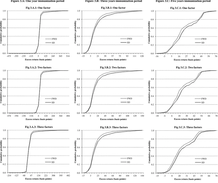
To evaluate the robustness of the previous empirical findings, we perform a stochastic dominance analysis to all the combinations tested, i.e. to the one-, two-, and three-factor HJM parametrizations implemented using both deterministic and stochastic duration mea-sures. Based on the cumulative distribution of the percentage returns (instead of average realized returns), this analysis provides additional evidence that immunization strategies based on stochastic duration measures lead to a superior performance. The results are plotted in Figure 2. Figure 2.A shows the cumulative probability frequencies for the one-year immunization period, using one-, two-, and three-factor HJM parametrizations of the yield curve. Figures 2.B and 2.C present the same frequencies for the three-, and five-year immunization periods, respectively.
Figure 2 shows that the probability of achieving a better immunization result is always greater with the stochastic rather than with the Fisher-Weil duration measure. For the three- and five-year immunization periods, the use of a stochastic HJM three-factor dura-tion guarantees first-order stochastic dominance over the use of the Fisher-Weil duradura-tion measure. For the one-year holding period, no clear first-order stochastic dominance is noted. Nevertheless, second-order stochastic dominance in favor of the stochastic duration approach is observed for this immunization period. Therefore, this results confirm that the superiority of the stochastic duration performance grows with the length of the immunization period considered.
[Please insert Table 5 about here]
In opposition with Agca (2005), we have tested different immunization rules using real market data instead of simulated bond prices. Therefore, the empirical evidence found against the use of deterministic duration measures cannot be attributed to its inconsistency with the interest rate HJM model dynamics adopted. However, it is then possible to argue that the yield curve estimation errors reported in Table 1 might be large enough to affect the performance of the risk measures tested.
In order to test if the outcomes of Tables 3 and 4 depend on the misfit of the spot yield curve, we estimate the following regression model for different investment horizons, different risk measures and different model dimensions:
M ean|ER (t)| = α + β × MAP E (t) + ε (t) , (11) where M ean|ER (t)| is the mean absolute excess return obtained from all immunization strategies starting at the end of month t, M AP E (t) is the corresponding end-of-month t mean absolute percentage pricing error associated to the yield curve estimation, and ε (t) is an error regression term. The results are reported in Table 5, and show that even at a 10 percent significance level, we cannot reject the null hypothesis H0: β = 0 for all immunization
periods, for all duration measures, and under any model dimension. Consequently, we may conclude that our results are robust against the noise associated to the estimation of the spot interest rates.10
7
Conclusions
The duration measures of Macaulay and Fisher-Weil are still widely used in practice, even though new risk measures have emerged through the rapid development of stochastic term structure models. Moreover, the empirical evidence on the performance and efficiency of these two groups of risk measures is mixed, with some empirical studies finding that tradi-tional deterministic duration measures perform at least as well as the stochastic risk measures derived from no-arbitrage term structure models.
The stochastic term structure model used in this study belongs to the popular arbitrage-free framework proposed by Heath et al. (1992). The hypothesis under study is that the risk measures implied by stochastic term structure models are more appropriate for immunization
10Following D´ıaz et al. (2008), we have also used the changes in the target rate of return (end-of-month
one-, three-, and five-year zero coupon yields) instead of MAPE as the explanatory variable, and the changes in the mean absolute excess returns as the explained variable, but the results are broadly similar to the ones presented in Table 5. To save space, those results are not reported here but are available upon request.
purposes than their traditional counterparts. For this purpose, this study compares the immunization performance of the Fisher-Weil duration with the stochastic risk measures derived from an yield curve parametrization that is consistent with a Gaussian and multi-factor HJM term structure model, as suggested by Bj¨ork and Christensen (1999). A duration matching strategy is considered, and we run a total of 38,370 portfolios among random, bullet and barbell strategies, during a sample period that ranges from January 2000 to December 2010.
The results obtained clearly suggest that stochastic risk measures outperform the tradi-tional Fisher-Weil duration for immunization purposes. Furthermore, we also conclude that the superiority of the stochastic duration measures is better captured under a multi-factor term structure model and for longer immunization periods. Note that these conclusions are based not only on the analysis of average excess returns and downside risks for each duration approach, but are also justified by a stochastic dominance analysis. We have also compared the influence of portfolio formation techniques on the average final return of the bond port-folio, and found that bullet portfolios tend to provide a better immunization performance than barbell strategies.
Our conclusions are in line with, for instance, Fooladi and Roberts (1992), Soto (2001) or Agca (2005) in respect to the prevalence of additional returns due to portfolio formation techniques, but diverge from Wu (2000) and Agca (2005) when comparing the performance of stochastic and deterministic duration measures. This divergence arises because Wu (2000) and Agca (2005) only use a single-factor term structure model while we test multi-factor HJM specifications.
Note that our analysis avoids any model bias that might favor HJM risk measures be-cause we compare all risk measures using real market data. Moreover, we also show that the superior performance of the stochastic duration measures is not driven by yield curve estimation errors.
References
Agca, S., 2005, The Performance of Alternative Interest Rate Risk Measures and Immuniza-tion Strategies under a Heath-Jarrow-Morton Framework, Journal of Financial
Quantita-tive Analysis Vol. 40, 645–669.
Au, K. and D. Thurston, 1995, A New Class of Duration Measures, Economic Letters 47, 371–375.
Bierwag, G., 1977, Immunization, Duration, and the Term Structure of Interest Rates,
Jour-nal of Financial and Quantitative AJour-nalysis 12, 725–742.
Bierwag, G. and G. Kaufman, 1977, Coping With the Risk of Interest Rate Fluctuations: A Note, Journal of Business 50, 364–370.
Bierwag, G., G. Kaufman, and C. Latta, 1987, Bond Portfolio Immunization: Tests of Maturity and One- and Two-Factor Duration Matching Strategies, Financial Review 22, 203–219.
Bierwag, G., I. Fooladi, and G. Roberts, 1993, Designing an Immunized Portfolio: Is M-Squared the Key?, Journal of Banking and Finance 17, 1147–1170.
Bj¨ork, T. and B. Christensen, 1999, Interest Rate Dynamics and Consistent Forward Rate Curves, Mathematical Finance 9, 323–348.
Bliss, R., 1997, Testing Term Structure Estimation Methods, Advances in Futures and
Op-tions Research 9, 197–231.
Bravo, J. and C. Silva, 2006, Immunization Using a Stochastic-Process Independent Multi-Factor Model: The Portuguese Experience, Journal of Banking and Finance 30, 133–156. Chambers, D., W. Carleton, and C. McEnally, 1988, Immunizing Default-Free Bond Portfo-lios with a Duration Vector, Journal of Financial and Quantitative Analysis 23, 89–104. Cooper, I., 1977, Asset Values, Interest-Rate Changes, and Duration, Journal of Financial
Cox, J., J. Ingersoll, and S. Ross, 1979, Duration and the Measurement of Basis Risk, Journal
of Business 52, 51–61.
Cox, J., J. Ingersoll, and S. Ross, 1985, A Theory of the Term Structure of Interest Rates,
Econometrica 53, 385–407.
Dennis, J. and R. Schnabel, 1996, Numerical Methods for Unconstrained Optimization and
Nonlinear Equations (SIAM, Philadelphia).
D´ıaz, A, J. Merrick, and E. Navarro, 2006, Spanish Treasury Bond Market Liquidity and Volatility Pre- and Post-European Monetary Union, Journal of Banking and Finance 30, 1309–1332.
D´ıaz, A., M. Gonz´alez, and E. Navarro, 2008, Bond Portfolio Imunization, Immunization Risk and Idiosyncratic Risk, Revista de Econom´ıa Financiera 16, 8–25.
D´ıaz, A., M. Gonz´alez, E. Navarro, and F. Skinner, 2009, An Evaluation of Contingent Immunization, Journal of Banking and Finance 33, 1874–1883.
Fisher, L. and R. Weil, 1971, Coping with the Risk of Interest-Rate Flutuactions: Returns to Bondholders from Naive and Optimal Strategies, Journal of Business 44, 408–431. Fong, H. and O. Vasicek, 1984, A Risk Minimizing Strategy for Portfolio Immunization,
Journal of Finance 39, 1541–1546.
Fooladi, I. and G. Roberts, 1992, Bond Portfolio Immunization: Canadian Tests, Journal of
Economics and Business 44, 3–17.
Gultekin, N. and R. Rogalski, 1984, Alternative Duration Specifications and the Measure-ment of Basis Risk: Empirical Tests, Journal of Business 57, 241–264.
Heath, D., R. Jarrow, and A. Morton, 1992, Bond Pricing and the Term Structure of Interest Rates: A New Methodology for Contingent Claims Valuation, Econometrica 60, 77–105. Hicks, J., 1939, Value and Capital: An Inquiry Into Some Fundamental Principles of
Ho, L., J. Cadle, and M. Theobald, 2001, Estimation and Hedging with a One-Factor Heath-Jarrow-Morton Model, Journal of Derivatives 8, 49–61.
Ho, T., 1992, Key Rate Durations: Measures of Interest Rate Risks, Journal of Fixed Income 2, 29–44.
Ingersoll Jr., J., J. Skelton, and R. Weil, 1978, Duration Forty Years Later, Journal of
Financial and Quantitative Analysis 13, 627–650.
Jeffrey, A., 2000, Duration, Convexity and Higher Order Hedging (Revisited), PhD disser-tation. Working paper, Yale School of Management.
Jeffrey, A., O. Linton, and T. Nguyen, 2006, Flexible Term Structure Estimation: Which Method Is Preferred?, Metrika 63, 99–122.
Khang, C., 1979, Bond Immunization When Short-Term Interest Rates Fluctuate More Than Long-Term Rates, Journal of Financial and Quantitative Analysis 14, 1085–1090.
Lamberton, D. and B. Lapeyre, 1996, Introduction to Stochastic Calculus Applied to Finance (Chapman & Hall/CRC, London).
Macaulay, F. R., 1938, Some Theoretical Problems Suggested by the Movements of Interest
Rates, Bond Yields and Stock Prices in the United States Since 1856 (Columbia University
Press, New York).
Munk, C., 1999, Stochastic Duration and Fast Coupon Bond Option Pricing in Multi-Factor Models, Review of Derivatives Research 3, 157–181.
Musiela, M. and M. Rutkowski, 1998, Martingale Methods in Financial Modeling, Applica-tions of Mathematics: Stochastic Modeling and Applied Probability 36 (Springer-Verlag, Berlin Heidelberg).
Nawalkha, S. and D. Chambers, 1996, An Improved Immunization Strategy: The M-Absolute, Financial Analysts Journal 52, 69–76.
Nelson, C. and A. Siegel, 1987, Parsimonious Modeling of Yield Curves, Journal of Business 60, 473–489.
Nunes, J. and L. Oliveira, 2007, Multifactor and Analytical Valuation of Treasury Bond Futures with an Embedded Quality Option, Journal of Futures Markets 27, 275–303. Prisman, E. and M. Shores, 2004, Duration Models for Specific Term Structure Estimations
and Applications to Bond Portfolio Immunization, Journal of Banking and Finance 12, 493–504.
Redington, F., 1952, Review of the Principle of Life-Office Valuation, Journal of the Institute
of Actuaries 78, 286–340.
Reitano, R., 1990, Non-Parallel Yield Curve Shifts and Durational Leverage, Journal of
Portfolio Management 16, 62–67.
Rousseeuw, P., 1990, Robust Estimation and Identifying Outliers, in H. Wadsworth, ed.:
Handbook of Statistical Methods for Engineers and Scientists (McGraw-Hill, New York),
chapter 16, 16.1–16.24.
Samuelson, P., 1945, The Effects of Interest Rate Increases on the Banking System, American
Economic Review 35, 16–27.
Sarig, O. and A. Warga, 1989, Bond Price Data and Bond Market Liquidity, Journal of
Financial and Quantitative Analysis 24, 265–378.
Soto, G., 2001, Immunization Derived from a Polynomial Duration Vector in the Spanish Bond Market, Journal of Banking and Finance 25, 1037–1057.
Soto, G., 2004, Duration Models and IRR Management: A Question of Dimensions?, Journal
of Banking and Finance 28, 1089–1110.
Vasiˇcek, O., 1977, An Equilibrium Characterization of the Term Structure, Journal of
Fi-nancial Economics 5, 177–188.
Wu, X., 2000, A New Stochastic Duration Based on the Vasicek and CIR Term Structure Theories, Journal of Business Finance & Accounting 27, 911–932.
T able 1: Yield curv e estimation errors. Jan uary 2000 to Decem b er 2010 Jan uary 2000 to July 2007 August 2007 to Decem b er 2010 One factor Tw o factors Three factors One factor Tw o factors Three factors One factor Tw o factors Three factors Av erage 12.5 9.3 6.1 9.9 7.7 3.4 11.3 8.7 8.2 St. Deviation 9.7 8.0 5.7 10.2 9.7 2.1 7.6 6.3 6.3 Median 12.9 11.6 9.5 12.0 7.5 5.8 12.6 9.8 9.7 Minim um 2.4 1.3 0.6 2.4 1.3 0.6 9.6 4.4 4.3 Maxim um 21.3 17.4 16.4 15.1 13.3 11.2 21.3 17.4 16.4 T able 1 sho ws the summary statistics of the end-of-mon th absolute p ercen tage pricing errors (expressed in basis p oin ts) asso ciated to the estimation of the German go v ernmen t zero-coup on yield curv e. The German sp ot yield curv e is estimated b et w een Jan uary 2000 and Decem b er 2010, and through the consisten t HJM parametrization prop osed in equation (5), whic h is implemen ted using one, tw o, and three factors.
T able 2: Descriptiv e statistics for the one-, three-, and fiv e-y ear zero-coup on b ond yields. One factor Tw o factors Three factors 1 y ear 3 y ears 5 y ears 1 y ear 3 y ears 5 y ears 1 y ear 3 y ears 5 y ears P anel A: F ull p erio d (Jan uary 2000-Decem b er 2010) Av erage 3.09% 3.65% 4.22% 2.97% 3.52% 4.03% 2.78% 3.17% 3.51% Standard Deviation 1.29% 0.97% 0.77% 1.21% 0.98% 0.75% 1.18% 0.97% 0.73% Median 3.16% 3.64% 4.15% 3.03% 3.58% 4.05% 2.99% 3.36% 3.84% Minim um 0.57% 1.55% 2.51% 0.51% 1.20% 2.11% 0.25% 0.88% 1.58% Maxim um 5.23% 5.31% 5.68% 5.20% 5.31% 5.54% 5.03% 5.18% 5.20% P anel B: Before-crisis p erio d (Jan uary 2000-July 2007) Av erage 3.37% 3.87% 4.39% 3.36% 3.85% 4.30% 3.18% 3.53% 3.83% Standard Deviation 0.92% 0.76% 0.69% 0.91% 0.76% 0.63% 0.87% 0.72% 0.62% Median 3.41% 3.72% 4.25% 3.37% 3.70% 4.19% 3.14% 3.48% 3.66% Minim um 1.96% 2.53% 3.13% 2.02% 2.48% 3.11% 1.88% 2.16% 2.52% Maxim um 5.23% 5.31% 5.68% 5.20% 5.31% 5.54% 5.03% 5.18% 5.20% P anel C: Crisis p erio d (August 2007-Decem b er 2010) Av erage 2.52% 3.19% 3.85% 2.16% 2.81% 3.46% 1.95% 2.39% 2.83% Standard Deviation 1.44% 0.95% 0.56% 1.39% 0.79% 0.56% 1.27% 0.68% 0.43% Median 1.88% 2.81% 3.77% 1.35% 2.47% 3.27% 0.94% 1.91% 2.51% Minim um 0.57% 1.55% 2.51% 0.51% 1.20% 2.11% 0.25% 0.88% 1.58% Maxim um 4.73% 4.78% 4.82% 4.59% 4.63% 4.62% 4.55% 4.49% 4.49% T able 2 sho ws the summary statistics of the end-of-mon th one-, three-, and fiv e-y ear German sp ot rates estimated, b et w een Jan uary 2000 and Decem b er 2010, through the consisten t HJM parametrization prop osed in equation (5) that is implemen ted using one, tw o, and three factors.
T able 3: Descriptiv e statistics of the excess returns b y duration approac h, mo del dimension and imm unization horizon. One factor Tw o factors Three factors FWD SD FWD SD FWD SD P anel A: One-y ear imm unization p erio d (excess returns in basis p oin ts) Av erage 14.2 15.0 15.4 16.5 17.1 18.8 Standard Deviation 29.5 28.9 29.6 28.6 29.4 28.3 Median 9.1 9.6 10.4 11.5 10.5 11.8 Minim um -474.8 -237.1 -475.0 -219.7 -213.5 -168.9 Maxim um 473.6 406.5 473.9 409.4 474.6 405.9 Mean Comparison (p -v alue) 0.1710 0.1222 0.0850 No. Obs 4,898 4,886 4,898 4,881 4,898 4,889 Av erage Bullet 28.0 28.2 29.6 33.9 29.7 34.9 Av erage Barb ell 7.1 12.7 7.6 13.6 7.9 13.9 P anel B: Three-y ear imm unization p erio d (excess returns in basis p oin ts) Av erage 19.7 20.0 19.9 20.3 20.1 22.2 Standard Deviation 18.2 18.6 18.0 17.9 18.0 17.5 Median 15.1 15.2 15.0 15.2 15.5 15.7 Minim um -15.0 -15.0 -17.0 -17.6 -16.8 -10.8 Maxim um 113.8 117.6 114.7 151.2 116.3 143.8 Mean Comparison (p -v alue) 0.1056 0.0481 0.0430 No. Obs 1,236 1,232 1,236 1,228 1,236 1,223 Av erage Bullet 32.7 35.8 33.9 35.1 36.0 36.8 Av erage Barb ell 13.3 12.9 15.2 13.1 14.9 15.3 con tin ues on next page
T able 3: (con tin ued) One factor Tw o factors Three factors FWD SD FWD SD FWD SD P anel C: Fiv e-y ear imm unization p erio d (excess returns in basis p oin ts) Av erage 22.8 24.8 22.5 26.1 24.7 27.7 Standard Deviation 17.3 17.2 16.7 16.1 16.8 16.6 Median 17.5 19.3 17.5 20.4 17.7 21.7 Minim um -16.2 -13.7 -16.1 -17.7 -14.9 -14.7 Maxim um 69.1 69.4 73.3 76.6 75.7 77.6 Mean Comparison (p -v alue) 0.0836 0.0376 0.0246 No. Obs 278 267 278 264 278 264 Av erage Bullet 43.4 45.9 43.5 47.0 43.9 49.6 Av erage Barb ell 16.6 18.1 16.7 19.8 16.6 20.6 T able 3 summarizes the descriptiv e statistics of the excess returns defined through equation (9), expressed in basis p oin ts, and generated b y duration matc hed p ortfolios formed using the Fisher-W eil risk measure (FWD) and the sto chastic duration (SD) obtained implicitly from equation (7). Both risk measures are implemen ted under the Gaussian HJM mo del (3), using one, tw o, and three factors. P anels A, B, and C sho w the excess return statistics from one-, three-and fiv e-y ear imm unization p erio ds, resp ectiv ely . The “Mean Comparison (p -v alue)” yields the lev el of significance to reject the one tail t-test for the indep endence of sample a v erage excess returns pro duced b y deterministic and sto chastic duration measures. As usual, the mean difference equals zero under the n ull h yp othesis. The a v erage excess returns of bullet and barb ell p ortfolios are rep orted at the b ottom of eac h panel. Bullet and barb ell p ortfolios are selected at eac h starting date, and refer to the p ortfolios with the smallest and largest duration differences, resp ectiv ely , b et w een the tw o comp onen t b onds.
Table 4: Percentage of negative excess returns by duration approach, model dimension and portfolio formation strategy.
One factor Two factors Three factors
FWD SD FWD SD FWD SD
Panel A: One-year immunization period Random portfolios Full period 19.7% 12.1% 15.2% 8.6% 12.6% 8.4% Before crisis 18.1% 11.6% 13.4% 8.2% 11.7% 8.2% During crisis 21.4% 17.9% 16.1% 12.6% 14.8% 10.9% Bullet 10.6% 9.6% 8.5% 7.4% 8.5% 7.4% Barbell 12.8% 12.8% 11.7% 10.6% 11.7% 10.6%
Panel B: Three-year immunization period Random portfolios Full period 16.0% 8.9% 13.4% 7.1% 9.7% 5.7% Before crisis 13.3% 6.6% 11.2% 4.9% 8.5% 4.1% During crisis 18.0% 14.2% 14.9% 11.7% 11.6% 8.6% Bullet 8.3% 6.3% 8.3% 6.3% 8.3% 4.2% Barbell 10.4% 8.3% 8.3% 8.3% 8.3% 6.3%
Panel C: Five-year immunization period Random portfolios
Full period 5.3% 3.6% 3.2% 2.9% 3.2% 2.4%
Before crisis 5.3% 3.6% 3.2% 2.9% 3.2% 2.4%
During crisis n.a. n.a. n.a. n.a. n.a. n.a.
Bullet 8.0% 8.0% 8.0% 4.0% 8.0% 4.0%
Barbell 8.0% 8.0% 8.0% 4.0% 8.0% 4.0%
Table 4 presents the percentage of duration matched portfolios with negative excess returns—as defined in equation (9)—which are formed using the Fisher-Weil risk measure (FWD) and stochastic durations (SD). Both risk measures are implemented under the Gaussian HJM model (3), using one, two, and three factors. Panels A, B, and C show the negative excess returns for one-, three-, and five-year immunization periods, respectively. The full period covers January 2000 to December 2010, the before crisis period extends from January 2000 until July 2007, while the crisis period ranges from August 2007 to December 2010. Since
the crisis period on our database lasts for only 3.3 years, results are not available (n.a.) for the
five-year immunization period. Bullet and barbell portfolios are selected at each starting date, and refer to the portfolios with the smallest and largest duration differences, respectively, between the two component bonds.
T able 5: The influence of yield curv e estimation errors on the imm unization p erformance. One factor Tw o factors Three factors FWD SD FWD SD FWD SD P anel A: One-y ear imm unization p erio d No. Obs 120 120 120 120 120 120 Co efficien t 0.0559 0.0625 0.0953 0.0879 0.0467 0.0454 (1.0406) (1.2098) (0.8557) (0.8004) (0.6969) (0.6535) R-Squared 0.010 0.014 0.022 0.018 0.005 0.004 P anel B: Three-y ear imm unization p erio d No. Obs 96 96 96 96 96 96 Co efficien t 0.0583 0.0648 0.0448 0.0452 0.1477 0.0068 (0.7372) (0.8027) (0.6612) (0.6591) (0.3979) (0.0180) R-Squared 0.010 0.011 0.008 0.008 0.003 0.000 P anel C: Fiv e-y ear imm unization p erio d No. Obs 72 72 72 72 72 72 Co efficien t 0.2228 0.0083 0.2579 0.0497 0.3155 0.1223 (1.3704) (0.0520) (0.3647) (0.3278) (0.4896) (0.1773) R-Squared 0.070 0.000 0.101 0.004 0.009 0.001 T able 5 presen ts the regressions (11) using, as dep enden t, the a v erage absolute excess returns arising from the imm unization strategies—implemen ted via Fisher-W eil (FWD) and sto chastic (SD) duration measures—that ha v e started in eac h end-of-mon th, and, as the indep enden t, the end-of-mon th mean absolute p ercen tage pricing errors pro duced b y the estimation of the sp ot yield curv e through the parametrization (5) that is consisten t with one-, tw o-, and three-factor HJM mo dels. P anels A, B, and C sho w the results for one-, three-, and fiv e-y ear imm unization p erio ds, resp ectiv ely . The t-statistics are presen ted in paren thesis b elo w the resp ectiv e co efficien t.
Figure 1: One-, three-, and fiv e-y ear sp ot in terest rates. 0% 1% 2% 3% 4% 5%
6% ate R est ter In
F ig u re 1 .A : O n e fa ct o r O n e y ea r T h re e y ea rs F iv e y ea rs 0% 1% 2% 3% 4% 5%
6% ate R est ter In
F ig u re 1 .B : T w o f a ct o rs O n e y ea r T h re e y ea rs F iv e y ea rs 0% 1% 2% 3% 4% 5%
6% ate R est ter In
F ig u re 1 .C : T h re e fa ct o rs O n e y ea r T h re e y ea rs F iv e y ea rs Figure 1 plots the ev olution of the one-, three-, and fiv e-y ear sp ot in terest rates during the sample p erio d (Jan uary 2000 to Decem b er 2010). The shaded area corresp onds to the sub-p erio d b et w een August 2007, the b eginning of the financial crisis, and No v em b er 2009, when the escalation of the Greek crisis pronounced the b eginning of the EMU so v ereign debt crisis.