A Work Project, presented as part of the requirements for the Award of a Master’s Degree in Finance from the NOVA – School of Business and Economics.
A HISTORICAL APPROACH TO THE NEW SECULAR STAGNATION HYPOTHESIS
FREDERICO CARNEIRO MIRA GODINHO 997
A Project carried out on the Master in Finance Program, under the supervision of: Professor Miguel Lebre de Freitas
Professor António Afonso
2
A Historical Approach to the New Secular Stagnation Hypothesis
Abstract
In this paper, we analyze the behavior of real interest rates over the long-run using historical data for nine developed economies, to assess the extent to which the recent decline observed in most advanced countries is at odds with the past data, as suggested by the Secular Stagnation hypothesis. By using data from 1703 and performing stationarity and structural breaks tests, we find that the recent decline in interest rates is not explained by a structural break in the time series. Our results also show that considering long-run data leads to different conclusions than using short-run data.
3
1. Overview
The Secular Stagnation concept was introduced by Alvin Hansen in the late 1930s, with the intent to explain the growth stagnation that the United States lived after the Great Depression. Hansen (1939) defined Secular Stagnation as a situation where “negative real interest rates are needed to equate saving and investment with full employment”.
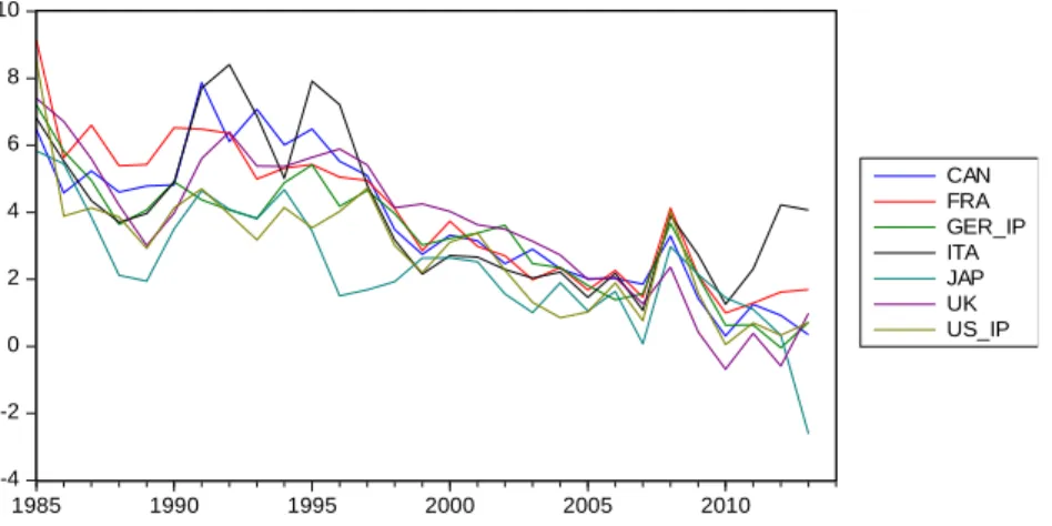
By that time, the introduction of the discussion ended up not being as relevant as Hansen might have thought, as the real interest rates rose sharply in the following years. More recently, in 2013, Larry Summers has brought back the discussion, reintroducing the concept as a “decline in the full employment real interest rate with low inflation, which can prevent the attainment of full employment indefinitely”. Summers focuses his analysis mainly on the period since 1985, which can be seen in Figure 1, and argues that “real interest rates in the industrial world will likely be lower than they have been historically”.
-4 -2 0 2 4 6 8 10 1985 1990 1995 2000 2005 2010 CAN FRA GER_IP ITA JAP UK US_IP
Figure 1. Real interest rates in the G7 countries since 1985 (Source: see section 2.2)
The main question brought by the Secular Stagnation discussion is: has the natural real interest rate declined recently to negative levels, compromising the convergence of the actual rate to the natural, in a context of near zero inflation? The main worry is that if the natural interest rate goes below zero, it may be impossible to clear the market for loanable funds, dooming the economy to a persistent unemployment. It has therefore been inferred (Krugman
4 2014) that macroeconomic policy as currently structured may have difficulty maintaining production at potential level.
The discussion has become particularly relevant again in recent years because of the real interest rates behavior since the Great Recession. As seen in Figure 1, these have generally declined since 2008, in a way that several influential economists (Summers 2014, Williams 2015, Hamilton et al. 2015, Krugman 2014, Gordon 2014, Blanchard et al. 2014, Crafts 2014, Glaeser 2014, Wolff 2014, Caballero et al. 2014, Jimeno et al. 2014) are now discussing whether this fall should be considered relevant in a long term perspective – hence Secular Stagnation – or if it might only be a phenomenon of cyclical nature.
The first possibility is addressed by John C. Williams (2015), who, based on his dataset from 1961, argues that “the fact that rates have been very low for close to seven years implies that standard statistical methods indicate that the fall in real rates is entirely due to a downward shift in trend” and “longer-term interest rates will be lower on average”, with “no sign of a return to a more normal trend”. In contrast, based on Forecasting and Structural Break tests in their data from 1800, Hamilton et al. (2015) are more skeptical of this new Secular Stagnation hypothesis, saying that there is “little evidence that the real interest rate will revert to a neutral value”.
In the context of this discussion, we intend to study real interest rates in a very long term perspective for nine countries, using data starting between 1703 (for the UK) and 1922 (for Japan), so that we may investigate if the Great Recession is a structural break in the series using different samples within our range, that is, enlarging the window successively, and look for previous episodes that may relate to or even have greater importance than the recent one. If so, the recent behavior of real rates might not be as relevant as Secular Stagnation hypothesis supporters suggest. We should notice that historical series, as the ones used for
5 this study, bring a new perspective to the discussion, as they are based on a larger information set, providing more evidence of the past and therefore more robustness to our analysis. Namely, our work addresses the following questions: Is the recent real rates decrease a significant break in our long-run series? What if we use shorter datasets? Will interest rates be permanently lower?
Therefore, to give reasoned answers to these questions, the data – explained in section 2.2 – is subject to two types of analysis: descriptive, in section 2.3, and empirical, in section 3. The empirical analysis includes testing for stationarity (3.1); testing for structural breaks (3.2); testing for a specific Great Recession structural break (3.3); comparing forecasts for the post-2007 period with what happened (3.4) and forecasting for future years up to 2020 (3.5).
2. Methodology 2.1. Background
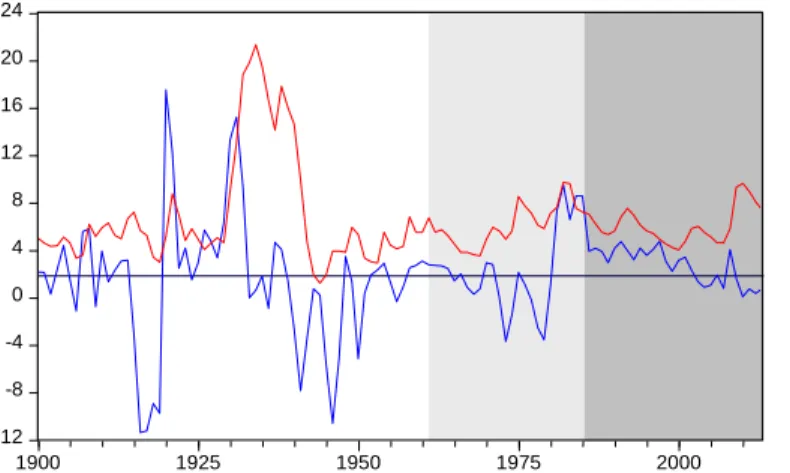
Figure 2 provides information for the U.S. real interest rate (in blue) and the U.S. unemployment rate (in red) for three different samples: 1985-2013, as in Summers (2014); 1961-2013, as done by Williams (2015); and 1900-2013. The real interest rate average for the larger sample is represented by the dark blue horizontal line.
-12 -8 -4 0 4 8 12 16 20 24 1900 1925 1950 1975 2000
Figure 2. U.S. Real Interest Rate (blue) and Unemployment Rate (red), 1900-2013
6 Looking only at the first sample, since 1985, we may say that the Great Recession (2007-2008) might be considered a break in the series. But moving on to the second one, since 1961, we see that the break does not look so relevant anymore, specially comparing to the increase around 1979, when the U.S. conducted aggressive monetary policy in response to the second petroleum shock, which can also be observed by the unemployment behavior at the time. So we decided to look into the greater picture: since 1900, there are lots of breaks like the one in 1979 or more obvious ones like the shift in rates after the Great Depression (1929-1933), which makes this post-Great Recession behavior look particularly different from past episodes.
After noticing that the relevance of the recent interest rates decrease changes depending on the time span considered, this brief graphical analysis was the motivation that led us to consider historical series for our study.
2.2. Data
As mentioned before, the collection of data for this study was a crucial point. We started by stating that the series would have an annual frequency and would start as early as we could find for each country. Consequently, the goal was to do an exhaustive gathering of data from many different sources, in order to construct long term time series of real interest rates for nine different countries: United Kingdom, United States, Canada, France, Germany, Japan, Netherlands, Italy and Portugal. These countries were chosen for being considered good representatives of the joint developed countries economic behavior, by including the Group of 7 (G7), plus Portugal and the Netherlands.
For that purpose, we have constructed the series one by one using data for:
Nominal interest rate: mainly the Long Term Government Bond Yield, which is usually the 10 Year Government Bond Yield. We have chosen this specific yield because it is
7 considered to be the most representative of general interest rates fluctuations and it represents financial markets reality in a broad perspective. In some cases, mostly concerning the earlier observations, the considered yield does not correspond to a Long Term Government Bond Yield as we are used to define it, but to a yield on British Consols, French Rentes, German Prussians, etc. These instruments are also bonds issued by the governments, but were issued as perpetual bonds redeemable at the option of the government. To test if these yields are representative of the general interest rate trend, we have computed the correlations between these rates and the respective long term government bond yields in the common observations, and the lower correlation we got was 76.6%.1 Therefore, we assume these rates to be representative of generic long term interest rates and adequate to be used in our long-run interest rate series.
Inflation rate: always based on the Consumer Price Index.
We have calculated the real interest rate for each country based on the following formula: 𝐫𝐭=
𝟏+𝐢𝐭
𝟏+𝛑𝐭+𝟏− 𝟏
, being rt the country’s ex-ante real interest rate at year t; it the country’s nominal interest
rate at year t and πt the country’s CPI inflation rate at year t.
This calculation is based on two assumptions:
i. The real rate is calculated being the nominal interest rate discounted by the expectations of next year’s inflation, πt+1e
ii. Perfect Forecast: the inflation forecast for next year is considered to be exactly correspondent to the value taken by inflation in that same year , πt+1e= πt+1
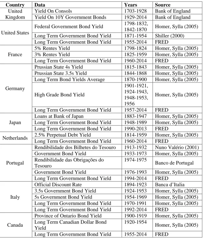
8 Therefore, for the calculation of rt, data for nominal interest rates and for inflation rates is
necessary. The data used to construct the series for the nominal rates, it, was taken from the
sources identified in Table 1. Graphs for these nine series can be found in Appendix II.
Table 1. Nominal interest rates data and respective sources
Country Data Years Source
United Kingdom
Yield On Consols 1703-1928 Bank of England
Yield On 10Y Government Bonds 1929-2014 Bank of England United States
Federal Government Bond Yield 1798-1832,
1842-1870 Homer, Sylla (2005) Long Term Government Bond Yield 1871-1954 Shiller (2000) Long Term Government Bond Yield 1955-2014 FRED
France
5% Rentes Yield 1798-1824 Homer, Sylla (2005)
3% Rentes Yield 1825-1959 Homer, Sylla (2005)
Long Term Government Bond Yield 1960-2014 FRED
Germany
Prussian State 4s Yield 1815-1843 Homer, Sylla (2005) Prussian State 3.5s Yield 1844-1868 Homer, Sylla (2005) Long Term Bond Yields Average 1870-1900 Homer, Sylla (2005) High Grade Bond Yield
1901-1921, 1924-1943, 1948-1953, 1956
Homer, Sylla (2005) Long Term Government Bond Yield 1957-2014 FRED
Japan
Loans at Bank of Japan 1883-1947 Homer, Sylla (2005) Long Term Government Bond Yield 1948-1989 Homer, Sylla (2005) Long Term Government Bond Yield 1990-2013 FRED
Netherlands 2.5% Perpetual Debt Yield 1814-1959 Homer, Sylla (2005) Long Term Government Bond Yield 1960-2014 FRED
Portugal
Rendibilidade dos Bilhetes do Tesouro 1913-1932 Nuno Valério (2001) Government Bond Yield 1933-1973 Homer, Sylla (2005) Rendibilidade das Obrigações do
Tesouro
1974-1975
Banco de Portugal Government Bond Yield 1976-1993 Homer, Sylla (2005) Long Term Government Bond Yield 1994-2014 FRED
Italy
Official Discount Rate 1894-1923 Banca d’Italia 3.5s Government Bond Yield 1924-1953 Homer, Sylla (2005) 5s Government Bond Yield 1954-1969 Homer, Sylla (2005) Long Term Government Bond Yield 1970-1991 Homer, Sylla (2005) Long Term Government Bond Yield 1992-2014 FRED
Canada
Province of Ontario Bond Yield 1900-1919 Homer, Sylla (2005) Long Term Canadian Dollar Bond
Yield
1920-1954
Homer, Sylla (2005) Long Term Government Bond Yield 1955-2014 FRED
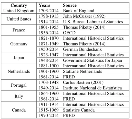
9 The different data sources for inflation rates, πt, are identified in Table 2. Again graphs for
the nine inflation series can be seen in Appendix III.
Table 2. Inflation data sources
Country Years Source
United Kingdom 1703-2014 Bank of England United States 1798-1913 John McCusker (1992)
1914-2014 U.S. Bureau Labour of Statistics France 1801-1955 Thomas Piketty (2014)
1956-2014 OECD Germany
1821-1870 International Historical Statistics 1871-1949 Thomas Piketty (2014)
1950-2014 German Bundesbank
Japan 1923-1947 International Historical Statistics 1948-2014 Government Statistics for Japan Netherlands
1881-1900 International Historical Statistics 1901-1960 StatLine Netherlands
1961-2014 FRED
Portugal 1703-1948 Carlos Bastien (2001)
1949-2014 Instituto Nacional de Estatística Italy 1864-1960 International Historical Statistics
1961-2014 FRED Canada
1911-1914 International Historical Statistics 1915-1969 Statistics Canada
1970-2014 FRED
In relation to the construction of the series, we had two issues:
Missing data: for some years we could not find any data. Those were all for the nominal interest rates series and it corresponded to the following years: from 1833 to 1841 for the United States; 1869, 1922, 1923, from 1943 to 1947 and from 1953 to 1955 for Germany. To solve this issue, we have interpolated our series in the said years, by using an algorithm called Cubic Hermite Spline Interpolation, which interpolates the missing values by using a third degree polynomial interpolation. The original real interest rates series for these countries – US and GER – were then replaced by series with the interpolated values – US_IP and GER_IP.
10
Outliers: a number of outliers can easily be found by analyzing graphically our real interest rates series. In order to formally identify these observations, we computed the RStudent statistic for every observation and proceeded to use a method of outlier detection based on this influence descriptive statistic. Tables with the highest RStudent values for each country are in Appendix IV. According to our criteria, which consisted in detecting every observation with an absolute value of RStudent higher than 6, this statistic has dictated the existence of the following outliers: the real rates for Germany in 1847 (56.74%) and 1919 (-56.72%); Italy in 1943 (-76.59%); Japan in 1945 (-83.08%) and the United Kingdom in 1711 (45.29%). All of these are observations that deviate from the other observations in a way that they might be generated by a different mechanism than the normal real interest rate trend, which is what we are aiming to study. Despite this, we should look at the historical context of these observations: all correspond to specific periods in the history of the countries when the inflation had an abrupt movement – because of post-war hyperinflation (Germany 1919; Italy 1943; Japan 1945) or very negative inflation stemming from economic crises (Germany 1847; United Kingdom 1711) – and the national government responded acting as a financial repressor, fixing the nominal interest rate. So, the real interest rate also moved abruptly in these years. Consequently, we may say that these specific outliers have reasonable explanations, which means that they should not be discarded. For these reasons, we proceeded to keep these observations in our series.
2.3. Descriptive Analysis
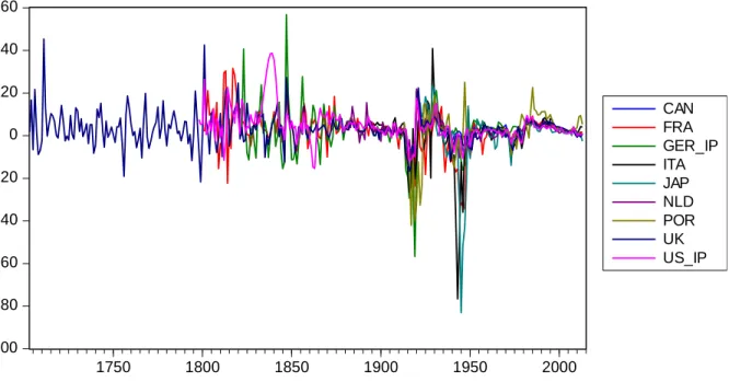
Having solved the issues with the data, we are now able to analyze the real interest rate series constructed for the nine countries. The graph of the entire series is displayed in Figure 3.
11 -100 -80 -60 -40 -20 0 20 40 60 1750 1800 1850 1900 1950 2000 CAN FRA GER_IP ITA JAP NLD POR UK US_IP Figure 3. Real interest rate series, all countries, all data (Source: see section 2.2)
To analyze the real interest rates historically, we also computed some descriptive statistics:
Table 3. Real interest rate series descriptive statistics
Country CAN FRA GER ITA JAP NLD POR UK US
First Year 1910 1801 1821 1894 1922 1880 1913 1703 1798 Observations 104 213 193 120 92 134 101 311 216 Average 2.61 1.87 2.39 0.10 -0.18 2.38 1.63 3.10 4.57 Median 2.63 2.68 3.38 2.72 1.92 2.38 2.70 2.62 3.41 Standard Deviation 4.67 9.39 9.83 12.42 13.42 4.85 10.69 7.41 7.79 Maximum 20.58 31.53 56.74 40.91 23.48 21.89 25.04 45.29 38.69 Maximum (year) 1920 1817 1847 1929 1929 1920 1947 1711 1839 Minimum -10.85 -34.44 -56.72 -76.59 -83.08 -12.65 -42.08 -21.73 -15.31 Minimum (Year) 1916 1947 1919 1943 1945 1917 1917 1799 1863 Amplitude 31.43 65.97 113.46 117.50 106.56 34.54 67.12 67.02 54.00
We can take several conclusions from Table 3. Firstly, if the series is level stationary (see section 3.1), the long-run trend for each country’s real interest rate might be measured by the respective series average, presented in the table. The volatility might be measured by the
12 standard deviation, being its nine countries average 8.94%. The countries that exhibit the higher volatility are Italy and Japan.
We can also infer from Figure 3 and Table 3 that the farthest points from the long-run tendency correspond to the periods of war or post-war, being the most obvious WWI (1914-1918) and WWII (1939-1945), which can clearly be seen as the two negative spikes in Figure 2. As stated in Table 3, these two events cover almost every country’s minimum real rates. This can easily be explained by the post-war hyperinflation phenomenon, mentioned earlier. Furthermore, considering only G7 countries and the years when all these have data (1922-2013), the correlations between the seven series vary from 43.61% (UK and Italy) to 87,23% (Canada and US), which is suggestive of interdependence.2
3. Empirical Analysis
In this section, we perform econometrical analysis on our long-run real interest rate series, in order to answer to our previously raised questions.
3.1. Stationarity
First of all, with the intent of better understanding the long-run behavior of our series, the first property to test for in each of our nine series is stationarity. Therefore, four different types of unit root tests – Augmented Dickey-Fuller (ADF), Phillips-Perron (PP), Kwiatkowski-Phillips-Schmidt-Shin (KPSS) and ADF with a breakpoint – were performed for each country series (when needed, the AR specification for each series is automatically generated according to the Schwarz criterion). The respective test results are displayed in Table 4, which reject the presence of unit root at a 1% significance level for all nine countries. All these tests are testing for level stationarity and were performed with drift and no trend.
13 This means that there is statistical evidence that the mean and the variance of each series do not change over time and each long-run real rate behavior does not follow any trend, cycle or random walk process.
Table 4. Results for the Unit Root Tests, all countries, all data
Test CAN FRA GER ITA JAP NLD POR UK US
ADF a 0.0000 0.0000 0.0000 0.0000 0.0046 0.0000 0.0001 0.0000 0.0000
PP b 0.0000 0.0000 0.0000 0.0000 0.0034 0.0000 0.0000 0.0000 0.0000
KPSS c 0.0985 0.4929 0.0958 0.1210 0.1269 0.1199 0.4784 0.4723 0.6888
ADF w/ Break d <0.01 <0.01 <0.01 <0.01 <0.01 <0.01 <0.01 <0.01 <0.01
a: Mac-Kinnon (1996) one-sided p-value; Null Hypothesis: the series has a unit root b: Mac-Kinnon (1996) one-sided p-value; Null Hypothesis: the series has a unit root c: KPSS test statistic (1% critical value: 0.739); Null Hypothesis: the series is stationary d: Vogelsang (1993) asymptotic one-sided p-value; Null Hypothesis: the series has a unit root
Having these conclusions, modeling and forecasting our series will provide consistent and reliable results. Also, knowing that all series are mean-reverting processes – the expectation is for each series to return to its mean at some point – and comparing the respective averages to the most recent values, the expectation is for rates to go up at some point in the future, as most of them (with the exceptions of Italy and Portugal) are currently below the average.
3.2. Structural Breaks
Our main focus is to ascertain whether the recent decline in rates is a significant break in each country’s series. To achieve that, we performed Bai-Perron tests of 1 to M globally determined breaks – with a maximum of 5 possible breaks –, using three different datasets:
a) Long-run: All observations gathered (CAN 1910; FRA 1801; GER 1821; ITA 1893; JAP 1922; NLD 1880; POR 1913; UK 1703; US 1798);
b) Medium-run: Every country with data from 1922; c) Short-run: Every country with data from 1976.
The Bai-Perron test results for each country, considering a 5% significance level, are summarized in Table 5 for the three datasets.
14
Table 5. Results for the Bai-Perron Tests, all countries, three different datasets
Country Significant Breaks (All Data) Significant Breaks (1922-2013) Significant Breaks (1976-2013)
Canada 1925, 1940, 1955, 1982, 1998 1935, 1952, 1965, 1981, 1998 1981, 1986, 1991, 1998, 2009 France 1833, 1875, 1914, 1952, 1983 1936, 1949, 1962, 1981, 1999 1981, 1993, 1998, 2003, 2009
Germany No breaks No breaks 1981, 1987, 1998, 2003, 2009
Italy No breaks No breaks 1981, 1991, 1997, 2002, 2008
Japan 1936, 1949, 1964, 1977, 1996 1936, 1949, 1964, 1977, 1996 1981, 1987, 1996, 2002, 2009 Netherlands No breaks 1936, 1951, 1964, 1977, 1998 1981, 1987, 1993, 1998, 2009 Portugal 1928, 1947, 1964, 1979, 1997 1939, 1952, 1970, 1984, 1997 1984, 1989, 1997, 2003, 2009 United Kingdom 1895 1936, 1952, 1968, 1981, 2001 1981, 1987, 1998, 2004, 2009 United States 1843, 1875, 1908, 1940, 1981 No breaks 1981, 1987, 1998, 2003, 2009
Considering only the long-run dataset, we have constructed graphs with each series and the correspondent significant breaks, which are presented in Appendix VI.
We can take several conclusions from the results presented in Table 5 and from the above mentioned graphs, specially regarding the goals of our study:
i. Looking only at the results from dataset a), the first aspect to notice is the absence of any period even remotely close to the Great Recession as a significant break. The most recent break is actually 1998, in Canada.
ii. The second, and most important of all, is the relevance of having different results when considering datasets a) and c): in every test considering c), either 2008 or 2009 is a significant break, which obviously corresponds to the Great Recession. This means that different perspectives lead to different conclusions.
iii. Also, we only need to consider our medium-run data – dataset b) –, to obtain interesting results: the most recent significant break obtained is 2001, in the United Kingdom, still distant from the Great Recession.
We may then conclude that the Great Recession only constitutes a significant break when considering a shorter time period for our analysis. This means that the recent decrease in real rates is not considered a significant movement when considering long or medium-run data.
15
3.3. Great Recession Break
With the intent to have more robust conclusions for our study, we decided to investigate whether the Great Recession specifically could be considered a break.
Firstly, in order to find the best specifications for modeling each of our country’s series, we decided to use the Box-Jenkins methodology. So, we started by obtaining each series’ correlogram to observe the behavior of sample autocorrelation and partial autocorrelation functions and therefore have some insights about the possible model. Afterwards, we applied Eviews add-in ARIMASEL for each series, which estimates every possible ARMA specification up to an ARMA (5,5) and calculates the Schwarz Criterion (BIC) for each model. The best model for each country corresponds to the one with the lowest BIC value and it is explicit in Table 6.
Having these specifications, we have adapted a simple concept suggested by Hamilton et al. (2015), which consisted in introducing in each model a possible shift in the level beginning at date t0 (in this case, t0=2007), named δ(t≥t0). δ is a dummy variable which takes the value 1 if year t is greater or equal to t0 and the value 0 for previous years. Then, we estimate the model – with the defined specifications – adding the newly introduced variable, to find out if it is statistically significant, that is, if there is a significant break in 2007.
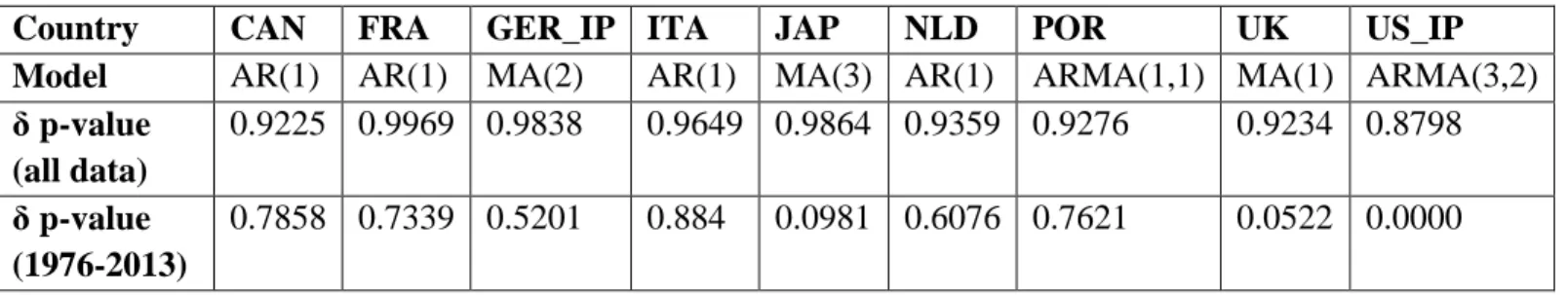
Table 6. Best model specification and δ significance, all data and 1976-2013
Country CAN FRA GER_IP ITA JAP NLD POR UK US_IP
Model AR(1) AR(1) MA(2) AR(1) MA(3) AR(1) ARMA(1,1) MA(1) ARMA(3,2)
δ p-value (all data) 0.9225 0.9969 0.9838 0.9649 0.9864 0.9359 0.9276 0.9234 0.8798 δ p-value (1976-2013) 0.7858 0.7339 0.5201 0.884 0.0981 0.6076 0.7621 0.0522 0.0000
The main conclusion from these results is that, for every country, using all data, the dummy introduced is not statistically significant – even at an 85% level –, which suggests again that
16 the Great Recession does not consist of a significant break with this perspective. However, if we consider the shorter dataset, 1976-2013, performing the same method now yields δ as significant at a 10% level for the UK, the US and Japan, thus showing one more time that the Great Recession may only be a significant break when considering short-run data.
3.4. Forecasting vs. Reality
For another way of measuring how much of a break in real interest rates series was the Great Recession, we have decided to consider a subsample of all data until 2006 and forecast the observations from 2007 to 2013 for each country, and then compare these forecasts with the actual values. Some conclusions might be taken from this comparison: the closer the forecasts get to what happened after 2007, the least of a break exists that year.
We have used what is called an Automatic ARIMA Forecasting, which chooses a model that minimizes the Schwarz Criterion for the subsample considered and produces forecasts for the following 7 years, which we have called F_BIC. These forecasts and respective comparisons with the real values are represented graphically in Appendix VII.
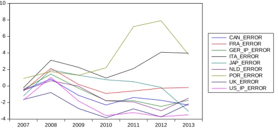
To summarize the forecasting accuracy, we computed the forecast error, which is the difference between the actual real interest rates and F_BIC, for every country between 2007 and 2013, which is represented in Figure 4. These differences tell us that, for this period, the real rates were generally lower than the forecasts (with the exceptions of Portugal and Italy), meaning that the expectation was not necessarily for interest rates to fall as they did.
17 -4 -2 0 2 4 6 8 10 2007 2008 2009 2010 2011 2012 2013 CAN_ERROR FRA_ERROR GER_IP_ERROR ITA_ERROR JAP_ERROR NLD_ERROR POR_ERROR UK_ERROR US_IP_ERROR
Figure 4. Difference between Reality and Forecasts, all countries, 2007-2013
In order to measure how much of the decrease was expected, we computed the Mean Absolute Percent Error (MAPE) for each country, which is provided in Appendix VIII. It indicates that the country with the highest forecasting accuracy was France (62%) and the one with the lowest was the UK (10%). The average forecast accuracy was 30%, which reflects that the decline was not expected, even if it is not a break in the series.
3.5. Forecasts up to 2020
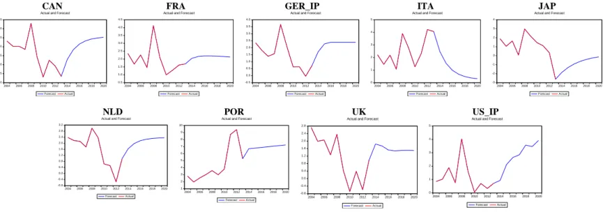
Using the same method as in the previous section, but considering the whole sample 1703-2013, forecasts for future years 2014-2020 were produced, with the intent of having a new insight on whether low real interest rates are going to persist or not.
These forecasts are represented in Figure 5. We can clearly see that eight of the nine countries in our sample have higher forecasted rates in 2020 than the present values. This constitutes another piece of evidence for the argument that real interest rates will not decline below the average level observed in the past. The only exception to the dominant pattern is Italy, which might be explained by the current high value of the yields on Italian Government Bonds, stemming mainly from the country’s level of public debt.
18 CAN 0.0 0.5 1.0 1.5 2.0 2.5 3.0 3.5 2004 2006 2008 2010 2012 2014 2016 2018 2020 Forecast Actual
Actual and Forecast FRA
0.5 1.0 1.5 2.0 2.5 3.0 3.5 4.0 4.5 2004 2006 2008 2010 2012 2014 2016 2018 2020 Forecast Actual
Actual and Forecast GER_IP
-0.5 0.0 0.5 1.0 1.5 2.0 2.5 3.0 3.5 4.0 2004 2006 2008 2010 2012 2014 2016 2018 2020 Forecast Actual
Actual and Forecast ITA
0 1 2 3 4 5 2004 2006 2008 2010 2012 2014 2016 2018 2020 Forecast Actual
Actual and Forecast JAP
-3 -2 -1 0 1 2 3 4 2004 2006 2008 2010 2012 2014 2016 2018 2020 Forecast Actual
Actual and Forecast
NLD -0.8 -0.4 0.0 0.4 0.8 1.2 1.6 2.0 2.4 2.8 3.2 2004 2006 2008 2010 2012 2014 2016 2018 2020 Forecast Actual Actual and Forecast
POR 1 2 3 4 5 6 7 8 9 10 2004 2006 2008 2010 2012 2014 2016 2018 2020 Forecast Actual
Actual and Forecast
UK -0.8 -0.4 0.0 0.4 0.8 1.2 1.6 2.0 2.4 2.8 2004 2006 2008 2010 2012 2014 2016 2018 2020 Forecast Actual
Actual and Forecast
US_IP 0 1 2 3 4 5 2004 2006 2008 2010 2012 2014 2016 2018 2020 Forecast Actual
Actual and Forecast
Figure 5. Graphs for 2014-2020 Forecasts, all countries
5. Conclusion
In order to take conclusions from our study, we should look back into the questions raised at the beginning of our discussion and try to give answers based on our results.
First of all, the main and most relevant conclusion we may take is that, looking at the data in a long-run perspective, since 1703, there is no statistically significant structural break corresponding to the Great Recession. Even looking since 1922, there is no break in the series at that time. There is a significant break only if we look since 1976.
This means that, if we take a long-run perspective as the one adopted in this study, the Great Recession is not a structural break in real interest rate series and it is, most likely, only a cyclical episode. It becomes clear that different conclusions might be taken from different information sets; therefore, gathering data as early as 1703 was a crucial point for our work. Using the largest information set possible should be a priority, because it gives us more robust results and, therefore, more well-founded conclusions. In our case, the conclusion of the recent decrease in rates not being a structural break, looking at the longer series, should be a result with superior relevance to the result based in the short-run series.
19 These results may be seen as challenging the new Secular Stagnation hypothesis (Summers 2013), bringing a new perspective – mainly based on historical data – to the discussion. As it was observed, the recent behavior is not a permanent stagnation in the real rates series; it looks more like one more episode with no statistical significance in the long-run.
Limitations to our work include the fact that we did not relate our analysis of breaks with the real interest rate determinants (Afonso and Rault 2011, Blanchard et al. 2014). The natural interest rate concept is also absent, for not being practically measurable. Moreover, the current economic paradigm may not be directly comparable to other historical periods in our long-run dataset, as distinct centuries have completely different contexts. Our statistical analysis is also not perfectly accurate in relation to reality, as it is based on many assumptions. Assessing the sensitivity of the results obtained from our statistical techniques when gradually changing the time span would be a useful path for further research.
In relation to monetary policy: even if a lot of interest rates defined by central banks are, at the moment, zero or near zero, and therefore we are facing a zero lower bound, this will most likely not be a permanent problem, as it has been suggested by some authors (Williams 2015, Blanchard et al. 2014). The mean-reverting property of our series tells us that the tendency is for rates to go back to their average, which means, today, to increase at some point in the near future. This point is also reiterated by our forecasts up to 2020.
In sum, our results suggest that the recent impact is not permanent and therefore rates will eventually return to more normal levels, as we are starting to see, for instance, in the United States – the Fed has increased the Federal Funds Rate in December.
20
References
Afonso, A. and Rault, C. 2011. “Long-run determinants of sovereign yields” Economics
Bulletin, 31(1): 367-374.
Armstrong, A., Caselli, F., Chadha, J. and den Haan, W. 2014. “Monetary policy at the
zero lower bound”, VoxEU. Available at: http://www.voxeu.org/article/macroprudential-policy-survey-uk-based-macroeconomists.
Bastien, C. 2001. “Preços e Salários” In Estatísticas Históricas Portuguesas, ed. Nuno
Valério, 615-655. Lisboa: Instituto Nacional de Estatística.
Blanchard, O., Furceri, D. and Pescatori, A. 2014. “A prolonged period of low real
interest rates?” In Secular Stagnation: Facts, Causes and Cures, ed. Coen Teulings and Richard Baldwin, 101-110. London: CEPR Press.
Caballero, R. J. and Farhi, E. 2014. “On the role of safe asset shortages in secular
stagnation” In Secular Stagnation: Facts, Causes and Cures, ed. Coen Teulings and Richard Baldwin, 111-122. London: CEPR Press.
Crafts, N. 2014. “Secular stagnation: US hypochondria, European disease?” In Secular
Stagnation: Facts, Causes and Cures, ed. Coen Teulings and Richard Baldwin, 91-98.
London: CEPR Press.
Gordon, R. J. 2014. “The turtle’s progress: Secular Stagnation meets the headwinds” In
Secular Stagnation: Facts, Causes and Cures, ed. Coen Teulings and Richard Baldwin,
47-60. London: CEPR Press.
Glaeser, E. L. 2014. “Secular joblessness” In Secular Stagnation: Facts, Causes and
Cures, ed. Coen Teulings and Richard Baldwin, 69-80. London: CEPR Press.
Hamilton, J. D., Harris, E. S., Hatzius, J. and West, K. D. 2015. “The equilibrium real
funds rate: Past, present, and future”, Hutchins Center on Fiscal & Monetary Policy at Brookings, Working Paper 16, October 30.
Hansen, A. 1939. “Economic Progress and Declining Population Growth” American
Economic Review, 29(1): 1–15.
Homer, S. and Sylla, R. 2005. A History of Interest Rates. New Jersey: John Wiley &
Sons.
Jimeno, J. F., Smets, F. and Yiangou, J. 2014. “Secular stagnation: A view from the
Eurozone” In Secular Stagnation: Facts, Causes and Cures, ed. Coen Teulings and Richard Baldwin, 153-164. London: CEPR Press.
Krugman, P. 2014. “Four observations on secular stagnation” In Secular Stagnation:
Facts, Causes and Cures, ed. Coen Teulings and Richard Baldwin, 61-68. London: CEPR
21
McCusker, J. J. 1992. How Much Is That in Real Money? A Historical Price Index for
Use as a Deflator of Money Values in the Economy of the United States. Worcester, MA:
American Antiquarian Society.
Piketty, T. 2014. Capital in the Twenty-First Century. Cambridge, MS: Harvard University
Press.
Shiller, R. J. 2000. Irrational Exuberance. New Jersey: Princeton University Press.
Summers, L. H. 2013. “Crises Yesterday and Today”, speech at the 14th Jacques Polak
Annual Research Conference. Washington, DC, 7 November.
Summers, L. H. 2014. “Reflections on the ‘New Secular Stagnation Hypothesis’” In
Secular Stagnation: Facts, Causes and Cures, ed. Coen Teulings and Richard Baldwin,
27-38. London: CEPR Press.
Valério, N. 2001. O Escudo: A Unidade Monetária Portuguesa 1911-2001. Lisboa, Banco
de Portugal.
Williams, J. C. 2015. “Will interest rates be permanently lower?”, VoxEU. Available at:
http://www.voxeu.org/article/evidence-low-real-rates-will-persist.
Wolff, G. B. 2014. “Monetary policy cannot solve secular stagnation alone” In Secular
Stagnation: Facts, Causes and Cures, ed. Coen Teulings and Richard Baldwin, 143-150.
22
Appendix I. Correlations between different yields in common years
Country Years Yields Correlation
Canada 1920-1943 Province of Ontario, Long Term Canadian Dollar Bonds 0.984919 1955-1989 Long Term Canadian Dollar Bonds, Long Term GB 0.998887
France 1825-1852 5% Rentes, 3% Rentes 0.937455
1960-1969 3% Rentes, Long Term GB 0.88593
Germany
1853-1868 Prussian 4s, Prussian 3.5s 0.894552
1870-1883 Prussian 4s, Long Term Bond 0.876101
1957-1989 High Grade Bond, Long Term GB 0.975877
Italy 1924-1949 Official Discount Rate, 3.5s GB 0.766389
1970-1998 Official Discount Rate, Long Term GB 0.874137 Japan 1930-1960 Loans Bank of Japan, Long Term GB 0.920051 1966-1989 Loans Bank of Japan, Long Term GB 0.894668
Netherlands 1959-1975 Perpetual Debt, Long Term GB 0.98762
Portugal 1993-1998 Bilhetes do Tesouro, Long Term GB 0.930705
United Kingdom 1929-2014 Consols, 10y GB 0.983502
United States 1871-1899 Federal GB, Long Term GB 0.775833
Appendix II. Nominal Rate Series Graphs
0 4 8 12 16 1750 1800 1850 1900 1950 2000 CAN 0 10 20 30 40 1750 1800 1850 1900 1950 2000 FRA 0 2 4 6 8 10 12 1750 1800 1850 1900 1950 2000 GER 0 5 10 15 20 25 1750 1800 1850 1900 1950 2000 ITA 0 2 4 6 8 10 1750 1800 1850 1900 1950 2000 JAP 0 2 4 6 8 10 12 1750 1800 1850 1900 1950 2000 NLD 0 5 10 15 20 25 30 1750 1800 1850 1900 1950 2000 POR 0 4 8 12 16 1750 1800 1850 1900 1950 2000 UK 0 4 8 12 16 1750 1800 1850 1900 1950 2000 US
23
Appendix III. Inflation Rate Series Graphs
-20 -10 0 10 20 1750 1800 1850 1900 1950 2000 CAN -20 0 20 40 60 1750 1800 1850 1900 1950 2000 FRA -150 -100 -50 0 50 100 150 1750 1800 1850 1900 1950 2000 GER -100 0 100 200 300 400 1750 1800 1850 1900 1950 2000 ITA -200 0 200 400 600 1750 1800 1850 1900 1950 2000 JAP -20 -10 0 10 20 1750 1800 1850 1900 1950 2000 NLD -20 0 20 40 60 80 100 1750 1800 1850 1900 1950 2000 POR -40 -20 0 20 40 1750 1800 1850 1900 1950 2000 UK -20 -10 0 10 20 30 1750 1800 1850 1900 1950 2000 US
Appendix IV. Highest RStudent values for each country
CAN FRA GER_IP ITA JAP NLD POR UK US_IP
Year * Year * Year * Year * Year * Year * Year * Year * Year *
1920 4.16 1947 4.01 1919 6.68 1943 7.50 1945 8.14 1920 4.29 1917 4.49 1711 6.02 1839 4.59 1930 3.04 1945 3.78 1847 6.03 1944 4.10 1946 4.17 1921 3.37 1919 4.17 1801 5.57 1838 4.54 1916 3.00 1946 3.60 1823 4.05 1929 3.45 1947 3.41 1917 3.22 1922 3.37 1799 3.41 1840 4.16 1947 2.91 1944 3.55 1916 3.33 1942 3.19 1944 2.25 1892 2.77 1920 3.36 1847 3.31 1837 4.10 1921 2.77 1817 3.24 1918 2.67 1946 3.01 1929 1.79 1944 2.70 1923 2.37 1756 3.03 1836 3.41
* RStudent absolute value
Appendix V. Correlation Matrix considering all countries in 1922-2013
Corr. CAN FRA GER_IP ITA JAP NLD POR UK US_IP
CAN 1 0.609 0.717 0.399 0.506 0.668 0.177 0.770 0.872 FRA / 1 0.673 0.623 0.685 0.563 0.292 0.520 0.637 GER_IP / / 1 0.453 0.769 0.541 0.114 0.495 0.731 ITA / / / 1 0.466 0.453 0.309 0.436 0.475 JAP / / / / 1 0.519 0.137 0.466 0.542 NLD / / / / / 1 0.336 0.772 0.622 POR / / / / / / 1 0.201 0.344 UK / / / / / / / 1 0.703 US_IP / / / / / / / / 1
24
Appendix VI. Real Rate Series Graphs with Breaks (from Bai-Perron tests)
CAN -20 -10 0 10 20 -20 -10 0 10 20 30 1910 1920 1930 1940 1950 1960 1970 1980 1990 2000 2010
Residual Actual Fitted
FRA -40 -20 0 20 40 -40 -20 0 20 40 1825 1850 1875 1900 1925 1950 1975 2000
Residual Actual Fitted
GER_IP -80 -40 0 40 80 -60 -40 -20 0 20 40 60 1825 1850 1875 1900 1925 1950 1975 2000
Residual Actual Fitted
ITA -80 -40 0 40 80 -80 -40 0 40 80 1900 1925 1950 1975 2000
Residual Actual Fitted
JAP -80 -60 -40 -20 0 20 40 -100 -80 -60 -40 -20 0 20 40 1930 1940 1950 1960 1970 1980 1990 2000 2010
Residual Actual Fitted
NLD -20 -10 0 10 20 -20 -10 0 10 20 30 1900 1925 1950 1975 2000
Residual Actual Fitted
POR -40 -20 0 20 40 -60 -40 -20 0 20 40 1920 1930 1940 1950 1960 1970 1980 1990 2000 2010
Residual Actual Fitted
UK -40 -20 0 20 40 60 -40 -20 0 20 40 60 1750 1800 1850 1900 1950 2000
Residual Actual Fitted
US_IP -30 -20 -10 0 10 20 30 -20 -10 0 10 20 30 40 1800 1825 1850 1875 1900 1925 1950 1975 2000
25
Appendix VII. Forecasting vs. Reality Graphs, 2007-2013
CAN 0 1 2 3 4 5 6 1998 2000 2002 2004 2006 2008 2010 2012 Forecast Actual Actual and Forecast
FRA 0 1 2 3 4 5 1998 2000 2002 2004 2006 2008 2010 2012 Forecast Actual
Actual and Forecast
GER_IP -1 0 1 2 3 4 5 1998 2000 2002 2004 2006 2008 2010 2012 Forecast Actual Actual and Forecast
ITA 0 1 2 3 4 5 1998 2000 2002 2004 2006 2008 2010 2012 Forecast Actual Actual and Forecast
JAP -3 -2 -1 0 1 2 3 4 1998 2000 2002 2004 2006 2008 2010 2012 Forecast Actual Actual and Forecast
NLD -1 0 1 2 3 4 1998 2000 2002 2004 2006 2008 2010 2012 Forecast Actual Actual and Forecast
POR 1 2 3 4 5 6 7 8 9 10 1998 2000 2002 2004 2006 2008 2010 2012 Forecast Actual Actual and Forecast
UK -1 0 1 2 3 4 5 6 1998 2000 2002 2004 2006 2008 2010 2012 Forecast Actual Actual and Forecast
US_IP 0 1 2 3 4 5 1998 2000 2002 2004 2006 2008 2010 2012 Forecast Actual Actual and Forecast
Appendix VIII. Mean Absolute Percentage Error, 2007-2013
Country CAN FRA GER ITA JAP NLD POR UK US