http://www.uem.br/acta ISSN printed: 1679-9275 ISSN on-line: 1807-8621
Doi: 10.4025/actasciagron.v39i3.32564
Methodology for rainwater reservoir dimensioning: a probabilistic
approach
Wagner Wolff1*, Sergio Nascimento Duarte1, Olívio José Soccol2, Lineu Neiva Rodrigues3 and Rafael Dreux Miranda Fernandes4
1
Departamento de Engenharia de Biossistemas, Escola Superior de Agricultura “Luiz de Queiroz”, Universidade de São Paulo, Avenida Pádua Dias, 11, 13418-900, Piracicaba, São Paulo, Brazil. 2
Laboratório de Irrigação e Drenagem, Centro Agro Veterinário de Ciências, Universidade do Estado de Santa Catarina, Lages, Santa Catarina, Brazil. 3
Empresa Brasileira de Pesquisa Agropecuária, Embrapa Cerrados, Brasília, Distrito Federal; Brazil. 4
Departamento de Cristalografia, Mineralogia e Química Agrícola, Universidad de Sevilla, Sevilha, Espanha. *Author for correspondence: E-mail: wwolff@usp.br
ABSTRACT. The aim of this study was to propose a new methodology for reservoir rainwater dimensioning based on probabilistic modeling. Eucalyptus seedlings grown in a greenhouse were used to obtain a hypothetical water demand. Meteorological data were used to estimate the demand (evapotranspiration) and offer (rainfall over the greenhouse coverage). The probability distribution of Wakeby presented the best fit for the rainfall data; therefore, a Wakeby distribution was used to model the flow-duration curve of the greenhouse coverage. For a payback period (T) of 10 years of surplus water demand and water supply deficit, a reservoir with 13.60 m³ was obtained. The proposed methodology combined the simultaneous occurrence of the events to enable the scaling out of a reservoir with high safety to supply the required demand (T = 100 years) and therefore enables a lower cost of deployment compared to each approach separately (T = 10 years).
Keywords: Wakeby distribution, irrigation, sustainable practices, water resources.
Metodologia para dimensionamento de reservatórios de captação de águas pluviais: uma
abordagem probabilística
RESUMO. O objetivo deste trabalho foi apresentar uma nova metodologia para dimensionamento de RCAPs com base em modelagem probabilística. Para determinar uma demanda hídrica hipotética, utilizou-se a cultura do Eucalipto cultivada em casa de vegetação (CV). Dados meteorológicos foram utilizados para estimar, demanda (evapotranspiração) e oferta (precipitação incidente na cobertura da CV). A distribuição de probabilidade de Wakeby apresentou o melhor ajuste aos dados de precipitação; portanto, foi utilizada para modelar a curva de permanência do escoamento gerado na cobertura da CV e, assim, determinar o volume de um RCAP para suprir a demanda da cultura. Para um tempo de retorno (T) de 10 anos de excedente hídrico da demanda e de déficit hídrico da oferta, obteve-se um volume do RCAP de 13,60 m³. Assim, pela combinação de ocorrência simultânea dos eventos, pode-se concluir que a metodologia proposta permite dimensionar reservatórios com alta segurança de atendimento da demanda (T = 100 anos) e, consequentemente, com menor custo de implantação, comparado com as abordagens separadas (T = 10 anos).
Palavras-chave: distribuição de Wakeby, irrigação, práticas sustentáveis, recursos hídricos.
Introduction
Water scarcity problems, which are caused by raising demands and poor fountain conservation, represent one of the primary difficulties faced by agencies responsible for the administration of water resources (UN–Water, 2014).
When access to water resources is limited, reservoirs for rainwater harvesting (RRWH) become important water supply alternatives. Moments of limited water resources can result during a low qualitative and quantitative availability of fountains, as
observed in the water crisis in the Northeast and Southeast of Brazil in 2012/2014. This can also occur when there is excessive demand by the users of hydrographic basins, such as the basins of the rivers Piracicaba, Capivari and Jundiaí (PCJ) (Agência Nacional de Águas [ANA], 2014). Reservoirs for rainwater harvesting only require an area to harvest the incident rainwater to reserve the generated outflow.
projected an RRWH for uses considered low demand, such as cleaning vehicles, sidewalks and garden watering. These authors showed that for these uses, the RRWH was an excellent solution that ensured high system efficiency (higher than 90%). Akter and Ahmed (2015) evaluated the potential of implementing of RRWHs in an urban community in the city of Chittagong in Bangladesh. These authors used a multiple-criteria decision analysis together with a hydrological model to determine the potential superficial runoff to be stored. RRWHs can generate a damping of the wave and flood of approximately 326%, as well as supplementing the urban water supply system with 20 liters per day per person.
In rural regions, the challenge is to ensure an adequate and regular food supply for an increasing population with the lowest possible amount of water. Irrigation plays an important role in food production (Biazin, Sterk, Temesgen, Abdulkedir, & Stroosnijder, 2012; Carvajal, Agüera, & Sánchez-Hermosilla, 2014; Unami, Mohawesh, Sharifi, Takeuchi, & Fujihara, 2015); however, irrigation is the primary user of water resources and is responsible for approximately 70% of the withdrawn flow rates (UN-Water, 2014). Therefore, the study and development of techniques that enhance water availability are increasingly important. In this sense, the use of RRWHs represents a notable possibility for irrigation.
According to the methods of RRWH dimensioning used, the Associação Brasileira de Normas Técnicas (ABNT – Brazilian association of technical standards) published the NBR 15527 in 2007, which addresses the rainwater harnessing for non-potable purposes in urban areas (Associação Brasileira de Normas Técnicas [ABNT], 2007). This norm presents, in its attachment, six methods for the dimensioning of the volume of the reservoir used to store rainwater. The Rippl method, also known as Mass Curve Analysis, is the most cited in literature and has an easy application; however, this method can lead to oversizing when it is applied to dimensioning large reservoirs (Amorim & Pereira, 2008). The Simulation Method consists of determining the volume of the reservoir and verifying the percentage of consumption required. Finally, the Azevedo Neto, German Practical, British Practical and Australian Practical are approximated methods that are based on known empiric relations.
None of the methods proposed by the NBR 15527 fits any scenario; the values diverge considerately, approximately 100 m³ of difference between the most conservative to the higher ranges.
Thus, the draftsman must determine which method best fits a given situation (Amorim & Pereira, 2008; Lopes, Silva Junior, & Miranda, 2015). To avoid subjective dimensioning, (which often results in under- or over-estimations) and to efficiently attribute a water supply to the reservoir in answering water demand, it is important to consider the stochastic characteristics of rainfall via probabilistic modeling (Youn, Chung, Kang, & Sung, 2012; Morales-Pinzón, Rieradevall, Gasol, & Gabarrell, 2015; Unami et al., 2015). In Brazil, the recommended methodologies for the dimensioning of RRWHs do not yet consider the current state of the art. The implementation of a new methodology that involves probabilistic questions of RRWH dimensioning in Brazilian conditions is warranted.
The objective of this work was to present a new methodology for the dimensioning of rainwater harvesting reservoirs using probabilistic models.
Material and methods
The water demand of the eucalyptus crop grown under greenhouse located in Piracicaba-SP (longitude 47° 38’ 56” W and latitude 22° 43' 30” S) was used to test the proposed methodology.
According to the climatic classification of Rubel and Kottek (2010), the climate type Cwa prevails in the region: a subtropical humid climate with dry winters and hot summers.
The greenhouse had the following characteristics: (I) a shallow bowed ceiling with a plastic cover and a superficial runoff coefficient (C) equal to 0.90 (Li, Xie, & Yan, 2004), (ii) a coverage area equal to 100 m², (iii) an inner area equal to 100 m², (iv) irrigation by micro aspersion with an application efficiency (ef) of 90% (Frizzone, Freitas,
Rezende, & Faria, 2012), (v) a mean daily irrigation time (tirri) of 1.5h, and (vi) eucalyptus seedlings
arranged in plastic tubes.
Regarding the meteorological data, monthly average historical series were used from the conventional meteorological station administered by Escola Superior de Agricultura “Luiz de Queiroz” (ESALQ/USP), for the maximum, average and minimum temperature and precipitation for the period from 1917 to 2015. The meteorological station is located approximately 1.2 km from the greenhouse. Meteorological data mining was performed using Microsoft Excel 2010 with EasyFit 5.5, which was made available with the Visual Basic programming language.
empiric equation of Hargreaves-Samani (Hargreaves, 1994), as expressed by Equation 1:
ET0=0,0023 Q0 (TM-Tm)0,5 (T+17.8) (1)
In which: Q0 is the theoretical value of solar
radiation (mm day-1), T
M is the maximum
temperature (°C), Tm is the minimum temperature
(°C), and T is the average temperature (°C).
Q0 is calculated according to the latitude of the
area and the day of the year. For this calculation, the methodology proposed by Angelocci, Sentelhas, and Pereira (2002) was used. The author also presents a comparison between ET0 values as estimated by
Penman-Monteith FAO-56 (Allen, Pereira, Raes, & Smith, 1998) and Hargreaves-Samani (Hargreaves, 1994) and emphasizes that the difference between the ET0 estimated using both methodologies for the
city of Piracicaba, São Paulo State, is not significant. ET0 was then multiplied by the eucalyptus crop
coefficient (kc) regarding its initial physiological stage (equal to 0.70, Tatagiba et al., 2015) to obtain crop evapotranspiration (ETC).
The area to be irrigated by micro-aspersion inside the greenhouse represents 70% of the total area (i.e., 70 m²); this was used to determine the volume of water necessary to irrigate the crop for one month (Equation 2):
Virri=ETc Ai 0.001 (2)
In which: Virri is the volume to be stored (m³),
ETC is the monthly crop evapotranspiration (mm
month-1), and A
i is the irrigated area (m2).
The monthly volumes estimated to supply the crop water demand were used to determine the highest volume for each year of the data series (from 1917 to 2015). The maximum values were then arranged in decreasing order to define the probability of the demanded volume to be equaled or exceeded. The plotting positions of Kimball (Naghettini & Pinto 2007) were expressed as follows (Equation 3):
Pi=n+1m (3)
In which: m is the order of decreasing data classification, n is the size of the sample, and Pi is the
probability of the equality of the event.
According to Keller and Bliesner (1990), localized irrigation systems using micro-aspersion have a lifespan of 10 years. Therefore, the demanded volume was chosen for a payback period (T) of 10 years.
Finally, Virri corresponded to a T of 10 years. The
demanded outflow (QD) was obtained in Equation
4.
QD=Veirri.10
ftirri (4)
In which: Virri.10 is the irrigation volume for T
equal to 10 years (m³), ef is the application
efficiency, tirri the irrigation time (h), and QD is the
demanded outflow (m³ month-1). Notably, it was
not necessary to adjust the water demand to a theoretic probability distribution when the payback period used was equal to 10 years in the interval of the used data series, which was equal to 98 years.
Three probability distributions were evaluated to model the monthly precipitation: (i) Normal, (ii) Gamma, and (iii) Wakeby.
The Normal distribution is a model of two parameters in which the function of accumulated distribution (FDC) and the function of probability density (FDP) are given in Equations 5 and 6, respectively.
F(x)= e
-12 x - μσ 2
σ√2π
x
-∞ dx
(5)
f(x)=e
-12x - μσ 2
σ√2π
(6)
In which: µ and σ are the parameters of the distribution of location and shape, respectively. The variable x can assume any value between the interval (- ∞, + ∞).
The Gamma distribution in its general shape has three parameters. The FDC and FDP of this distribution are defined in Equations 7 and 8, respectively.
F(x)=Γ(x-γ) βΓ(α)⁄ (α) (7)
f(x)=(x - γ)α-1
Γ(α) e(-(x - γ) β⁄ )
(8)
In which: α, β and γ are the distribution parameters of shape, scale and location, respectively,
Γ(α) is the Gamma function with α as its domain, and x assumes values in the interval of γ to + ∞.
is shown in Equation 9 (also known as a quantile function).
x(F)=
+αβ 1-(1-F)β -γδ 1-(1-F)-δ (9)
In which: ξ is the parameter of location, α/β and γ/δ
are predominantly related with the scale, β and δ are exponential parameters defining the shape of the respective function, and F is equal to P (X ≤ x); in other words, it is the probability of the occurrence of events smaller than or equal to x.
The following conditions must be present for Equation 9 to be valid: (i) β + δ > 0 or β = γ = δ = 0; (ii) if α = 0 then β = 0; (iii) if γ = 0 then δ = 0; (iv) γ
≥ 0; α + γ > 0 (Hosking & Wallis, 1997). Estimating the parameters of the distributions cited above was performed using the L Moment Method (L-MM) (Hosking & Wallis, 1997). However, using the Wakeby distribution, it was not possible to analytically determine the percentiles (F). Thus, the value of F, corresponding to the sample quantile, was estimated using the numeric method of Newton-Rhapson (Abramowitz & Stegun, 1964).
The Anderson-Darling (AD) goodness of fit test was used to select the probability distribution that best fit the rainfall data (Anderson & Darling, 1954). This test is based on the difference between the cumulative probability functions, empiric FE(x), and theoretic
FT(x) of continuous random variables.
This was intended to give higher importance to the tails of the distribution, in which the higher (or lower) observations of the sample can alter the quality of the fit (Naghettini & Pinto, 2007). The Anderson-Darling (Equation 10):
A2 = - n - 1
n (2i-1)[lnF(xi+
n
i=1
+ ln(1-F(x ))] (10)
In which: {X(1), X(2), X(n) …} represent the
observations arranged in decreasing order and n represents the sample size. The tested hypotheses indicate that H0 data follow a specified distribution; H1 data do not follow a specified distribution.
To model the rainwater harvesting reservoir dimensioning, the monthly rainfall empirical flow-duration curve was elaborated by arranging it in decreasing order and by assigning probabilities of an event to be equaled or exceeded, as determined by Equation 3.
The site where the study was performed presents dry winters with the possibility of two months without raining. It was thus necessary to use the
theorem of total probability proposed by Hann (1977), Equation 11.
Pi= Pi* P(i>0) (11)
In which Pi* corresponds to the duration of the
rainfall sample different from zero, P(i>0) refers to the probability of a rainfall P, and Pi is the final
duration. In Equation 11, the term P(i>0) works as a correction factor for the durations related to the rainfall samples different from zero. Following this, the monthly rainfall (mm month-1) that falls in the
(10) area of the greenhouse ceiling was transformed in monthly flow (m3 month-1) using Equation 12.
QP= i1000PC A (12)
In which: ip is the intensity of the monthly
rainfall (mm month-1) modeled by a probability
distribution, C is the superficial runoff coefficient of the greenhouse cover, A is the area of the coverage (m2), and QP is the runoff generated by the rain that
falls on the greenhouse coverage (m3 month-1)
associated with a period of permanence.
Finally, to estimate the volume of the reservoir needed by the eucalyptus seedlings, the boundary between the areas was delineated by a horizontal line, representing the demanded outflow considered constant (Qd) and the area covered by the duration
curve, both calculated from the insertion point of the corresponding lines (Figure 1). The value of the reservoir’s volume (Vr) is given in Equation 13 as
follows.
Vr= ( -p) - pQd Qd- QpdpQd τ-p
pQd
∆T (13)
Therefore, substituting Equation 9 into equation 12 and adding the value of the respective parameters and variables, an equation was obtained that describes the flow-duration curve of the greenhouse coverage, as presented in Equation 14.
Qp= 0 +32.346.78 1 − 0.97p ,
−145.07−0.28 (14) 1 − 0.97p . 0.9 100 1000
In which: pQd is the probability of the demanded
outflow in the duration curve, Qd is the demanded
outflow (m3 month-1), τ is the parameter that
the offered outflow (m3 month-1), ΔT is the number
of months in the year (12), and p is the reservoir’s attendance probability. Therefore, the payback period in years can be obtained with the following: T = 1/(τ−p).
Figure 1. Schematic representation of the reservoir’s volume needed to provide a specific water demand, emphasizing the flow-duration curve and the demanded flow rate.
The definite integral in Equation 13 does not present an analytic solution; the numeric method of Simpson (Horwitz, 2001) was used.
In the present study, a payback period equal to 10 years was used, which is common for rainwater harvesting systems for micro-aspersion irrigation; these systems have a lifespan of 10 years (Keller & Bliesner, 1990).
Results and discussion
To model the rainfall in probabilistic terms, the Normal, Gamma and Wakeby probability distributions were adjusted to the monthly rainfall data. Among the evaluated distributions, the Wakeby distribution presented the best fit according to the Anderson-Darling test (Equation 9). Its basic hypothesis was not rejected for any probability levels; however, the other distributions’ (Normal and Gamma) hypotheses were rejected at probability levels that were considered high (such as 0.2%) (Table 1).
Table 1. Goodness of fit test of Anderson-Darling (AD).
0.2 0.1 0.05 0.02 0.01
Critical value 1.3749 1.9286 2.5018 3.2892 3.9074
Wakeby(1) NR NR NR NR NR
Gamma(2) R R R R R
Normal(3) R R R R R
Note: (1) – AD = 0.228, (2) – AD = 10.962, (3) – AD = 28.249, and NR – H0 Not rejected; R – H0 Rejected.
The Wakeby distribution was used by Öztekin (2007) to model data of the maximum annual and seasonal rainfall in the Northeast and Southeast United States. The author compared the Wakeby distribution with the Beta-K and Beta-P distributions, concluding that the Wakeby distribution better fit the analyzed data. Therefore, the results obtained in the present work confirm the cited study, in which the Wakeby distribution fits well for the rainfall data, even on a monthly scale.
The Wakeby distribution (Equation 9), which presented the best fit, was equated to represent the percentage of time in which rainfall occurs, as well as the probability of the referred event being equaled or exceeded.
The parameters estimate indicated the location parameter of a distribution ξ equal to zero. According to Hamed and Rao (1999), the parameter
ξ assumes this value when the bottom limit of the observations is equal to zero or close to zero. In this specific case, the value of the parameter was expected to be equal to zero because the studied zone presents dry winters, with the possibility, in some years, of having two months without rain. The
α, β, γ, and δ parameters were -32.34, 6.78, 145.07, and -0.28, respectively.
The ratio between the parameters α/β and γ/δ, in Equation 9, provide the scale of the duration curve, while the β and γ parameters in exponential form make up the shape of the duration curve. A direct implication of this distribution’s characteristic is that a more abrupt oscillation between the maximum events (beginning of the curve) and the minimum events (end of the curve) lead to a reduced ability to regulate the harvested volume (Naghettini & Pinto, 2007).
Finally, an extra parameter (the τ parameter, named by Shao, Zhang, Chen, and Singh (2009) as cease-to-flow) was added to the model in the study of the flow rate duration curves; this parameter is associated with the percentage of time that rainfall occurs. In the present study, this was equal to 0.97.
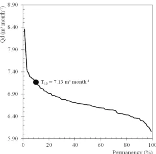
Regarding the water demand, an empiric probabilistic study was performed to determine the threshold that is expected, on average, to be equaled or exceeded in the established payback period. Figure 2 shows the water demand’s empiric flow-duration curve required by the eucalyptus seedlings. For a T of 10 years of water surplus, a demanded flow rate equal to 7.13 m3 month-1 was obtained,
Figure 2. Empiric flow-duration curve for the demanded flow rate.
According to Tatagiba et al. (2015), 70% of the maximum water retention capacity of the eucalyptus seedlings’ substrate is the threshold in which the growth and quality of the seedlings are not affected. These authors obtained a maximum evapotranspiration equal to 4.66 mm. The water depth to be applied is equal to 3.26 mm, considering 70% of the substrate water retention. Therefore, the values used for the eucalyptus seedlings evapotranspiration demand agree with the literature and ensure adequate water availability to obtain high quality pattern seedlings.
Using the model of the greenhouse coverage flow-duration curve (Equation 14), the demand for T equal to 10 years of water surplus by the crop also assumes a T of 10 years of water deficit for the reservoir. This was used to obtain the volume to be stored to supply the eucalyptus seedlings.
The reservoir’s obtained volume (the crosshatched area of Figure 1) was equal to 13.60 m3. Therefore, for the referred payback period, it is
able to store a sufficient volume to supply the water demand required by the eucalyptus seedlings in the greenhouse because the demanded water volume was 9.62 m3. Carvajal et al. (2014) studied the water
balance in RRWHs for the irrigation of an intensive agricultural system under greenhouse. The authors concluded that for the zone in the present study, it is possible to reduce the need for an external water supply in 53.02%, leading to considerable annual savings and enabling an investment in the irrigation system to improve its efficiency.
Finally, we emphasize that for a T of 10 years for the crop water surplus and a T of 10 years for the reservoir’s water deficit, the average probability of
these events to occur simultaneously is equal to 0.01%; in other words, this dimensioning is for a T of 100 years, which leads to a high safety and a lower implantation cost compared to the dimensioning performed for the same T and considering the approaches individually.
Conclusion
The new proposed RRWH dimensioning model considers the probabilistic aspects of offer (rainfall over the greenhouse coverage) and demand (evapotranspiration), thereby representing an improved method compared to the methodologies common in Brazil.
Using a probabilistic focus, it was possible to scale out an RRWH with a safety of demand supply for a payback period of 100 years, assigning a high safety and a lower cost to implant the reservoir compared with the dimensioning performed for the same payback period and considering each approach individually.
References
Associação Brasileira de Normas Técnicas [ABNT]. (2007). NBR 15527: água de chuva, aproveitamento de coberturas em áreas urbanas para fins não potáveis: requisitos. São Paulo, SP: ABNT.
Abramowitz, M., & Stegun, I. A. (1964). Handbook of mathematical functions: with formulas, graphs, and mathematical tables. North Chelmsford, US: Courier Corporation.
Akter, A., & Ahmed, S. (2015). Potentiality of rainwater harvesting for an urban community in Bangladesh. Journal of Hydrology, 528(1), 84-93.
Allen, R. G., Pereira, L. S., Raes, D., & Smith, M. (1998). Crop evapotranspiration-Guidelines for computing crop water requirements-FAO Irrigation and drainage paper 56. Rome, IT: FAO.
Amorim, S. V., & Pereira, D. J. A. (2008). Estudo comparativo dos métodos de dimensionamento para reservatórios utilizados em aproveitamento de água pluvial. Ambiente Construído, 8(2), 53-66.
Agência Nacional de Águas [ANA]. (2014). Conjuntura dos recursos hídricos no Brasil: informe 2014 encarte especial sobre a crise hídrica. Brasília, DF: ANA.
Anderson, T. W., & Darling, D. A. (1954). A test of goodness of fit. Journal of the American Statistical Association, 49(268), 765-769.
Angelocci, L. R., Sentelhas, P. C., & Pereira, A. R. (2002). Agrometeorologia fundamentos e aplicações práticas. Guaíba, RS: Agropecuária.
Carvajal, F., Agüera, F., & Sánchez-Hermosilla, J. (2014). Water balance in artificial on-farm agricultural water reservoirs for the irrigation of intensive greenhouse crops. Agricultural Water Management, 131(1), 146-155. Fernandes, L. F. S., Terêncio, D. P., & Pacheco, F. A.
(2015). Rainwater harvesting systems for low demanding applications. Science of The Total Environment, 529(1), 91-100.
Frizzone, J. A., Freitas, P. D., Rezende, R., & Faria, M. D. (2012). Microirrigação: gotejamento e microaspersão. Maringá, PR: Eduem.
Haan, C. T. (1977). Statistical methods in hydrology(2nd ed.) Ames, IA: University, Press/Ames.
Hamed, K., & Rao, A. R. (1999). Flood frequency analysis. Boca Raton, US: CRC press.
Hargreaves, G. H. (1994). Defining and using reference evapotranspiration. Journal of Irrigation and Drainage Engineering, 120(6), 1132-1139.
Horwitz, A. (2001). A version of Simpson's rule for multiple integrals. Journal of Computational and Applied Mathematics, 134(1), 1-11.
Hosking, J. R. M., & Wallis, J. R. (1997). Regional Frequency Analysis – An Approach Based on L-Moments. Cambridge, UK: Cambridge University Press.
Keller, J., & Bliesner, R. D. (1990). Sprinkle and trickle irrigation. New York, US: Van Nostrand Reinhold. Li, X. Y., Xie, Z. K., & Yan, X. K. (2004). Runoff
characteristics of artificial catchment materials for rainwater harvesting in the semiarid regions of China. Agricultural Water Management, 65(3), 211-224.
Lopes, A. D. G., Silva Junior, D. P. D., & Miranda, D. A. D. (2015). Análise crítica de métodos para dimensionamento de reservatórios de água pluvial: estudo comparativo dos municípios de Belo Horizonte (MG), Recife (PE) e Rio Branco (AC). Revista Petra, 1(2), 219-238.
Morales-Pinzón, T., Rieradevall, J., Gasol, C. M., & Gabarrell, X. (2015). Modelling for economic cost and
environmental analysis of rainwater harvesting systems. Journal of Cleaner Production, 87(1), 613-626. Naghettini, M., & Pinto, E. D. A. (2007). Hidrologia
estatística. Belo Horizonte, MG: CPRM.
Öztekin, T. (2007). Wakeby distribution for representing annual extreme and partial duration rainfall series. Meteorological Applications, 14(4), 381-387.
Rubel, F., & Kottek, M. (2010). Observed and projected climate shifts 1901–2100 depicted by world maps of the Köppen-Geiger climate classification. Meteorologische Zeitschrift, 19(2), 135-141.
Shao, Q., Zhang, L., Chen, Y. D., & Singh, V. P. (2009). A new method for modelling flow duration curves and predicting streamflow regimes under altered land-use conditions. Hydrological Sciences Journal, 54(3), 606-622. Tatagiba, S. D., Xavier, T. M. T., Torres, H., Pezzopane, J. E. M., Cecílio, R. A., & Zanetti, S. S. (2015). Determinação da máxima capacidade de retenção de água no substrato para produção de mudas de eucalipto em viveiro. Revista Floresta, 45(4), 745-754. Unami, K., Mohawesh, O., Sharifi, E., Takeuchi, J., &
Fujihara, M. (2015). Stochastic modelling and control of rainwater harvesting systems for irrigation during dry spells. Journal of Cleaner Production, 88(1), 185-195. UN-Water. (2014). UN-Water Thematic Factsheets.
Retrieved on February 23, 2014 from http://www. unwater.org/statistics/thematic-factsheets/en/
Young, S. G., Chung, E. S., Kang, W. G., & Sung, J. H. (2012). Probabilistic estimation of the storage capacity of a rainwater harvesting system considering climate change. Resources, Conservation and Recycling, 65(1), 136-144.
Received on February 19, 2016. Accepted on May 2, 2016