Observing the Existence of Low-Frequency Variability in Monthly Rainfall Data at Southeastern Brazil using R Package Tools - Neural Networks and Wavelet

1_{Institute of Aeronautics and Space (IAE), Division of Atmospheric Sciences. Praça Marechal-do-Ar Eduardo Gomes, 50. CEP: 12228-903. São José}

dos Campos. São Paulo. Brazil. E-mail: [email protected]

2_{Instituto Nacional de Pesquisas Espaciais (INPE), Computing and Applied Mathematics Laboratory, Av. dos Astronautas, 1758 - Jardim da Granja,}

OBSERVING THE EXISTENCE OF LOW-FREQUENCY VARIABILITY IN

MONTHLY RAINFALL DATA AT SOUTHEASTERN BRAZIL USING R PACKAGE

TOOLS - NEURAL NETWORKS AND WAVELET

Cleber Souza Correa¹, Haroldo Campos Velho²

ABSTRACT. This study aimed to analyze 70 years historical series in the Brazilian Southeastern region, using

monthly rainfall data. Statistical modeling techniques such as cross-wavelet spectra and artificial neural networks (ANN), from the R statistical package, were used to perform the analyses. Two different types of neural networks were employed: the multi-layer perceptron (MLP) and extreme learning machine (ELM). From the cited time series, the analysis shows the existence of a decadal and multi-decadal signal with cycles of 5, 11, and 22 years in the monthly rainfall in Brazilian Southeastern region, observing the existence of low-frequency variability. This shows a significant degree of modulation and association for the precipitation with solar activity. The neural networks were also used as forecasting tools, with a better performance for MLP-NN – smaller root mean square error. However, the MLP-NN presented a greater confidence interval than ELM-NN.

Keywords: monthly rainfall, sunspots, multi-decadal cycles

RESUMO. Este estudo teve como objetivo analisar séries históricas de 70 anos no sudeste do Brasil, utilizando

dados mensais de precipitação. Técnicas de análise estatística usando o pacote estatístico R, como espectros de wavelet cruzado e modelagem de redes neurais artificiais (RNA), foram usadas para realizar as análises. Duas implementações de redes neurais foram empregadas: multi-layer perceptron (MLP) e extreme learning

machine (ELM). Os resultados obtidos nas análises realizadas permitem inferir que as séries temporais

observadas mostram a existência de um sinal decenal e multi-decenal com ciclos de 5, 11 e 22 anos na precipitação mensal no sudeste do Brasil, observando a existência de variabilidade de baixa frequência nos dados analisados. Isso mostra um grau significativo de modulação e associação da precipitação com a atividade solar. A análise de séries temporais longas permitem a observação de variabilidades de baixa frequência, evidenciando sua grande importância e relevância. Uma significativa parcela da variância total de ciclos atmosféricos decenais é modulado pela atividade solar. As redes neurais também foram usadas como ferramentas de previsão, com melhor desempenho para a rede MLP – como mostrado pelo erro médio quadrático. A rede MLP apresentou maior amplitude no intervalor de confiança do que a rede ELM.

Palavras-chave: precipitação mensal; manchas solares; ciclos multi-decenais DOI: 10.22564/rbgf.v38i2.2046

Brazilian Journal of Geophysics (2020) 38(1): 5-19 Brazilian Journal of Geophysics

(2020) X(X): X-X

© 2020 Sociedade Brasileira de Geofísica ISSN 0102-261X

INTRODUCTION

The Sun is the major factor to establish all the dynamics of the atmosphere (Lundin et al., 2007; Love et al., 2011 and Wang et al., 2018). The inclination of the Earth's axis causes differential solar radiation incidence on the surface, producing different climatic seasons on the South and North hemispheres. Upper atmosphere dynamical systems directly respond to the forcing associated with the solar wind. Turbulent transport processes with different temporal and spatial scales are also induced for this dynamical forcing. Looking at the dynamics of this high atmosphere induces semi-stationary dynamic

processes that can influence the high

stratosphere and the tropical troposphere. The Earth-Sun system can be theorized as time-space multi-scale model, in which the Earth is directly affected by the Sun. The Earth system has a certain memory from the Sun processes,

and that end up synchronizing large

meteorological systems of the Earth with the solar activity.

In this context the dynamic processes lead to acting for the general circulation of the atmosphere, Hadley and Walker circulations, working in middle latitudes of 15 degrees of latitude in both hemispheres order. Planet Earth has large surface areas covered by oceans, which directly absorb solar radiation. The interaction of oceanic flows and atmospheric dynamics associated with processes resulting from solar activity creates a complex dynamic structure with different temporal and spatial

structures in the Earth's atmospheric and oceanic dynamics, determines and modulates the climate on our planet. Lassen and Friis-Christensen (1995) showed that the duration of the solar cycle in the last five centuries was associated with the Earth's climate, with a well-defined activity with an eleven-year cycle in the sunspots number. Indeed, the cycle has approximately 11 years, ranging from 8 to 17 years within 80 years.

Cliver (2015) discusses the cycles of solar activity and the 22-year magnetic cycle in the Sun. During the magnetic cycle, the Sun has two characteristic migrations in the behavior of sunspots, the movement towards the solar equator, and toward the poles. The motion of spots towards the equator is defined as aspects associated with Schwabe's 11-year cycles (Schwabe, 1843; Wilson, 1998) and the second is associated with the 22-year magnetic cycles, otherwise known as Hale's solar cycle (22 years) (Hale & Nicholsen, 1925; Babcock, 1961; Echer et al., 2003).

In Corrêa et al. (2019), using wavelet and cross-wavelet analysis, multidecadal cycles were observed between the monthly number of spots and the South Oscillation (IOS) and Pacific Decadal Oscillation (DOP) indexes. Showing cycles of 2.66, 5.33, 10.66, and 21.33 years. It was also compared to the average monthly rainfall in the meteorological stations of the airports of Belém, Fortaleza, São Luiz, and Natal, showing that in the north/northeast of Brazil the multidecadal cycles of precipitation accompanied the variability of the sunspots, with an intense signal of 11 years and less intense of 22 years.

Corrêa et al. (2020) using the 1951-2017 historical series of the Atlantic Meridional Mode (AMM) index and the monthly number of sunspots, it was possible to observe a high correlation between them. The use of wavelet and cross-wavelet analysis showed the presence of multidecadal cycles pronounced in eleven years, as well as cycles of 2.66 and 5.33. AMM index showed, in the part of the Sea Surface Temperature (SST), the presence of a weak signal of 21.33 years. Influence and association of sunspot variability on surface temperature in the Northern and Northeastern regions of Brazil. The time series of monthly rainfall shows a very complex behavior, but the methodology using Cross-wavelet allowed us to observe the correlation in the Brazilian tropical region between the long historical series of monthly rainfall and the sunspot series. Allowing associated multidecadal cycles with rainfall observed. An environmental variable such as rainfall has a behavior that can be dismembered at different spatial scales such as mesoscale or macro scale, as well as at a regional synoptic level. As its statistical properties behave Rainfall stochastic, temporal variability and spatially organizes itself at the mesoscale level in clusters or random or fractal behavior. Kim et al. (2013) show that the stochastic rainfall generators are classified into the three following categories: (1) the multi-scaling models, which are based on the observation that rainfall patterns have ‘‘self-similarity’’ at a given range of timescales, (2) the nonparametric resampling models, which forms the new rainfall time series by borrowing the

fragments from the instrumental data with similar statistical properties, (3) the Poisson cluster rainfall models, which is being considered in this study. The Poisson cluster rainfall models (Rodriguez-Iturbe et al., 1987, 1988), a type of stochastic rainfall models, represent rainfall as a sequence of storms composed of rain cell clusters (Kavvas & Delleur, 1975).

As for frequency and spatial variability, Mazzarella (1999) shows that an appreciation of the fractal dimension dependence and the specific scaling region on intensity threshold is the key to understanding that the rainfall is a

multifractal process in which its spatial

distribution is organized into clusters of high rainfall localized cells embedded within clusters of lower intensity small mesoscale areas. These areas are within clusters of still lower intensity large mesoscale areas, which are contained within some synoptic-scale lowest intensity rainfall fields.

Brunsell (2010) shows that since the physical processes encompassing rainfall range

from micro-scales (e.g. turbulence, cloud

formation processes) to interannual climatic variability (e.g. Pacific Decadal Oscillation, El Niño Southern Oscillation, the Atlantic Ocean

multidecadal and interdecadal processes),

characterizing the scaling properties of rainfall is essential for understanding precipitation. This has led researchers to adopt many of the techniques used in chaos theory and non-linear dynamics (Dhanya & Nagesh Kumar, 2010; Jothiprakash & Fathima, 2013; Yildirim & Altinsoy, 2017) and multifractals (Breslin &

Belward, 1999; Veneziano et al., 2006; Maskey et al., 2019).

Currently, longer historical series are

available of meteorological parameters and in this case, we are interested to analyze the southeastern Brazilian Rainfall. As Brazil is a continental country what would be the behavior of rainfall in southeastern Brazil. It would accompany solar activities about the number of sunspots such as the work of Corrêa et al. (2019) to the north and northeast of Brazil. A time series of total monthly precipitation may present extreme values and irregularities associated with the structure composed of different spatial and temporal scales that make up the total monthly observed value. Thus, we seek to use a framework of tools such as Wavelet analysis and neural networks to analyze historical series and to evaluate the ability to make predictions with different neural network models, with complex

historical rainfall series, as well as their association and influence of solar activity with the historical series of sunspots.

METHODOLOGY

The computational tools for data analysis are presented in this section.

Wavelet analysis

The WaveletComp versions 1.0 and 1.1 is routine from the R-package for data analysis based on univariate and bivariate time series wavelets (Roesch & Schmidbauer, 2014, 2016). The

WaveletComp applies with the frequency

analysis of uni- and bivariate time series using Morlet wavelet (Morlet et al., 1982a, 1982b; Goupillaud et al., 1984), and the biwavelet package (Grinsted et al., 2004). Morlet wavelet is the version implemented in WaveletComp. The

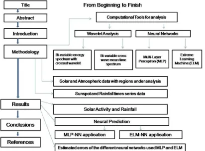
Figure 1. The graphical diagram that explains the methodology used

cross-wavelet function allows filtering different frequency between two time series, allowing the passage of frequency signals that are similar in both time series. The Morlet wavelet transform of a time series (xt) is defined as the convolution of the series with a set of "wavelet daughters" generated by the "mother wavelet" by time translation by  and defining the scale by s. Morlet wavelet, in the WaveletComp routine, is expressed as:

y

(t) =

p

e

e

The "angular frequency" ω (or rate of rotation in radians per unit time) is defined as ω = 6, which is the preferred value in the literature

since the Morlet wavelet is solved

approximately in an analytical way; and with an oscillation equals 2π (radians); therefore,

the period (or the inverse frequency)

measured in units of time is equal to 2π/6. The Morlet wavelet transform of a time series (xt) is computed by "wavelet daughters" generated from the "mother wavelet" by time translation  and the scale s – see equation below:

wave(

t

, s) =

x

1

s

å

y

t

-

t

s

æ

è

ç

ö

ø

÷

The position of the daughter wavelet in the time domain is determined by the location of the time

parameter  being displaced by t a time

increment. The square of the amplitude has an

interpretation as time-frequency (or time-period) wavelet energy density, and is called the wavelet power spectrum (Carmona et al.,1998):

Power(

t

, s) =

1

s

wave(

t

, s)

2 ₍₃₎

In the case of white noise, its expectation at each time and scale corresponds to the series variance (with proportionality factor 1/s in this

rectified version of wavelet power).

WaveletComp rectifies the wavelet power spectrum (cross-wavelet) according to Veleda et al. (2012).

Smoothing for the time period and/or direction is necessary to perform the calculation with the Coherence wavelets methodology with their multiples (Liu, 1994). The set choice of scales s determines the series wavelet coverage in the frequency domain. The rainfall/sunspot data was

read by software R using the library

(WaveletComp) with files in the format comma-separated values (csv).

Neural Networks

The NNFOR routine from version 0.9.6 (2019) in

R-package was employed to generate

forecasting time series operators by neural networks (NN), following Crone & Kourentzes (2010) and Kourentzes et al. (2014). The NNFOR package has an implementation for Multi-layer

Perceptron (MLP) and Extreme Learning

Machine (ELM). The package NN default parameters were applied. It is important to remember that the usual purpose to train the

multilayer perceptron is to get good generalization in unseen data, for example in time series forecasting applications.

Maximum generalization performance will occur before the general training network error reaches a minimum value. A network is considered to be trained when a minimum difference between the network output and a reference set is reached. However, a cluttered data set can result in a network's worst predictive ability. One way to avoid such fail, for producing a good generalization performance, is to split the training data into multiple sets: – a training set, a validation set, and a test set. The training set is used to compute weight connection for the network. The validation set can be used to assess the generalizability of the network, while training is taking place. Training is interrupted when generalization performance is reached. This technique is known as early stopping and is particularly useful when training multilayer Perceptrons with real and noisy data. Finally, the test suite is used to evaluate the overall

performance of the trained network

(Schmidhuber, 2015). In this respect, three data networking training sessions were analyzed. The first one considering the full series, from January 1951 to June 2018. The second is taken from January 1951 to June 1990. Finally, the third period is from January 1990 to June 2010, all with a 36-month forecast window.

The accuracy function of the R package Forecast was used to estimate the errors in the rainfall series forecasting estimates with the three

trained neural networks, the proposed

methodology was used by Hyndman & Koehler (2006) and Hyndman & Athanasopoulos (2014). The measures calculated are: Root Mean Squared Error (RMSE) Eq. (4) is a quadratic scoring rule which measures the average magnitude of the error. The square difference between forecast and corresponding observed values is calculated and then averaged over the sample. Since we are dealing with square difference, the RMSE gives a relatively high weight to large errors. The Mean Absolute Error (MAE) Eq. (5) is a linear score, which means that all individual differences are weighted equally on the average, measuring the average magnitude of errors in a set of forecasts, and it is used to measure accuracy for continuous variables. Where 𝑦̂ are the predicted values, 𝑦𝑖 𝑖 are the

observed values and n the number of observations. The equations for RMSE and MAE are shown below:

(4)

(5)

Multi-layer Perceptron (MLP)

There is an R-routine to configure an MLP neural network for time series forecasting. MLP architecture can be seen as a general practical

Specifically, let k be the number of network inputs and m the number of outputs. The network input-output relationship defines a mapping from a k k-dimensional input Euclidean space to an output m-dimensional Euclidean space, which is infinitely continuously differentiable (Gardner & Dorling, 1998).

The most commonly used form of Neural Networks for forecasting is the feedforward

Multilayer Perceptron. The one-step-ahead

forecast 𝑌̂𝑛+1 _{is computed using inputs that are}

lagged observations of the time series or other explanatory variables. I denote the number of inputs Pi of the Neural Network. Their functional

form is:





_

_

where w = (β,y) are the network weights with β =

[β1, . . . , βH], y = [y11, . . . , yHK] for the output and the hidden layers respectively. Pk this term refers

to the neuron’s inputs. The β0 and y0n are the

biases of each neuron, which for each neuron act similarly to the intercept in a regression, H is the number of hidden nodes in the network, and g(·) is a non-linear transfer function, which the default is using hyperbolic tangent, Kourentzes et al. (2014).

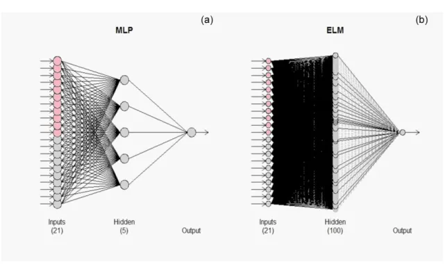
Figure 2a shows the MLP neural network structure used with 21 inputs, one hidden layer with 5 neurons. The package applied a procedure to determine the number of inputs to

feed the NN: the process included to add more and more previous precipitation values, recorded from different times, to predict the future precipitation.

Extreme Learning Machine (ELM)

ELM is a learning algorithm for single hidden layer feedforward neural networks, is very efficient and effective, such development is described in the work of Huang et al. (2006) and Ord et al. (2017). To minimize the network cost function, ELM theories claim that the hidden nodes’ learning parameters can be assigned randomly without considering the input data. Then, becomes a linear system, and the output of its weights can be analytically determined by finding the least-squares solution, in which we will have an inverse matrix being the generalized inverse of a Moore-Penrose matrix. So, calculation of the output weights is done by a mathematical transformation, which avoids any lengthy training phase where the parameters of the network are adjusted iteratively with some appropriate learning parameters (such as learning rate and iterations). The historical rainfall data series were read by software R using the library (Forecast and NNFOR routine) with files in the format comma-separated values files (csv), as well as programs were written and saved in individual files for each observation location. Figure 2b shows the ELM neural network with 21 inputs, one hidden layer with 100 hiddens neurons – the same mentioned strategy to select the number of input values is also adopted here.

Solar and atmospheric data, with regions under analysis

Numerous scientific articles are associating solar activity with atmospheric and oceanic dynamic systems (Tobias & Weiss, 2000; Kodera & Kuroda, 2002; Coughlin &Tung, 2004; Meehl et al., 2009; Roy & Haigh, 2010; Mazzarella et al., 2010; Abalos et al., 2014; Linz et al., 2019).

In the work of Kodera & Kuroda (2002) showed that the dynamic impact of the 11-year solar cycle is associated in the stratopause region, where ultraviolet solar heating is greatest. The most important variation in solar forcing is longer than the day cycle is the annual cycle. Thus, the climatic characteristics of the zonal wind variation associated with the annual cycle were initially studied to characterize the basic characteristics of the dynamic response of the atmosphere to changes in solar radiative forcing,

which is important to characterize low-frequency cycles in multidecadal processes. The results of the analysis suggest that in an average

climatological state, stratopause circulation

evolves from a radiation controlled state to a dynamically controlled state during winter in both

hemispheres. The transition period is

characterized by a change to the west side of the jet streams at altitude. The effect of the solar cycle appears as a change in the balance between radiatively and dynamically controlled states. The radiation-controlled state lasts longer during the solar maximum phase, and the stratopause subtropical jet reaches a higher velocity. The great dynamic response to relatively weak radiative forcing can be understood by the bimodal nature of the winter atmosphere due to the interaction with the southern propagating planetary waves and the zonal mean winds. It is

Figure 2.Two neural network models used in this work (a) Multi-layer Perceptron, and (b) Extreme

suggested that the solar influence produced in the upper stratosphere and stratopause region be transmitted to the lower stratosphere by (1) modulating the internal mode of variation in the night polar jet, this process is significant in the mid and high latitudes and (2) a change in Brewer-Dobson circulation (Abalos et al., 2014; Linz et al., 2019) is prominent in the equatorial region.

However, the influence of solar activity is very large not only on the surface but on stratospheric

levels and the high stratosphere and

thermosphere. In which the atmosphere is influenced by the interaction of the solar wind in the tropical region. The equatorial-stratospheric wind oscillates between easterly and westerly directions and with a period around 22 to 32 months called Quasi Biennal Oscillation (QBO). In the work of Mazzarella et al. (2011) showed that QBO may have the dominant period of 28 months has been reaffirmed but with a discernible amplitude and a phase, respectively, inversely varying with height. Such a cycle suggests an estimate for the coming easterly equatorial wind occurrence at 15 hPa level at the end of 2009. The 28-month harmonic is found to take about a year to descend from 15 to 70 hPa with a progressive lag of about 1 month/km. At the top of the stratosphere, easterlies dominate, while at the bottom, westerlies are more likely to be found. Correlation with sunspot numbers and seasonal rainfall was discussed.

Roy & Haigh (2010) identified signs of the solar cycle in 155 years of global sea level pressure (SLP) and sea surface temperature

(SST) using a multiple linear regression approach. Found in the North Pacific a statistically significant difference the weakening of Aleutian's low-pressure system and a shift to the north of the Hawaiian’s high-pressure system in response to higher solar activity, confirming the results of previous authors using different techniques. They also find a weak but wide reduction in pressure on the equatorial Pacific. In the SST, they identified a weak El Niño as a standard in the tropics for the 155 years. It showed that the last years analyzed were influenced by the data composition technique of the sunspot peak years cycle because these years have often coincided with the negative phase of the El Niño-Southern Oscillation (ENSO) cycle.

Solar activity acts on the earth system by modulating various physical scales and different time scales involved. Therefore the monitoring of meteorological variables with the monthly rainfall may show a certain degree of association with solar cycles, in a low-frequency analysis.

The monthly time series analyzed were obtained from the Sunspot of the World Data Center SILSO, Royal Observatory of Belgium,

Brussels (see the link:

http://www.sidc.be/silso/datafiles), which was

transferred the data file (SN_m_tot_V2.csv) with information, years from 1951 up to 2018 with 68 annual series. Monthly rainfall data were obtained from the Aeronautics Command of the Airspace Control Department (DECEA, Brazil) Climatological Database, the DECEA climate

database is available in the link:

http://clima.icea.gov.br/clima/. Monthly rainfall

data were from the following locations:

Congonhas airport, Guarulhos airport, and Campinas airport, São Paulo state, Brazil. In the Rio de Janeiro state – Brazil, the Santa Cruz

airbase and Santos Dumont airport were considered. The time series used followed the sunspot period from January 1951 up to June 2018. Monthly precipitation data in the historical series showed very complex characteristics, with huge spatial variety, and non-stationary or semi-stationary behavior.

RESULTS

Solar Activity and Rainfall

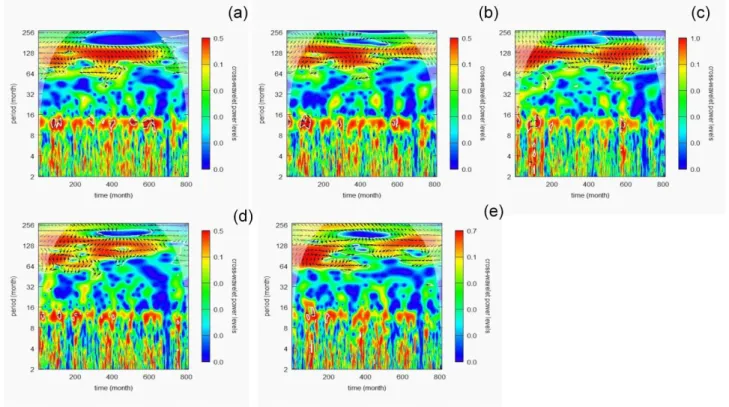
Figure 3 shows the cross-wavelet spectrum that in all figures a significant 11-year signal associated with the solar cycle. It also has cycled in 32 and 60 months, cycles of 3 and 5 years. Solar activity within the solar time series has a peak between the 1960s and 1970s and the end Figure 3. The bi-variable energy spectrum with crossed wavelet being Monthly Rainfall and Sunspot, (a) Congonhas Airport, (b) Guarulhos Airport, (c) Campinas Airport, (d) Santa Cruz Airbase, and (e) Santos Dumont Airport.

of the 2010- 2020 time series is a solar minimum. The cross-wavelet spectra show a decrease at the end of the series following the solar minimum, in the figures (a) Congonhas airport and (d) Santa Cruz airbase.

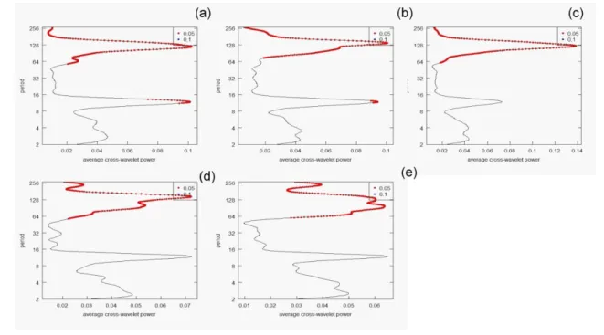
Figure 4 shows the mean bi-variable cross-wave time spectrum between monthly rainfall and sunspots, showing significant signs at 11 years, with cycles at 60 months. In the figures (d) Santa Cruz airbase and (e) Santos Dumont shows a weak signal in 22 years but significant.

Observed monthly rainfall data in

southeastern Brazil show that rainfall follows 11-year multidecadal solar cycles and can also follow 5-year and/or 22-year cycles, which are observed in the mean bi-variable cross-wave time spectrum (Fig. 3). The work by Kodera & Kuroda (2002) shows that the dynamic impact of the 11-year solar cycle is associated in the

stratopause region, where ultraviolet solar heating is greatest. The most important variation in solar forcing is the annual cycle. Thus, the climatic characteristics of the zonal wind variation associated with the annual cycle are observed as basic characteristics of the atmospheric dynamic response to solar radiative forcing changes, which is important to characterize low-frequency cycles in multidecadal processes, as observed in the wavelet analysis. Which can be interpreted in

the monthly rainfall series analyses in

southeastern Brazil. The results suggest that the radiation-controlled state lasts longer during the maximum solar phase, and the stratopause subtropical jet reaches a higher velocity. This would directly affect the meteorological dynamics in the southern hemisphere and its effects felt in South America. More specifically in southeastern Brazil. Figure 3 also appears a 12-month signal

Figure 4.The bi-variable cross-wave mean time spectrum being Monthly Rainfall and Sunspot, (a)

Congonhas Airport, (b) Guarulhos Airport, (c) Campinas Airport, (d) Santa Cruz Airbase, and (e) Santos Dumont Airport.

in all monthly rainfall series.

Neural Prediction MLP-NN application

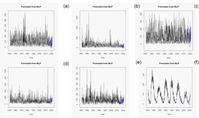
The historical series of monthly total rainfall shows great variability among the analyzed series although these are from a relatively close region located in southeastern Brazil. The maximum total values of the monthly rainfall present different intensities, in each analyzed series, result in the complexity involved in the different possible meteorological mechanisms and spatial differences that cause the maximum values of rainfall. Figures 5 and 6 show the maximum monthly rainfall at (b) Guarulhos airport of 1773.4 millimeters (mm) in February

1963 and (e) Santos Dumont airport of 688 mm in November 1959. The neural networks have difficulty predicting these extreme values in the monthly rainfall series, with low recurrence. However, these peaks occur in the early 1960s and also follow the maximum value of the 70-year sunspot series, which occurred from 1957 to 1960, the highest absolute recent solar activity in the sunspot series, in this period. Solar activity has fallen to lower peaks until June 2018. Other monthly rainfall peaks also occurred with solar activity peaks. Such a situation shows a definite significant degree of association between solar activity and atmospheric processes. This could be used as a predictor of extreme monthly rainfall values in southeastern Brazil. However, the use of the neural network implies an input that was

Figure 5. Total series of monthly rainfall (1951-2018) with respective forecasts of 36 months at the end of the

observed series, the forecast is in blue, using the MLP neural network model: (a) Congonhas Airport, (b) Guarulhos Airport, (c) Campinas Airport, (d) Santa Cruz Airbase, and (e) Santos Dumont Airport and (f) Sunspot

used in this work in the time series of the order of 21 elements to train the network, as these may not use the extreme values of the neural network may have limitations in predicting these extremes value. As the neural networks were trained in a period in which it can be understood by minimal solar activity, the behavior of the network was adequate because the monthly rainfall had variability close to an average behavior.

Figures 5 and 6 with the total series of Monthly rainfall can be seen that the historical series analyzed bring in their observations a set of characteristics that may indicate local physical characteristics and may also in certain values in

some respect be compounded, spatially

associated with the transport performed because the rainfall is within processes that may have a

broader scope. Therefore the total result of rainfall is a value composed of local and also propagation processes. It can be understood by

creating non-stationary or semi-stationary

patterns. This behavior can characterize a type of memory of these processes that are recorded in the temporal series and can give a picture of the physical processes observed in the maximum or minimum of the analyzed data.

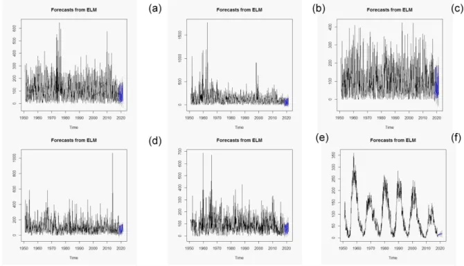
Figure 6. Total series of monthly rainfall (1951-2018) with respective forecasts of 36 months at the end of the

observed series, the forecast is in blue, using the ELM neural network model: (a) Congonhas Airport, (b) Guarulhos Airport, (c) Campinas Airport, (d) Santa Cruz Airbase, and (e) Santos Dumont Airport and (f) Sunspot

For this reason, it shows great complexity, because although the localities are relatively close, the observed values may present distinct values in the intensity for certain simultaneous months in the temporal series. In this respect, the graphs showed a consistent predictive behavior by the estimates made by the two neural network models used, MLP and ELM. Table 1 presents the values of errors estimated by the use of different methodologies in neural networks. For short series analysis, the MLP network model presented better results with smaller errors. ELM-NN application

The ELM network model was sensitive to how long the time series is. Shorter time series present worse results in comparison to the longer

time series. Therefore, a longer time series improve the adjustments, implying in a smaller error with the longer analyzed time series.

For this reason, it shows great complexity, because although the localities are relatively close, the observed values may present distinct values in the intensity for certain simultaneous months in the temporal series. In this respect, the graphs showed a consistent predictive behavior by the estimates made by the two neural network models used, MLP and ELM. The computed prediction by neural networks is performed by the R-routine called “forecast”, where the forecasting value and the confidence interval are calculated.

Figures 7 and 8 show the analysis of the shorter series from 1951 to 1990, using the different neural network architectures the MLP neural network model did not show to be

Figure 7. Total series of monthly rainfall (1951-1990) with respective forecasts of 36 months at the end of the

observed series, the forecast is in blue, using the MLP neural network model: (a) Congonhas Airport, (b) Guarulhos Airport, (c) Campinas Airport, (d) Santa Cruz Airbase, and (e) Santos Dumont Airport.

Figure 8. Total series of monthly rainfall (1951-1990) with respective forecasts of 36 months at the end of the

observed series, the forecast is in blue, using the ELM neural network model: (a) Congonhas Airport, (b) Guarulhos Airport, (c) Campinas Airport, (d) Santa Cruz Airbase, and (e) Santos Dumont Airport.

sensitive to the time series size, the weak gray lines show the confidence interval associated to the forecast value (blue line), hereafter this will be the adopted colour convenction in the present study. The MLP model has greater deviations from the forecast variance in relation to the ELM. Figures 9 and 10 somewhat followed the results observed in the 70-year-old neural network analysis, the MLP and ELM neural network models were similar to the total series analysis.

The results presented by the two different neural networks, had good results even using simpler models, Figure 11 (a) at Congonhas airport, showed good results with a relatively simple MLP and ELM model. The models of more complex neural networks can be tested obtaining more adequate results with greater computational processing. The worst result could

be observed at Guarulhos airport (Fig. 11 (b)) because the RNN models were not able to represent the maximums, as the temporal series of this location showed greater non-linearities, as it has the highest values of monthly rainfall.

Table 1 presents the values of errors estimated by the use of different methodologies in neural networks. For short series analysis, the MLP network model presented better results with smaller errors. However, the ELM network model showed that it was sensitive to the increase of the time series improving the adjustments and having a smaller error with the increase of the analyzed time series.

Table 1 showed a better result with less error in the MLP neural network estimates in concerning ELM, in all analyzes performed.

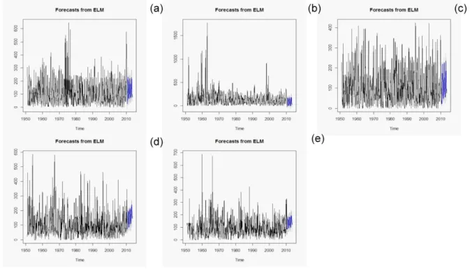
Figure 9. Total series of monthly rainfall (1951-2010) with respective forecasts of 36 months at the end of the

observed series, the forecast is in blue, using the ELM neural network model: (a) Congonhas Airport, (b) Guarulhos Airport, (c) Campinas Airport, (d) Santa Cruz Airbase, and (e) Santos Dumont Airport.

CONCLUSIONS

The results obtained from the time-series analyzes show the existence of a decadal and multi-decadal signal with cycles of 5, 11, and 22 years in the monthly rainfall for the Southeastern region in the Brazil. A low-frequency variability signal is observed. Therefore, there is a degree of association and modulation with solar activity. In other words, the precipitation signal variability has a memory synchronized with solar variability.

Neural networks were designed for emulating the rainfall behaviour, and they were also employed as a forecasting tool. The MLP-NN presented a better performance than ELM-NN. However, as mentioned in the section “ELM-NN application”, the MLP-NN obtained a greater magnitude for confidence interval than ELM-NN.

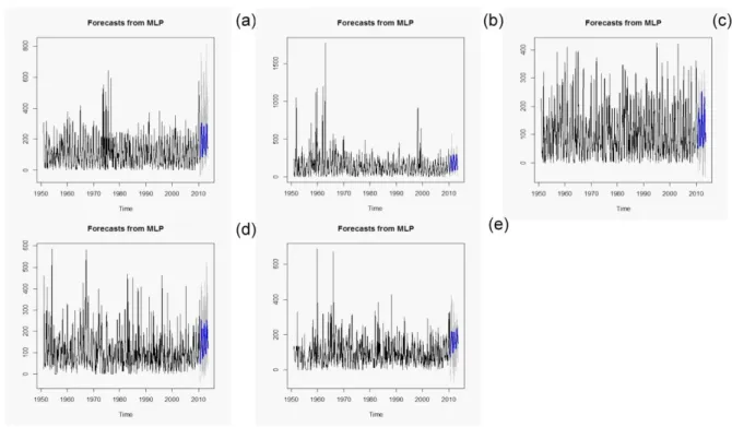
Figure 10. Total series of monthly rainfall (1951-2010) with respective forecasts of 36 months at the end of the

observed series, the forecast is in blue, using the MLP neural network model: (a) Congonhas Airport, (b) Guarulhos Airport, (c) Campinas Airport, (d) Santa Cruz Airbase, and (e) Santos Dumont Airport.

The historical maximums of monthly rainfall in the analyzed series occurred after the maximums of solar activity, showing coherence. Kodera & Kuroda (2002) showed that the association of the 11-year solar cycle dynamics is associated in the stratopause region, where ultraviolet solar heating is greater. The most important variation in solar forcing is its temporal influence is greater than the annual cycle. Thus, the climatic characteristics of the variation in the circulation model are associated with the annual cycle and are linked to the dynamic response of the atmosphere to changes in solar radiative forcing, which is important to characterize low-frequency cycles in multidecadal processes. Such complex characteristics possibly create configurations that are influenced by solar variability produce certain circulations in the upper stratosphere and region

of the stratopause, and these are transmitted and can influence the lower stratosphere. This may ratify the behavior of the atmospheric dynamics, this process being significant at medium and high latitudes and its importance in the role of the

Brewer-Dobson circulation (Gerber, 2012;

Butchart, 2014), which is prominent in the equatorial region.

Other works will be carried out to apply a similar methodology to other Brazilian regions with longer time series. Maybe, time-series with longer observation time periods will allow associating the second maximum of solar activity and the maximum values of monthly rainfall. The neural network modeling allowed us to generate useful estimates for the monthly rainfall.

Figure 11. Neural network predictions MLP model (blue line), RNN ELM model (red line) and observation of

monthly precipitation (green line) between July 2018 to May 2020, (a) Congonhas Airport, (b) Guarulhos Airport, (c) Campinas Airport, (d) Santa Cruz Airbase, and (e) Santos Dumont Airport.

REFERENCES

ABALOS M, RANDEL WJ & SERRANO E. 2014. Dynamical Forcing of Subseasonal Variability in the Tropical Brewer–Dobson Circulation. J. Atmos. Sci., 71: 3439–3453.

BABCOCK HW. 1961. The topology of the Sun’s magnetic field and the 22-year cycle. Astrophys. J. 133: 572–587.

BUTCHART, N. 2014. The Brewer-Dobson circulation. Rev. Geophys., 52: 157–184.

BRESLIN MC & BELWARD JA. 1999. Fractal dimensions for rainfall time series. Mathematics and Computers in Simulation. 48(4-6): 437-446. BRUNSELL NA. 2010. A multiscale information theory approach to assess spatial–temporal variability of daily precipitation, Journal of Hydrology, 385(1–4): 165-172.

CLIVER EW. 2015. The Extended Cycle of Solar Activity and the Sun’s 22-Year Magnetic Cycle. In: BALOGH A, HUDSON H, PETROVAY K & VON STEIGER R. (Eds.). The Solar Activity Cycle. Space Sciences Series of ISSI, 53: 169-189. Springer, New York, NY.

CARMONA R, HWANG W-L & TORRESANI B. 1998. Practical Time Frequency Analysis. Gabor and Wavelet Transforms with an Implementation in S. Academic Press, San Diego.

CORRÊA CS, GUEDES RL, CORRÊA KAB & PILAU FG. 2019. Multidecadal Cycles Study in the Climate Indexes Series Using Wavelet Analysis in North/Northeast Brazil. Anuário do Instituto de Geociências – UFRJ, 42(1): 66-73.

CORRÊA CS, GUEDES RL, DA ROCHA AMM & CORRÊA KAB. 2020. Multidecadal Cycles of the

Table 1. Estimated errors of the different neural networks used MLP and ELM by the accuracy function of the Forecast

Climatic Index Atlantic Meridional Mode: Sunspots that Affect North and Northeast of Brazil. J Aerosp Tecnol Manag, 12(e0420).

COUGHLIN K & TUNG KK. 2004. Eleven-year

solar cycle signal throughout the lower

atmosphere, J. Geophys. Res., 109: D21105. CRONE SF & KOURENTZES N. 2010. Feature selection for time series prediction – A combined filter and wrapper approach for neural networks. Neurocomputing, 73(10): 1923-1936

DHANYA CT & NAGESH KUMAR D. 2010. Nonlinear ensemble prediction of chaotic daily rainfall, Advances in Water Resources, 33(3): 327-347.

ECHER E, RIGOZO NR, NORDEMANN DJR, VIEIRA LEA, PRESTES A & DE FARIA HH. 2003. Revista Brasileira de Ensino de Física, 25(2): 157-163.

GARDNER M & DORLING SR. 1998. Artificial neural networks (the multilayer perceptron) - a review of applications in the atmospheric sciences. Atmospheric Environment, 32(14/15): 2627-2636.

GERBER EP. 2012. Stratospheric versus Tropospheric Control of the Strength and Structure of the Brewer–Dobson Circulation. J. Atmos. Sci., 69: 2857–2877.

GOUPILLAUD P, GROSSMAN A & MORLET J. 1984. Cycle-octave and related transforms in seismic signal analysis. Geoexploration, 23: 85–

102.

GRINSTED A, MOORE JC & JEVREJEVA S. 2004. Application of the cross wavelet transform and wavelet coherence to geophysical time series. Nonlinear Processes in Geophysics, 11: 561-566.

HALE GE & NICHOLSON SB. 1925. The law of sun-spot polarity. Astrophys. J., 62: 270-300. HYNDMAN RJ & ATHANASOPOULOS G. 2014. Optimally reconciling forecasts in a hierarchy. Foresight, vol. Fall 2014, 35: 42-48.

HYNDMAN RJ & KOEHLER AB. 2006. Another

look at measures of forecast accuracy.

International Journal of Forecasting, 22(4): 679-688.

HUANG GB, ZHOU H & DING X. 2006 Extreme learning machine: theory and applications. Neurocomputing, 70(1): 489-501.

JOTHIPRAKASH V & FATHIMA TA. 2013. Chaotic analysis of daily rainfall series in Koyna reservoir catchment area, India. Stochastic Environmental Research and Risk Assessment, 27: 1371.

KAVVAS ML & DELLEUR JW. 1975. The stochastic and chronologic structure of rainfall

sequences —Application to Indiana. Technical

Report 57. Water Resources Research Center, Purdue University, West Lafayette.

KIM D, OLIVERA F & CHO H. 2013. Effect of the inter-annual variability of rainfall statistics on

stochastically generated rainfall time series: part 1. Impact on peak and extreme rainfall values. Stoch Environ Res Risk Assess, 27: 1601.

KODERA K & KURODA Y. 2002. Dynamical response to the solar cycle. J. Geophys. Res., 107(D24): 4749.

KOURENTZES N, BARROW BK & CRONE SF. 2014 Neural network ensemble operators for time series forecasting. Expert Systems with Applications, 41(9): 4235-4244.

LASSEN K & FRIIS-CHRISTENSEN E. 1995. Variability of the solar cycle length during the past five centuries and the apparent association with terrestrial climate. Journal of Atmospheric and Terrestrial Physics, 57(8): 835-845.

LINZ M, ABALOS M, GLANVILLE AS,

KINNISON DE, MING A & NEU JL. 2019. The global diabatic circulation of the stratosphere as a metric for the Brewer–Dobson circulation. Atmospheric Chemistry and Physics, 19: 5069-5090.

LIU PC. 1994. Wavelet spectrum analysis and ocean wind waves. In: FOUFOULA-GEORGIOU E & KUMAR P (Eds.). Wavelets in Geophysics, Academic Press, San Diego, 151–166.

LOVE JJ, MURSULA K, TSAI VC & PERKINS

DM. 2011. Are secular correlations between sunspots, geomagnetic activity, and global temperature significant? Geophysical Research Letters, 38: L21703.

LUNDIN R, LAMMER H & RIBAS I. 2007.

Planetary Magnetic Fields and Solar Forcing: Implications for Atmospheric Evolution. Space Sci. Rev., 129: 245–278.

MASKEY ML, PUENTE CE & SIVAKUMAR B. 2019. Temporal downscaling rainfall and stream flow records through a deterministic fractal geometric approach, Journal of Hydrology, 568: 447-461.

MAZZARELLA A. 1999. Multifractal Dynamic Rainfall Processes in Italy. Theor. Appl. Climatol., 63: 73-78.

MAZZARELLA A, GIULIACCI A & LIRITZIS I. 2010. On the 60-month cycle of multivariate ENSO index. Theor. Appl. Climatol., 100: 23–27. MAZZARELLA A, GIULIACCI A & LIRITZIS I. 2011. QBO of the Equatorial-Stratospheric Winds Revisited: New methods to verify the dominance of 28-month cycle. International Journal of Ocean and Climate Systems. 2(1): 19-26.

MEEHL GA, ARBLASTER JM, MATTHES K, SASSI F & VAN LOON H. 2009. Amplifying the Pacific Climate System Response to a Small 11-Year Solar Cycle Forcing. Science, 325: 1114-1118.

MORLET J, ARENS G, FOURGEAU E & GIARD D. 1982a. Wave propagation and sampling theory – Part I: complex signal and scattering in multilayered media. Geophysics, 47: 203–221. MORLET J, ARENS G, FOURGEAU E & GIARD D. 1982b. Wave propagation and sampling

waves. Geophysics, 47: 222–236.

ORD K, FILDES R & KOURENTZES N. 2017. Principles of Business Forecasting. 2nd ed., Wessex Press Publishing Co., chapter 10.

ROESCH A & SCHMIDBAUER H. 2014. WaveletComp: Computational Wavelet Analysis. https://cran.r-project.org/package=WaveletComp. ROESCH A & SCHMIDBAUER H. 2016. WaveletComp 1.1: A guided tour through the R package.

http://www.hsstat.com/projects/WaveletComp/Wa veletComp_guided_tour.pdf.

RODRIGUEZ-ITURBE I, COX DR & ISHAM V. 1987. Some models for rainfall based on stochastic point processes. Proc R Soc Lond Ser, A410(1839): 269–288.

RODRIGUEZ-ITURBE I, COX DR & ISHAM V. 1988. A point process model for rainfall: further

developments. Proc R Soc Lond Ser,

A417(1853): 283–298.

ROY I & HAIGH JD. 2010. Solar cycle signals in sea level pressure and sea surface temperature. Atmos. Chem. Phys., 10: 3147-3153.

SCHMIDHUBER J. 2015. Deep learning in neural networks: An overview. Neural Networks, 61: 85-117.

SCHWABE M. 1843. Die Sonne. Astronomische Nachrichten, 20: 283-286.

TOBIAS SM & WEISS NO. 2000. Resonant Interactions between Solar Activity and Climate.

J. Climate, 13: 3745–3759.

VELEDA D, MONTAGNE R & ARAUJO M. 2012. Cross-Wavelet Bias Corrected by Normalizing Scales. Journal of Atmospheric and Oceanic Technology, 29: 1401–1408.

VENEZIANO D, LANGOUSIS A & FURCOLO P. 2006. Multifractality and rainfall extremes: a review. Water Resources Research, 42(6): 1-18. WANG W, MATTHES K, TIAN W, PARK W, SHANGGUAN M & DING A. 2018. Solar impacts on decadal variability of tropopause temperature and lower stratospheric (LS) water vapour: a mechanism through ocean–atmosphere coupling. Climate Dynamics, 52: 5585–5604.

WILSON RM. 1998. A Comparison of Wolf’s

Reconstructed Record of Annual Sunspot Number with Schwabe’s Observed Record of ‘Clusters of Spots’ for the Interval of 1826–1868. Solar Physics, 182: 217–230.

YILDIRIM HA & ALTINSOY HA. 2017. Chaos and trend analysis of monthly precipitation over Arabian Peninsula and Eastern Mediterranean. Arabian Journal of Geosciences, 10: 1-12.