Faculdade de Ciências
Departamento de Física
EVALUATION OF THE D-SPECT SYSTEM:
Region Centric Acquisition and Tracer Kinetics
Filipa Alexandra Pina Barrento da Costa
Dissertação
Mestrado Integrado em Engenharia Biomédica e Biofísica
Faculdade de Ciências
Departamento de Física
EVALUATION OF THE D-SPECT SYSTEM:
Region Centric Acquisition and Tracer Kinetics
Filipa Alexandra Pina Barrento da Costa
Dissertação de Mestrado Integrado Orientada pelo Professor Pedro Almeida e pelo
Professor Brian Hutton
Mestrado Integrado em Engenharia Biomédica e Biofísica
i
ACKNOWLEDGEMENTS
I would like to acknowledge all the people that made this thesis possible.
First I would like to thank my supervisor Professor Brian Hutton for the critical insights and enthusiastic support and guidance throughout the work and my supervisor in Portugal, Professor Pedro Almeida for helping me to find this opportunity of making this thesis at UCL, and for being always available. I also want to thank my co-supervisor Professor Kjell Erlandsson for being always available to answer my questions, given me very useful suggestions, essential for the progression of my work.
The research group, specially Alexandre Bousse, Niccolo Fuin and Maria Holstensson, were very important for me during the internship. They made me feel welcome to the Institute, gave me important advices and provided a good environment during my stay. Stefano Pedemonte also helped me during my stay at the Institute. I also want to show my gratitude to Elizabeth Howell that kindly helped me to understand the D-SPECT simulator and Benjamin Thomas, Ian Cullum and Shane for setting my computer when it had some problems. I also acknowledge Rayjanah Allie for showing great interest in my work and for the fascinating conversations, helping me understanding the clinical point of view of my project.
I also want to thank my parents, Filomena e João, for the love and support, stimulating me to keep motivated and doing the best I could. Thanks to my boyfriend, Pedro, that was always there for me, being a source of strength and inspiration.
My friends and flatmates, Débora and Luis, with who I shared the experience of living in a foreign country and working on a research project, and my friends in Portugal that always contacted me and making me feel good even though I was away.
ii
RESUMO
A tomografia de emissão de fotão único, usualmente conhecido por SPECT (do inglês single photon emission computed tomography), é uma técnica de medicina nuclear que permite diagnosticar doenças derivadas de alterações a nível fisiológico e celular. De forma a obter uma imagem SPECT, um radioisótopo é administrado ao paciente e a distribuição dos fotões emitidos é detectada de forma a criar uma imagem 3D. SPECT é cada vez mais utilizado para estudos cardíacos, no entanto o sistema ainda tem alguma limitações, e como tal novos sistemas de SPECT mais focalizados para exames ao coração foram surgindo. Um novo equipamento que foi criado em 2006, denominado D-SPECT, foi desenvolvido com o objectivo de criar imagens de perfusão de miocárdio com melhor qualidade de imagem, permitindo diagnósticos mais precisos. D-SPECT, ao contrário do sistema SPECT convencional, é constituído por 9 detectores montados verticalmente, criando uma configuração curva, adaptando-se ao tórax de um individuo. Para além da geometria inovadora, D-SPECT permite também a selecção manual de uma região de interesse (RI), permitindo “region centric aquisition” focada no coração. Consequentemente, o sistema pode ser programado de forma a calcular o padrão de scan de acordo com a RI definida, despendendo mais tempo nessa região e menos no restante campo de visão dos detectores. No final, imagens com mais sensibilidade, melhor resolução em energia e resolução espacial são obtidos. Para além disso o tempo de aquisição é reduzido bem como a dose recebida pelo paciente.
O sistema SPECT é constituído por uma gantry que roda à volta do paciente, com o objectivo de adquirir numero suficiente de projecções para conseguir reconstruir correctamente uma imagem. A reconstrução tomografica pode ser realizada através de métodos analíticos e iterativos, sendo o último o método com mais vantagens. O D-SPECT utiliza um método iterativo especifico denominado OS-EM (ordered subsets expectation maximization), permitindo incorporar modelos probabilísticos de ruído Poisson e outra características do sistema de medicina nuclear previamente conhecidas. O sistema SPECT permite também adquirir exames ao longo do tempo, possibilitando estudos dinâmicos. Os estudos dinâmicos envolvem a obtenção de imagens em diferentes instantes, desde a injecção do radiofármaco, sendo identificado um pico de actividade nos ventrículos e aurículas, até esse valor baixar, mantendo-se praticamente constante em diferentes órgãos. Desta forma, a distribuição do radiofármaco ao longo do tempo pode ser obtida e estudada com o objectivo de serem criadas curvas de tecido-tempo (TACs do inglês time activity-curves). A elaboração destas curvas permitem retirar parâmetros essenciais para estudos quantitativo que dão informação sobre fluxo sanguíneo, permitindo detectar patologias. No entanto a aquisição dinâmica através do sistema SPECT tende a criar projecções inconsistentes, devido ao facto da gantry rodar ao mesmo tempo que a distribuição de actividade no coração vai-se modificando.
Tendo em conta esta informação, a performance do sistema D-SPECT foi avaliada em termos de aquisição tanto estática como dinâmica. A tese foi organizada em três estudos diferentes, O primeiro consistiu em investigar como a performance do D-SPECT era afectada com a modificação de alguns parâmetros que alteram o padrão de aquisição do scan. A não selecção de região de interesse ou a
iii
escolha diferentes tamanhos e localizações de RI ( “open sweep”, “region centric aquisition” e apenas a RI) foram estudadas As diferentes formas de aquisição foram analisadas relativamente a possíveis artefactos na imagem reconstruida de forma qualitativa e quantitativa. Este estudo consiste em identificar possíveis problemas que podem surgir devido à nova geometria D-SPECT e "region centric acquisition". O segundo projecto consistiu em identificar se uma fonte de actividade fora da RI possa criar problemas na imagem reconstruida. Actividade que não a cardíaca, pode surgiu devido à radiação se acumular em locais como fígado ou intestinos, que estão perto do coração, e nem sempre podem ser eliminados. A presença de actividade nesses locais pode afectar a imagem reconstruida do coração.
O terceiro projecto consistiu na análise de exames dinâmicos. Estes são simulados com o intuito de avaliar se a detecção de diferentes actividades no coração ao longo do tempo de scan, origina artefactos nas imagens adquiridas. A nova geometria do D-SPECT faz com que os 9 detectores, que são pequenos e só conseguem ver parte do coração, detectem zonas distintas do coração em diferentes tempos, ou seja com distribuição de radiofármaco diferente. Tendo em conta que exame é iniciado aquando a injecção do radiofármaco na corrente sanguínea de um individuo, a actividade no coração vai sofrer grandes alterações durante o tempo de exame. Clinicamente, um exame dinâmico demora 6 minutos, sendo 6 segundos em cada frame. Diferentes tempos de scan por frame foram analisados, bem como a diferença entre injecções de radiofármaco, mais lenta ou mais rápida, de forma a identificar possíveis artefactos na imagem reconstruida.
Para simular todas as situações previamente descritas foi utilizado um simulador, desenvolvido em Matlab pelo Institute of Nuclear Medicine (INM) no University College Hospital. O simulador permite simular aquisições estáticas, da mesma forma que o D-SPECT clínico adquire, obtendo as projecções, que depois terão de ser reconstruidas pelo mesmo sistema utilizado clinicamente no INM. Contudo, a simulação de aquisição dinâmica não pode ser obtida directamente utilizando o simulador, pelo que alterações tiveram de ser realizadas no programa. A fonte de actividade, que clinicamente é o paciente, foi simulado através da utilização de um fantoma computacional, o NCAT (do inglês NURBS-based cardiac-torso). Este permite criar fantomas com diferentes características fisiológicas e anatómicas. Para o estudo de scans estáticos D-SPECT foi utilizado apenas um fantoma para um determinado scan, enquanto que para simulação de scan dinâmico vários fantomas foram obtidos. Estes foram desenvolvidos através de um input que teve de ser dado ao programa com informação de valores de actividade ao longo do tempo.
Resultados obtidos após simulações demonstraram que a escolha de diferentes regiões de interesse, não afectam a performance do sistema D-SPECT, desde que a escolha da RI não seja demasiado pequena. Quando a região de interesse é tao pequena que só mesmo o coração é que é visto pelos detectors, o ventrículo esquerdo do miocárdio não é reconstruindo correctamente, apresentando variabilidade de valores de actividade e achatamento nesse mesmo local. A presença de actividade extra cardíaca aquando aquisição de apenas a RI (projecções truncadas) mostrou criar artefactos no ventrículo esquerdo do miocárdio. Os efeitos tornavam-se mais evidentes com a proximidade da fonte de actividade ao coração e também com o aumento do volume da actividade extra-cardiaca presente. Estes resultados fora obtidos para simulações com modelação de atenuação, estando esta a influenciar as projecções. Quando a atenuação não foi simulada, efeitos de actividade não cardíaca provaram ser
iv
praticamente inexistentes, demonstrando a importância de algoritmos de correcção de atenuação. Aquisição dinâmica pelo sistema D-SPECT obteve reconstruções sem grandes artefactos, desde que a actividade presente no coração não fosse demasiado reduzida. Diferentes protocolos dinâmicos foram estudados alterando o tempo de aquisição de cada frame e a velocidade na qual o radiofármaco é injectado na corrente sanguínea. Para simulações sem modelação de atenuação nem ruído, resultados mostraram melhor precisão no cálculo de parâmetros cinéticos e imagens mais bem reconstruidas para protocolos com injecções mais lentas e tempo mais reduzido por frame. O melhor resultado verificou-se para o protocolo de 1.5 segundo por frame e injecção cujo pico de actividade no sangue no interior dos ventrículos e aurículas se mantem elevado durante mais de um minuto (protocolo de injeção mais lento). Simulações com ruído mostraram resultados um pouco diferentes, sendo que, apesar da injecção mais lenta continuar a produzir os melhores resultados, o protocolo de 3 e 6 segundo por frame foram os protocolos com melhores resultados. Resultados para 1.5 segundos por frames mostraram imagens com demasiado ruído devido ao curto tempo que os detectores despendiam para adquirir contagens do coração.
Todos os resultados demostraram que o novo sistema de aquisição D-SPECT, estava adequado para adquirir imagens cardíacas sem originar artefactos significativos. Os resultados obtidos deverão ser validados através de um fantoma físico, onde efeitos como atenuação e ruído vão sempre estar presentes. No entanto este trabalho permitiu perceber se isoladamente a escolha de uma região de interesse ou o scan dinâmico criavam problemas nas imagens reconstruidas.
v
ABSTRACT
Nowadays, SPECT systems can be used for cardiac studies such as myocardial perfusion imaging and also to perform dynamic scans. However, the system has some drawback and to overcome them, a new technology was created through the development of a new design of photon acquisition system and reconstruction algorithm. D-SPECT uses 9 pixelated detectors and allows a region-centric acquisition, which means that the system is programmed to spend more time acquiring data from a user selected region of interest (ROI) and less on the other body parts.
The performance of D-SPECT is evaluated for different acquisition modes. First, the affect of creating different scan patterns to acquire data was studied. It was study if using D-SPECT to scan the whole field of view (FOV), or just the ROI, for different ROI selections. If no difference is detected, scanning just the ROI will obtain images with more sensitivity. The affects of extra-cardiac activity outside the ROI was also analyzed. In addition, radiopharmaceutical changes during a SPECT scan usually produce artifacts on the images, and the same type of affects can also happen with the D-SPECT system. Several scans with different temporal samplings and rates of radiopharmaceutical bolus injection were simulated to study which type of protocol creates the best reconstructed images. A computer simulator was used as well as the NURBS-based cardiac-torso (NCAT) computer phantom.
Results suggest that different ROI definitions do not affect the D-SPECT performance, if the selected ROI is not too tight. The increased volume and proximity of extra-cardiac activity produces variability in the myocardium, when attenuation in present. Dynamic D-SPECT acquisitions proved to be performed without major artifact. Better temporal sampling and slower injection rate improved results when no attenuation or noise was modelled. The presence of noise 3sec/frame and 6 sec/frame scans showed improved results.
vi
CONTENTS
1 Introduction 1
2 Background 3
2.1 Conventional Single Photon Emission Computed Tomography 3
2.1.1 General Concepts of SPECT System 3
2.1.2 Image Acquisition and Projections 4
2.1.3 Tomographic Reconstruction 5
2.1.4 Cardiac SPECT 9
2.1.5 SPECT Post-reconstruction - Cardiac Image Processing 10
2.2 D-SPECT System 12
2.2.1 A Comparison with Conventional SPECT System 12
2.2.2 Image Acquisition and Projections 13
2.2.3 Tomographic Reconstruction 14
2.3 Dynamic SPECT 14
2.3.1 General Concepts of Dynamic SPECT 14
2.3.2 Time - Activity Curves and Parameters Estimation 15
2.3.3 Compartmental Models 16
2.3.4 Dynamic D-SPECT Acquisition and Reconstruction 19
2.4 Sources of Image Degradation 20
2.4.1 Photon Attenuation and Scatter 20
2.4.2 Distance- Dependent Spatial Resolution 21
2.4.3 Image Noise 21
2.4.4 Image Truncation 22
2.5 Simulation Tools 22
2.5.1 Camera Simulation Tool 22
2.5.2 NCAT Phantoms 25
3 Scan Pattern 27
3.1 Aim 27
3.2 Materials and Methods 27
3.2.1 Camera Simulation Tool 27
3.2.2 Phantom Generation 28
3.3 Results and Discussion 32
3.4 Conclusion 36
4 Extra - Cardiac Activity 37
4.1 Aim 37
4.2 Materials and Methods 37
vii
4.2.2 ROI Selection 39
4.3 Results and Discussion 39
4.4 Conclusion 43
5 Tracer Kinetics 44
5.1 Aim 44
5.2 Methods and Materials 44
5.2.1 Camera Simulation Tool 45
5.2.2 Study the Influence of Different Temporal Samplings 46 5.2.3 Study the Influence of Different Injections Rates 54
5.2.4 Study the Influence of Noise 56
5.2.5 Reconstruction 56
5.2.6 Analysis 57
5.3 Results and Discussion 60
5.3.1 Noiseless Data Analysis 60
5.3.2 Noisy Data Analysis 68
5.4 Conclusion 70
6 General Conclusion 72
7 Appendix 74
viii LIST OF ABBREVIATIONS 2D 2- dimensional 3D 3- dimensional 4D BP 4- dimensional Blood Pool CAD CT
Coronary Artery Disease Computed Tomography CZT Cadmium Zinc Telluride FBP
FWHM ET
Filtered Back Projection Full Width at Half Maximum Emission Tomography FOV Field of View
HLA INM
Horizontal Long Axis
Institute of Nuclear Medicine
ML-EM Maximum Likelihood Expectation Maximization MPI
NCAT
Myocardium Perfusion Images NURBS-based Cardiac-Torso
OS-EM Ordered Subsets Expectation Maximization PET
PM QPS ROI
Positron Emission Tomography Photomultiplier Tubes
Quantitative Perfusion SPECT Region of Interest SA SNR SPECT SPR VLA Short Axis
Signal to noise ration
Single Photon Emission Computed Tomography Scan Proportion on ROI
ix
List of Figures
Fig. 2.1. Scheme of the principles and basic components of an Anger camera 2. __________________ 3
Fig. 2.2. A. Geometry for the 2D image reconstruction problem (adapted from 2). B. Representation of
the construction of a sinogram from thin slice of the heart obtained from sample projection views from a
180o acquisition around a patient, the right hand image represents the complete sinogram 1. ________ 4
Fig. 2.3. Illustration of star artifact , using 2, 10, 36 and 90 projections equally distributed over 360°. The projections are used to reconstruct a slice using the filtering backprojection algorithm. The original
image is also shown Adapted from6. _____________________________________________________ 5
Fig. 2.4. Flowchart of a generic iterative reconstruction algorithm 8 ___________________________ 7
Fig. 2.5. Flowchart of ML-EM iterative reconstruction algorithm 8. ____________________________ 7
Fig. 2.6. Example of an iterative reconstruction algorithm applied to a phantom. From left to right, the
iteration number is increasing in each image9. ____________________________________________ 8
Fig. 2.7.A. Standard tomographic slices of the heart representing the short axis (SA), the vertical long
axis (VLA) and the horizontal long axis (HLA) views of the heart16. B. Representation of SA, VLA and
HLA in relation to the heart within the body. _____________________________________________ 11 Fig. 2.8 On the left side of the image is represented the nomenclature recommended for tomographic imaging of the heart with bullseye divided in 20 segments. On the right side of the figure, is represented the assignment of the 20 myocardial segments to the left anterior descending (LAD), right coronary
artery (RCA), and the left circumflex coronary artery (LCX) 22. This figure was adapted based on
information from 23 and 2. ____________________________________________________________ 12
Fig. 2.9. A. D-SPECT system25. B. Axial view of the D-SPECT system acquiring data from the heart. The
detectors are scanning the hear, focusing on the region of interest (ROI)26. _____________________ 13
Fig. 2.10. Diagram of the input function, Ca(t) and the tissue TAC, Ct(t), obtained by selecting a ROI in dynamic images, for estimation of physiologic parameters. BP represents the blood pool, for example
ventricles or auricles for the case of heart exams, and the tissue will be the myocardium (adapted35). 16
Fig. 2.11. Diagram representing the two compartmental model, usually known as the blood flow model, seen as one tissue compartment. Ca(t) represent the tracer concentration in arterial blood and Ct(t) in
the tissue. K1 and k2 are rate constants. _________________________________________________ 17
Fig. 2.12. Diagram showing the differences between a static and a dynamic D-SPECT acquisition
protocol. For the static, the detector scan 60 different angles, then the whole system rotates 9o, and the
detectors scan again over 60 positions, obtaining one image. The dynamic protocol consists in scanning 10 different angles in order to obtain an image. Then detectors change direction and scan again to obtain the next image (frame). ________________________________________________________ 19 Fig. 2.13. Graphical representation of the angular distribution of the 9 detectors over 120 positions, for a static D-SPECT acquisition. The detectors scan for 60 different positions, then the all camera rotates
x
9 , showed by the decreased angular value, and then a new scan is done for the remaining 60 positions.
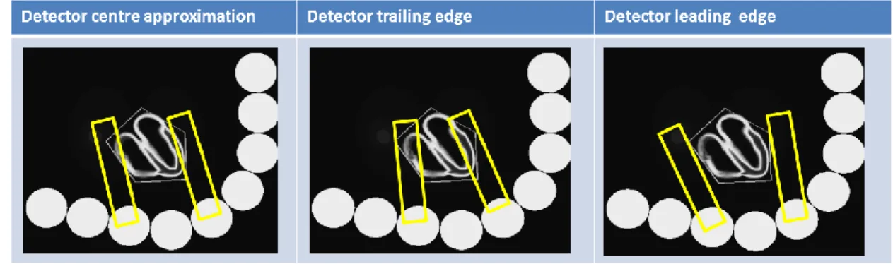
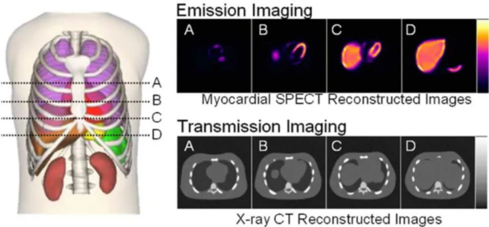
_________________________________________________________________________________ 24 Fig. 2.14. The three different algorithms available in the model simulator used to calculate the scan patterns. _________________________________________________________________________ 24 Fig. 2.15. Anterior view of the 4-D NCAT combined with models of imaging process, the phantom can
simulate emission and transmission imaging data47. _______________________________________ 25
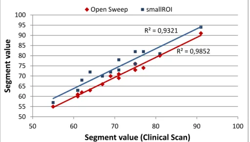
Fig. 3.1. Methodology diagram showing that to obtain the projections, both camera (created in D_SPECT interface) and source (obtained with NCAT phantom program) are needed. Then both are loaded on the simulator interface (zoomed representation of Fig. A in appendix section) in order to calculate the projections. Then projections can be reconstructed and data analyzed. The diagram also shows that different cameras are used while the source is always the same. _____________________ 27 Fig. 3.2. Interface to easily load, create and save ROIs _____________________________________ 28 Fig. 3.3. Transaxial view of the heart A. two different ROI positions, shifting up and left, and B. three different ROI sizes selected for the study, the original, the bigger and a smaller ROI. _____________ 29 Fig. 3.4. Scheme of the four different scan patterns created. For Open sweep the whole FOV is scanned, the Clinical represent the scan pattern performed by D-SPECT clinically, where a ROI is defined and the detectors spend around 60% of the time scanning inside the ROI and the remaining time on the rest of the FOV. ROI only, only the ROI is scanned using detector leading edge algorithm to calculate the projections while for the small ROI the detector trailing edge was the one applied._______________ 31 Fig. 3.5. Clinical transverse, coronal and sagittal views of the LV of the heart for two different scan patterns, taken from AMIDE. The initial ROI represents the ROI where the heart is on the centre of the region and the size of it corresponds to the first simulation. _________________________________ 32 Fig. 3.6. Reconstructed images for four different scan patterns. The left ventricle of the myocardium seems to become thinner from data from left to right. Right ventricle and atria are not visible for the small ROI scan patterns, and there are artefacts around the heart. ___________________________ 33 Fig. 3.7. Bullseye plots obtained from QPS for both clinical open sweep and small ROI. Each segment represented has a value between 1 and 100, given a scale of intensity on that segment. ___________ 33 Fig. 3.8. Three slices of the short axis of the heart view for both open sweep and small ROI. The two extreme slices of short axis were not represented when the projections were calculated with small ROI. _________________________________________________________________________________ 34 Fig. 3.9. Plot of 14 inner rings segment values for open sweep and small ROI scan compared with the
values for each segment of the clinical scan. Respective R2 values are plotted. __________________ 34
Fig. 3.10. Mean activity in the left ventricle of the myocardium selected by a 3D mask based on intensity, for all the four scan patterns (Open sweep, clinical, ROI only, small ROI). _____________ 36 Fig. 4.1. Methodology diagram showing that to obtain the projections, both camera (created in D_SPECT interface) and source (obtained with NCAT phantom program) are needed. Both are loaded on the interface (zoomed representation on Fig. A in appendix section) in order to calculate the projections. Then projection can be reconstructed and data analyzed. The diagram also suggests the camera used is always the same simulating a ROI only scan protocol, while several sources are used for the simulations. ____________________________________________________________________ 37
xi
Fig. 4.2. Axial slice of four phantoms created to simulate different extra-cardiac activities. Coronal view of the phantom is present on the image on the right to show the position of the liver in relation to the heart. The red horizontal line, represent the slice where the other images were obtained. __________ 38 Fig. 4.3. Reconstructed images of the five simulations performed. The extra cardiac activity is visible in all the images. For hs1left data the atria and both ventricles are visible, while for the hs1right the activity sphere is so close that the right ventricle was not reconstructed in the same way. From the left to the right image, the activity on the right ventricle and atria is reduced. All images are scaled to the same maximal value. ____________________________________________________________________ 40 Fig. 4.4. Plot of 14 inner rings segment values the raised liver and the hs1right data compared with the
values for each segment of the reconstructed image with no extra-cardiac activity. Respective R2 values
are plotted after fitting the trendline. ___________________________________________________ 40 Fig. 4.5. Plot of 14 inner rings segment values for raised liver compared with the values for each
segment with no extra-cardiac activity, both without attenuation modelling. R2 values are plotted after
fitting the trendline. _________________________________________________________________ 41 Fig. 4.6. Mean activity in the left ventricle of the myocardium selected by a 3D mask based on intensity, for all the six simulation. The activity is in percentile in relation to the mean activity when no extra-cardiac activity is present. The blue bars represent the results for the simulations performed with attenuation modelling, while the purple bars represent the simulations done without attenuation modelling. ________________________________________________________________________ 42 Fig. 4.7. Images obtain in QPS showing the heart in relation to its own axes. Reconstructed image with no extra cardiac activity with and without attenuation modelling is represented by the short axis (SA), horizontal long axis (HLA) and vertical long axis view (VLA). The same views were obtained for the simulation where the liver was raised, again with and without attenuation modelling. ____________ 43 Fig. 5.1. Methodology diagram showing that to obtain the projections, both camera (created in D_SPECT interface) and source (obtained with NCAT phantom program) are needed. Both camera and source are changed, dependent on the simulation. Then both are load on the model interface simulator in order to calculate the projections. However, the Matlab code of the model interface was modified to simulate a dynamic scan. After reconstructing the projections, the data was analyzed. ____________ 45 Fig. 5.2. Graphical representation of the angular distribution of the 9 detectors over 200 positions. This happens for a dynamic D-SPECT acquisition. The detectors change direction for every 10 positions and the odd and the even detectors scan always in opposite directions. ____________________________ 46
Fig. 5.3. 1 tissue compartmental model used to mimic the TACs obtained clinically on INM. K1 represent
the rate constant from blood pool to myocardium, while k2 = 0. ______________________________ 47
Fig. 5.4. Activity values in relation to time showing two tests performed in order to understand how the NCAT phantom sums the phantoms from two different simulations. Phantom set 1 was created for 3 seconds, each phantom with 0.6 sec. Phantom set 2 was creates from 1.8sec to 3 sec, setting on the text file values from A. 2.4 sec to 3 sec and B from 0 sec to 1.8 sec._______________________________ 48 Fig. 5.5. Initial 8 sec TAC of the blood pool obtained with 3 different simulations with NACT phantom. The value of a pixel in the blood pool of each of the 120 phantom was plot (relative activity) in order to the correspondent time in seconds. _____________________________________________________ 49
xii
Fig. 5.6. TACs for blood pool (bolus injection), liver and myocardium obtained by selecting a pixel values for each organ in 480 different phantoms, simulation a 72 sec scan. _____________________ 50 Fig. 5.7. Diagram of the process used to obtain the simulated dynamic data and the reference data. For each created frame the correspondent 10 phantoms are used to simulate the changes of activity over time. The projections for all 10 positions of the camera are calculated for each phantom, but only the simulated projections calculated with the phantom and the detectors on the right position are chosen. The referenced data used only one phantom to obtain each frame, being that phantom the mean value of the 10 phantoms used in the simulated dynamic data. For the 10 different views, the detectors will always see the same phantom. After the selection of projections the same number of frames is obtained
and the data compared with TACs and K1 values. _________________________________________ 51
Fig. 5.8. Representation of the projections selected to create a 3 sec/frame scan, using the saved projections calculated to create de 1.5 sec/frame scan. The first table represent the available saved projection needed to create the first frame of 1.5sec/frame scan, being associated with camera A. The shadowed columns represent the selected the direct sampling selection while the right symbols represent the selected projection. The second table represent the same but for frame 2 of 1.5 sec/frame, being the camera B associated with the projections. _______________________________________________ 53 Fig. 5.9. Six different injection rates obtained selecting a pixel value on the blood pool of several phantoms. Each curve represents a pixel value on the blood pool for several phantoms, for six different sets of phantoms. Each set of phantom represent different injection rates, from rate 1 (slowest) to rate 6 (faster). __________________________________________________________________________ 55 Fig. 5.10. Diagram representing how the data was organized in order to make a quantitative and qualitative analysis of the resultant reconstructed images. __________________________________ 58 Fig. 5.11. Location of the blood pool and myocardium VOIs (based on intensity) in a slice of the reconstructed data, selected to create TACs. _____________________________________________ 59 Fig. 5.12. Axial slice of the heart for all the frames obtained with the dynamic scan data, for injection rate 3 and scan sampling of 3 sec/frame, over 18 sec (0.3sec * 16frames). The images are scaled to the maximal value of the correspondent frames obtained with the reference data. ___________________ 61 Fig. 5.13. Axial slice of the heart for all the frames obtained with reference scan data, for injection rate 3 and scan sampling of 3 sec/frame, over 18 sec (0.3sec * 16frames). _________________________ 61 Fig. 5.14. Dynamic scan data: Axial slice of all the frames obtained with the 4 scan samplings over 12 seconds for injection rate 3. On the right side are represented the TACs from dynamic data (red) and TACs from reference data (blue) plotted with information from all frames obtained during the scan time, selecting VOIs on both blood pool (input function) and myocardium. _____________________ 62 Fig. 5.15. Reference scan data: Axial slice of all the frames obtained with the 4 scan samplings over 12 seconds for injection rate 3. On the right side are represented the TACs from dynamic data (red) and TACs from reference data (blue) plotted with information from all frames obtained during the scan time, selecting VOIs on both blood pool (input function) and myocardium. __________________________ 63 Fig. 5.16. Dynamic scan data: Axial slice of all the frames obtained with the 4 scan samplings over 12 seconds for injection rate 5. On the right side are represented the TACs from dynamic data (red) and
xiii
TACs from reference data (blue) plotted with information from all frames obtained during the scan time, selecting VOIs on both blood pool (input function) and myocardium. __________________________ 64 Fig. 5.17. Reference scan data: Axial slice of all the frames obtained with the 4 scan samplings over 12 seconds for injection rate 5. On the right side are represented the TACs from dynamic data (red) and TACs from reference data (blue) plotted with information from all frames obtained during the scan time, selecting VOIs on both blood pool (input function) and myocardium. __________________________ 64 Fig. 5.18. Maximum value of the absolute difference between each point of the TACs obtained with dynamic scan data and reference data, for an open sweep scan. The Maximum value is plot for 5 injection rates and respective scan samplings. ____________________________________________ 65 Fig. 5.19. Maximum value of absolute difference between each point of the TACs obtained with dynamic scan data and reference data, for an ROI only scan. The Maximum value is plot for 5 injection rates and respective scan samplings. ___________________________________________________________ 66
Fig. 5.20. The ratio values between the obtained K1 for reference image (referred as K1 average) and
the K1 obtained with dynamic scan , for the 5 injection rates and respective scan samplings. _______ 67
Fig. 5.21. Maximum value of the absolute difference between each point of the TACs obtained with dynamic scan data and reference data, for an open sweep scan, after interpolation of values for 3sec/frame, 6 sec/frame and 12sec/frame. The Maximum value is plot for 5 injection rates and respective scan samplings. ___________________________________________________________ 67 Fig. 5.22. Dynamic scan data: Axial slice of all the frames obtained with the 4 scan samplings over 12 seconds for injection rate 5, simulated with noise. Representation of TACs from dynamic data (red) and TACs from reference data (blue) plotted with information from all frames obtained during the scan time, selecting VOIs on both blood pool (input function) and myocardium __________________________ 68 Fig. 5.23. Reference scan data: Axial slice of all the frames obtained with the 4 scan samplings over 12 seconds for injection rate 5 simulated with noise. Representation of TACs from dynamic data (red) and TACs from reference data (blue) plotted with information from all frames obtained during the scan time, selecting VOIs on both blood pool (input function) and myocardium. __________________________ 69 Fig. 5.24. Maximum value of absolute difference between each point of the TACs obtained with dynamic scan data and reference data in the blood pool, for simulations with noise. The Maximum value is plot for injection rate 2 and 5 and respective scan samplings. ___________________________________ 70 Fig. 5.25. Maximum value of absolute difference between each point of the TACs obtained with dynamic scan data and reference data in the myocardium, for simulations with noise. The Maximum value is plot for injection rate 2 and 5 and respective scan samplings. ___________________________________ 70
1
1 INTRODUCTION
Single photon emission computed tomography (SPECT) is a nuclear medicine technique, allowing the diagnosis of several diseases in the body, derived from physiology and cellular function. To obtain a SPECT exam, a radiopharmaceutical is administered to a patient and 3D images of its distribution in the body is acquired. SPECT is widely use in cardiac studies but the system has some limitations. Thus, for more accurate diagnosis of cardiac function, D-SPECT was created. The system uses a novel detector geometry and a reconstruction algorithm based on maximum likelihood expectation maximization (ML-EM). The new system has 9 pixelated solid state detectors, mounted vertically in 90º geometry (arranged in a curved configuration to conform to the shape of the left side of the patient’s chest), crystals of cadmium zinc telluride and short wide-angle collimators made with tungsten. Each detector rotates around its central axis with a pre-selected angular orientation and in synchrony. D-SPECT also allows a region-centric acquisition. However, before each D-SPECT scan, it is essential to make a quick pre-scan to determine the position of the heart. With that image the ROI, containing the heart, is selected manually. As a consequence, the system calculates a scanning pattern according to the selected ROI, spending more time acquiring data from the region of interest (ROI) and less from other body parts (normal acquisition). In addition D-SPECT also allows very fast dynamic acquisition, what could be an advantage in relation to conventional SPECT systems. Nevertheless, each of the 9 detectors is small and cannot see the whole heart at once, so there is a possibility to create inconsistent projections. The analysis of dynamic nuclear medicine data comprises fitting models to time-activity curves (TACs) generated from ROIs defined on a temporal sequence of reconstructed images.
The objective of this work is to investigate if the new geometry of the D-SPECT camera as well as the innovative region-centric acquisition of the data, can create any problems on the reconstructed images. Static studies were performed in order to start understanding the limitations of the D-SPECT. For instance, factors such as scanning pattern can be altered and may produce different reconstructed images. Different scanning patterns can be obtained by defining different ROIs and choosing different percentiles of time for the detectors to spend scanning the ROI. Defining different algorithms to calculate the scan pattern may also produces changes on the reconstructed images. The presence of a source of activity, near the heart, but outside the ROI, was also studied to verify how it influences the reconstructed images. Since D-SPECT also allows scanning dynamic processes, the fact the radiopharmaceutical activity is changing at the same time the detectors are moving to acquire the data, was also assessed. Different protocols were study changing the temporal sampling to obtain each frame and the rate of the radiopharmaceutical bolus injection.
To investigate the described situations a NURBS-based cardiac-torso (NCAT) phantom was used in combination with a computer simulator tool, specifically design to simulated static D-SPECT acquisitions. Modifications to the simulations had to be made in order to obtain projections obtained by a dynamic acquisition. Then to visualize and analyze the obtained images different programs were used including Matlab, AMIDE and Quantitative Perfusion SPECT (QPS).
2
Relatively to the organization of the thesis, it was divided in five main chapters, including the
Background, three different studies performed, and the General Conclusion, the last chapter of the work.
Each of the three studies is divided in Aim, Materials and Methods, Results and Discussion, and
Conclusion. For a better understanding of the objectives of study and the theory underlined by the image
acquisition process, the Background chapter was divided in five subchapters. In the first subchapter a brief introduction about the SPECT instrumentation is made including information about cardiac SPECT. The way SPECT images are processed in terms of acquiring the data and obtaining projections, as well as the reconstruction process is also explain on the same subchapter. In subchapter two a comparison between D-SPECT and SPECT is done and the process from acquiring the data till the images are reconstructed is explained for D-SPECT. The importance of dynamic SPECT is assessed in another subchapter (subchapter three) where essential information is disclosed in order to clearly understand the kinetic tracer study. In subchapter four the sources that degrade the reconstructed images in nuclear medicine are explain, concerning that for all the simulation some image degradation factors were modelling, so it is important to understand these affects. Further, the D-SPECT simulator is described in subchapter five as well as the computer phantom used to simulate a source. In chapter three the first project is explain, where the effects of different scan patterns are analyzed. Scan without ROI and with different ROI are study in terms of artifacts on the reconstructed images. Chapter four is where the effect of an activity spheres and the presence of a raised liver with higher activity than the heart, outside the ROI is study, again in terms of the effects on the reconstructed images. The content of these last two chapters was presented at the British Nuclear Medicine Society Spring Meeting 2012. The last chapter is where the effects of tracer kinetics are studied. The importance of the study is explained as well as the processing necessary to create simulations essential to understand the best acquisition protocol.
3
2 BACKGROUND
2.1 CONVENTIONAL SINGLE PHOTON EMISSION COMPUTED TOMOGRAPHY
2.1.1 General Concepts of SPECT System
Single photon emission computed tomography (SPECT) is a nuclear medicine technique used to create cross-sectional diagnostic images. As in any other nuclear medicine exam, a radioactive material is injected intravenously, inhaled or ingested by the patient. Nuclear medicine procedures create functional images that are able to pinpoint molecular activity within the body and offer the potential to identify disease in its earliest stages.
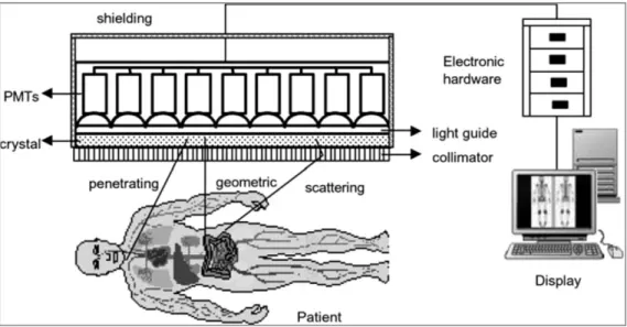
Nowadays, the Anger gamma camera continues to be the main component of SPECT systems. The system consists of one to four cameras mounted on a gantry that rotates around the patient. The basic components of a camera are a collimator, a scintillation crystal and photomultiplier tubes (PMTs), which together form the detector (Fig. 2.1). The gamma camera also includes analogue to digital converter and localisation software1.
Fig. 2.1. Scheme of the principles and basic components of an Anger camera 2.
The collimator is used to mechanically select the gamma photons that are travelling in a specific direction. The most commonly used collimator for SPECT is the parallel-hole collimator that consists of an array of parallel bores with a uniform size separated by septa. Ideally the photons that did not pass perpendicular to the detector will be absorbed. However the collimator will still allow the passage of some photons with a small incidence angle, because the bores cannot be too small. Photons selected by the collimator will fly towards the scintillation detector, and some of them will interact with it, generating an electronic signal. That happens because the energy deposited in the scintillation crystal is converted to visible light photons due to photoelectric effect. That light will propagate till reaching an array of PMTs. The PMTs then will detect the light photons, producing a measurable electric current,
4
that is proportional to the number of the detected photons . Since the objective is to determine the
distribution of the radiopharmaceutical within the body, it is important to know the position of the interaction. That can be found from the light distribution. Then, dedicated electronics and software are used to infer the likely point of impact of the gamma photon based on the output of each PMT in the array.
2.1.2 Image Acquisition and Projections
The acquisition protocols in SPECT have the aim of measuring a sufficient number of projections for tomographic reconstruction. To achieve this, the standard SPECT system has a gantry, where the detectors are attached, which rotates around the patient. The acquisition can be done in different ways: step-and-shoot mode, continuous and continuous step-and-shoot. The most commonly used mode is the step-and-shoot, where the detectors (gantry) move at discrete angles along the circular path.
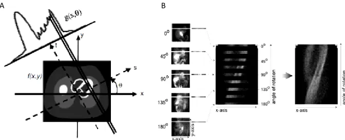
Fig. 2.2. A. Geometry for the 2D image reconstruction problem (adapted from 2). B. Representation of the construction of a sinogram from thin slice of the heart obtained from sample projection views from a 180o acquisition around a patient, the right hand image represents the complete sinogram 1.
As previously mentioned the collimator is used to select the photons so that only those that are parallel to the collimator holes will reach the detector. For each detector angle θ and each location s (s passes perpendicular to the direction of the rays (Fig. 2.2)), the detector is defined by a line given by the equation:
s = x cos θ + y sin θ Eq. 2.1 For a better comprehension of the reconstruction it is important to understand first the projections. Radon defined the projection operator saying that the counts acquired over a specific projection bin, g(s,θ), is the integral of the tracer activity along the line that passes through the object (patient), that is perpendicular to the detector in the case of SPECT. It is mathematically convenient to formulate the problem in terms of the rotated coordinate system (s,t). f(x,y) is the value estimated after the reconstruction, because it gives the number of counts due to the tracer activity 4. Fig. 2.2 describes the 2D geometrical configuration of the reconstruction problem. In this system the origin coincides with
5
the origin in the unrotated (x,y) system and the (s,t) axes are perpendicular and parallel, respectively, to the projection array. After the acquisition of all the projections, they are subdivided by taking all the projections for a single, thin slice of the patient, at a time. All the projections for each slice are then ordered into an image called a sinogram.
The projection operation can be defined as a matrix product given by:
Eq. 2.2
where H is the projection operator, that allows to find the sinogram given the slice, and f and g were already defined. A sinogram is created if the acquired data is rebind in a single plot so that the bin projections are represented on the horizontal axis and the projection angles on the vertical axis. So a sinogram is essentially a stack of the acquired projection views for angles from 0 o to 180o (or 360o). This is applied for the case of SPECT images, where all of the rows in the sinogram came from the same axial (y) position as can be seen in Fig. 2.2. B5.
It is also important to mention that in theory, the Eq. 2.2 can be solved by direct methods. However, due to the noise in the projection, the matrix H is ill-conditioned, so the direct methods are not employed to tomographic reconstruction1.
2.1.3 Tomographic Reconstruction
Since direct methods are not used to solve the Eq. 2.2 to determinate the 3D distribution of the radiotracer from the projections acquired, different methods are applied. Nowadays the reconstructing process can be done using two different approaches in order to solve the referred problem. One can use analytic methods or iterative methods.
2.1.3.1 Analytic Methods
It is possible to visualize the analytical reconstruction considering that the number of photons recorded in any given detector bin, represent the sum of contributions from the activity located along a line perpendicular to the detector surface. That line represents the direction from which the photons originate (in perfect conditions). One way to reconstruct an image is by backprojection, meaning redistribute the collected counts over the contributing individual pixels that lie along the path of the rays in the reconstruction matrix. The activity distribution is obtained if this process is repeated for each projection element and for each angle that is acquired6.
Fig. 2.3. Illustration of star artifact , using 2, 10, 36 and 90 projections equally distributed over 360°. The projections are used
6
Fig. 2.3 shows the reconstructed data from a phantom image (original image in Fig. 2.3 that is obtained with backprojection. The image also shows that, when the number of projections is small in relation to the matrix size, the star artefact is visible.
The backprojection operation, or radon transform can be defined as:
Eq. 2.3
It is important to understand that, the backprojection operation is not the inverse of the projection operation. Applying backprojection to the ray-sums g(s, θ) does not yield f (x, y) but instead, a blurred f(x, y). To overcome this problem, the analytic method used in SPECT is the filtered backprojection (FBP) that consists of filtering the projection data after Fourier transformation of all the acquired angular views4. Then, inverse Fourier transform is computed so that the filtered data can move back to the spatial domain, and after that the backprojection is done to estimate the activity distribution. The filtration step (usually using a ramp filter and a smoothing filter) can be performed prior to or after backprojection. Without the filtering the image will be blurred, due to the summation of crossed lines created during the backprojection process. Although the analytical approaches, to reconstruct images, have high computation speed, they have some flaws. FBP reconstruction amplifies the noise, meaning the statically variation in the number of counts registered, and also because the noise in an individual projection is propagated into a 3D image matrix 1. In addition to this, extra information about collimator geometries or detector placement cannot be taken into account, so if the system uses different geometries than the conventional SPECT, the algorithm cannot be applied, because it assumes angular symmetry of projections. In addition, the FBP also assumes a linear and shift-invariant system. On the other hand, iterative algorithms to reconstruct an image use a more general linear model rather than Radon model, which allows compensation for image blurring and other image degradation effects, such as attenuation, depth-dependence and scatter and also correction of patient motion. It is also important to understand that analytical reconstruction techniques make the assumption that there is -only one solution to the reconstruction problem7. However, in practice, the presence of noise will create a number of possible solutions to the reconstruction problem.
2.1.3.2 Iterative Methods
As in the previous case, the objective is to find the f of Eq. 2.2, but using an iterative algorithm that finds the solution by successive estimation. Unlike the FBP algorithm, in interactive reconstruction, a system matrix that takes into account the probability for each image voxel to have a contribution to a particular projection bin is used. The basic process of iterative reconstruction is to discretize the image into pixels and treat each pixel value as unknown. That system of linear equations can be set up according to the imaging geometry and physics and can be represented, as explained earlier, in a matrix form such as g=Hf.
The matrix H contains the coefficients hij, denoting the probability to detect a photon, emitted from a particular place on the object (emitted from pixel j), on a particular projection bin i such that:
7
Eq. 2.4 The projection space is discrete and the vector g represents the projection data, where each projection is represented by a bin 6. The activity distribution is given by f. Any element of the image, referred to as a pixel, or a voxel, dependent on the dimension of the image. H is a matrix called the
system matrix that describes the imaging process. Attenuation and any linear blurring effect can be
included in the system matrix.
So the problem of reconstruction can be visualized as a way to find the object distribution f, from the measured projections g, as mentioned, but also from information about the imaging system (system matrix) and statistical description of the data and object. But to initialize the process it is essential to create a first estimate of f, usually a uniform image initialized to 0 or 1. Then, based on the estimated activity distribution, f, and taken into account the geometry of the detector and attenuation 7, the first estimation of projection ( ) can be made. Subsequently, the estimated projections ( ) are compared with the measured projections (g). As a consequence, a set of error data is created on the projection space, and used to modify the current estimate, creating a new one. By backprojection these values are mapped to the image space and the estimated activity distribution is updated. These steps are then repeated for each iteration and, with the increasing number of iterations, the reconstruction starts to converge into recognizable images (Fig. 2.4).
Fig. 2.4. Flowchart of a generic iterative
reconstruction algorithm 8
Fig. 2.5. Flowchart of ML-EM iterative reconstruction
algorithm 8.
Nonetheless, from a certain number of iterations the reconstructions increase in noise, so it is important to create a regularization method, stopping the iterations at a certain point before it becomes too noisy9. Moreover, pre- or post-reconstruction smoothing filters can be applied.
8 Fig. 2.6. Example of an iterative reconstruction algorithm applied to a phantom. From left to right, the iteration number is
increasing in each image9.
Nowadays, the more commonly used iterative methods of reconstruction are the maximum likelihood expectation maximization (ML-EM) algorithm and the ordered subsets expectation maximization (OS-EM) algorithm. They are statistical reconstruction techniques, allowing the incorporation of probabilistic models of the noise (as the case of Poisson noise). Nevertheless, these algorithms are mathematically more complex and difficult to solve compared to the Radon transform. As a consequence, and also because these algorithms are iterative, they are more time consuming10. The algorithms need to perform several times projection and backprojection operations, progressively getting closer to the real activity distribution.
The advantages of being a statistical reconstruction, is include a better model of the emission and detection process, the possibility to include a model of statistical noise and also the inclusion of previous information about the distribution that is going to be scanned. The two most used statistical algorithms to reconstruct images are going to be explained in more detail.
2.1.3.2.1 ML-EM
ML-EM algorithm was first demonstrated in 198211, and with the propose of determining the best estimate that can produce the sinogram g with the highest likelihood. Since measurements are subjected to variations due to Poisson phenomena, of radioactive disintegration, the algorithm includes counts statistics through the Poisson law. Therefore, allowing one to predict the probability of a realized number of counts, given the mean number of disintegrations.
In each iteration, the algorithm performs two steps. The expectation step (E or tomography step) and the maximization step (M step). The first step is to determine the expected projections considering the current activity distribution estimation, and the second step is where the image, that has the greatest likelihood to estimate the measured data, is found. When applied to the ET reconstruction, the ML-EM is represented by the following iterative equation, easy to implement and understand:
Eq. 2.5
The factor represent the ratio of the measured number of counts to the current
estimate of the mean number of counts in bin i. On the other hand is the backprojection of that ratio for pixel j.
Since it is an iterative algorithm it is very time consuming and the number of iterations that are necessary to reach the best activity distribution estimation are usually high (require 50–200 iterations), but as previously explained, limited by the noise. The OS-EM was created to speed up this algorithm
9
2.1.3.2.2 OS-EM
OS-EM is an accelerated version of ML-EM and instead of using all the data to obtain an update of the reconstructed images, as the case of ML-EM, each iteration is made after one subset is used. Subsets are small groups of projections data with equally, not contiguous, number of projections. As a result, OS-EM algorithm is just a simple modification of the ML-EM given by the equation:
Eq. 2.6
Using subsets in each iteration, and not all projection, was proved to produce very similar results to ML-EM algorithm, but much faster12. In this case the backprojections are performed just for the projection bins that belong to subset Sn, and in each update a different subset is used. The organization of the subsets is important to the performance of the algorithm. For example, if one subset has stored data from projections number 1, 9, 18, and so on, the data from the following subset could contain data from projections 2, 10, 19 and the same happens for the other subsets6. The application on each subset of
the EM reconstruction is done one by one and so that the resulting reconstruction from subset 1 will be the starting point of subset 2 and so on. Consequently, OSEM converges to the same point as MLEM, but it needs less number of iterations (number of ML-EM iterations divided by the number of subsets).
2.1.4 Cardiac SPECT
SPECT is widely used clinically to diagnose several diseases, including cardiac studies, such as myocardial perfusion imaging (MPI). Most SPECT studies are performed using a conventional dual-head camera, configured in 90o degree geometry to scan the heart, in order to make MPI, taking around 15 to 20 minutes. The time spent for the scanning is necessary to create a good image with adequate statistics, but sometimes artifacts are created due to patient motion13. As previously mention, PMTs are
essential to enhance signal amplitude and the collimator essential to select the photon providing an image with good spatial resolution, however with great cost in sensitivity. The trade-off between resolution and sensitivity determines the performance of conventional gamma cameras. Limitations in sensitivity result in long imaging times and relatively high doses of radiopharmaceuticals.
In order to overcome these problems new cameras dedicated to cardiac SPECT images were created. The collimator design and the reconstructed algorithm were improved and new detectors and gantry geometries arose. One of the created systems is D-SPECT from Spectrum Dynamics (Caesarea, Israel) that allows high-speed perfusion imaging14,15.
2.1.4.1 Myocardial Perfusion Imaging
MPI is the most widely employed non-invasive test used routinely for diagnosing and assessing coronary artery disease (CAD) and other hear diseases, measuring the blood flow16,17. CAD occurs when
arteries become hardened and narrowed, leading to failure of coronary circulation. MPI SPECT images provide a visual 3D image of the perfused myocardium and are usually gated by the electrocardiogram (ECG) in order to make a functional assessment of the images. The radiopharmaceutical must have a property that allows it to distribute in the myocardium, proportionally to blood flow. On the other hand,
10
even though the radiopharmaceutical should be swiftly eliminated, it also has to have a stable retention within the myocardium during the exam time16. To know the relative regional distribution of perfusion, the MPI SPECT can be assessed at both rest and cardiovascular stress (injection of a vasoactive drug), and usually the acquisition is made for both situations18. A region with maximal uptake is assumed to be normally perfused, and regions with significantly reduced uptake are interpreted as abnormally perfused19. Nowadays, the most accepted radionuclide is 99mTc, because it produces images with high quality, resulting from high energy photon (140Kev) with relatively short half-life (6h).
2.1.4.2 Types of Data Acquisition: Static, Dynamic and Gated
SPECT acquisition has been considered to be applied just for static studies. These studies can be seen as long-exposure photography, which means the reconstructed images will represent an average of the radiotracer distribution over the total time of the acquisition. This type of acquisition can only be done when the activity of the radiotracer is nearly constant, or when physiologically induced time variations in the radiotracer distribution are very slow. Static acquisition mode is also performed when the observation of the activity variations is not an important factor.
Besides static protocol, there are two main alternative acquisitions that create a sequence of images that can be viewed as a movie, the dynamic and the gated acquisitions. Even though static images are very useful to obtain perfusion images, little is being done in the last years to improve the basic method of perfusion scintigraphy. No new radiopharmaceuticals were developed nor have new hardware improvements been done. Nevertheless, dynamic cardiac SPECT has emerged as a good option to improve risk stratification of cardiac problems17. Static SPECT acquisition is very important, because myocardium perfusion images can be obtained given information about tracer uptake. However, very useful information about cardiac function can be obtained measuring the tracer uptake over time that will allow the assessment of myocardium blood flow.
Dynamic imaging captures the distribution of a radiotracer over time, revealing information about an organ physiology. Usually are used in visual assessments of organ function and are required for most kinds of kinetic parameter estimation. These parameters describe dynamic behaviour of a tracer in cardiac tissue, giving important clinical information20. This matter will be discussed in more detail in the
section 2.3. Moreover, gated acquisition is a variation of dynamic imaging. Several images of an organ in motion are acquired in synchronism with an electrocardiogram (ECG) signal. The acquired images that started at the same time as the first part of the cardiac cycle are combined to form a composite of all the cardiac cycles. In a similar way, all the successive obtained frames are formed through the combination of all the counts acquired at a correspondent time interval in the cardiac cycle. So in gated SPECT it is assumed a stationary distribution over the entire scan, while for a dynamic SPECT the cardiac motion is typically ignored21.
2.1.5 SPECT Post-reconstruction - Cardiac Image Processing
After the reconstruction process transaxial images are obtained, however if necessary sagittal, coronal and oblique views can also be generated. By convention, the transaxial slices are oriented perpendicular to the long axis of the body. Sagittal and coronal slices are oriented parallel to the long axis of the body and at right angles to each other. This visualization can also be done for cardiac images,
11
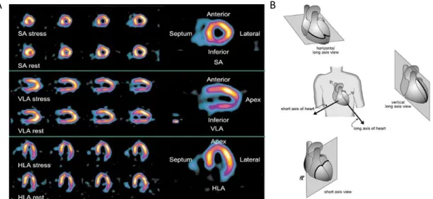
but for a better analysis of MPI images, instead of using the 2D transaxial slices to obtain sagittal or coronal views, it is a common practice to reorient the slices. The axes of the heart can be defined in relation to the heart’s long axis (line from base to apex). The horizontal long axis view (HLA) and vertical long axis view (VLA) are oriented parallel to the long axis of the heart. The short axis (SA) is also used and it is perpendicular to the long axis of the heart. All of these three views are oriented at 90o angles to each other. These are usually used for the examination of coronary blood flow and evaluation of left ventricular function2.
Reconstructed data from MPI SPECT are generally analysed visually, and usually the evaluation is done using images from the described three views, SA, VLA and HLA, from rest and stress studies. In a healthy perfused myocardium, the tracer distribution should be even throughout each slice. No regions of reduce uptake or defects should appear.
Fig. 2.7.A. Standard tomographic slices of the heart representing the short axis (SA), the vertical long axis (VLA) and the
horizontal long axis (HLA) views of the heart16. B. Representation of SA, VLA and HLA in relation to the heart within the body.
Another way to visualize the heart is through a bullseye polar map. This type of visualization allows the quantification of the 3D activity distribution within the myocardium, through the conversion to a 2D polar map. The way the bullseye is made consists in modelling the myocardium into a new system with cylindrical and spherical coordinates. Here the entire LV is displayed as a circular region, with the apex of the ventricle at the centre and the base at the edge. This is then divided in segments (20 or 17 segments) in order to make it possible to compare the heart uptake in different regions of the heart22.
12 Fig. 2.8 On the left side of the image is represented the nomenclature recommended for tomographic imaging of the heart
with bullseye divided in 20 segments. On the right side of the figure, is represented the assignment of the 20 myocardial segments to the left anterior descending (LAD), right coronary artery (RCA), and the left circumflex coronary artery (LCX) 22. This figure was adapted based on information from 23 and 2.
Fig. 2.8 shows the location and the recommended names for the 20 myocardial segments in a bullseye display. The names basal, mid-cavity, and apical are used to identify the location on the long axis of the left ventricle.
2.2 D-SPECT SYSTEM
2.2.1 A Comparison with Conventional SPECT System
The D-SPECT system, specially created for cardiac imaging, has a new design of both photon acquisition system and reconstruction algorithm. The new acquisition system is equipped with 9 pixelated cadmium zinc telluride (CZT) detectors, consisting in 1,024 (16x64) elements, with 5 mm of thickness and a square pixel geometry of 2.46 mm x 2.46 mm, mounted vertically in 90º geometry, arranged in a curved configuration to conform to the shape of the left side of the patient’s chest (Fig. 2.9). It does not contain PMTs, so it is easy to create a compact and flexible design24. The new design also comprises shorter wide-angle collimators made of tungsten, and uses a user selectable centralize region of interest (ROI), as will be explained further on.
It was shown that this design provides an 8 to 10 times higher sensitivity, than a conventional SPECT system, because of the use of wide-angle collimators combines with region-centric data acquisition. It will also have better energy resolution due to the use of CZT, and at the same time the spatial resolution improves 2 times due to the use of resolution modelling during reconstruction26. The improved energy resolution (5.5% at 140 keV) also allows simultaneous application of a dual-isotope protocol with better identification of lesion defect and reduction of photon cross talk6. The OSEM
reconstruction algorithm, based on maximum likelihood expectation maximization method (ML-EM), includes the collimator geometry and compensates for the loss in spatial resolution, due to the shorter collimators that are used in the D-SPECT. Furthermore, the imaging time can be reduced as well as the dose delivered to the patient.