What Makes the Spatial Prisoner’s Dilemma Game Sensitive to Asynchronism?
Carlos Grilo
1,2, Lu´ıs Correia
21Dep. Eng. Inform´atica, Escola Superior de Tecnologia e Gest˜ao
Instituto Polit´ecnico de Leiria
2LabMAg, Dep. Inform´atica, Faculdade Ciˆencias da Universidade de Lisboa
Abstract
We investigate aspects that control the Spatial Prisoner’s Dilemma game sensitivity to the synchrony rate of the model. Based on simulations done with the generalized proportional and the replicator dynamics transition rules, we conclude that the sensitivity of the game to the synchrony rate depends almost exclusively on the transition rule used to model the strategy update by the agents. We then identify the features of these transition rules that are responsible for the sensitiv-ity of the game. The results show that the Spatial Prisoner’s Dilemma game becomes more and more sensitive for noise levels above a given noise threshold. Below this threshold, the game is robust to the noise level and its robustness even slightly grows, compared to the imitate the best strategy, if a small amount of noise is present in the strategy update pro-cess.
Introduction
Spatial evolutionary games are used as models to study, for example, how cooperation could ever emerge in nature and human societies (Smith, 1982). They are also used as mod-els to study how cooperation can be promoted and sustained in artificial societies (Oh, 2001). In these models, a struc-tured population of agents interacts during several time steps through a given game which is used as a metaphor for the type of interaction that is being studied. The population is structured in the sense that each agent can only interact with its neighbors. The underlying structure that defines who in-teracts with whom is called the interaction topology. After each interaction session, some or all the agents, depending on the update dynamics used, have the possibility of chang-ing their strategies. This is done uschang-ing a so called transition rulethat models the fact that agents tend to adapt their be-havior to the context in which they live by imitating the most successful agents they know. It can also be interpreted as the selection step of an evolutionary process in which the least successful strategies tend to be replaced by the most suc-cessful ones.
The discussion about using synchronous or asynchronous dynamics on these models started with a paper by Huber-man and Glance (1993). Synchronous dynamics means that,
at each time step, the revision of strategies happens for all agents simultaneously, while this is not the case for asyn-chronous dynamics. In that paper the authors contested the results achieved by Nowak and May (1992) who showed that cooperation can be maintained when the Prisoner’s Dilemma game is played on a regular 2-dimensional grid by agents which do not remember their neighbors’ past actions. Hu-berman and Glance criticized the fact that the model used in (Nowak and May, 1992) was a synchronous one, which is an artificial feature. They also presented the results of simulations where cooperation was no longer sustainable when an asynchronous dynamics were used. After this work, Nowak et al. (1994) tested their model under several con-ditions, including synchronous and asynchronous dynamics and showed that cooperation can be maintained for many different conditions, including asynchronism. However, the results are presented through system snapshot images, which render it difficult to measure the way they are affected by the modification from synchronous to asynchronous dynam-ics. Recently, in (Newth and Cornforth, 2007), a similar sce-nario was studied using various asynchronous update meth-ods besides synchronous dynamics. The authors found that the synchronous updating scheme supports more coopera-tors than the asynchronous ones.
On the contrary, in (Grilo and Correia, 2007) we found that, in the Spatial Prisoner’s Dilemma game, asynchronous updating supports, in general, more cooperators than syn-chronous updating. This conclusion was only possible be-cause a large number of conditions was tested. Namely, we used small-world networks as interaction topologies so that the whole spectrum between regular and random networks could be explored. We also used the generalized propor-tional transition rule (see Section III), which allows us to tune the level of noise present in the strategy update process. We consider that there is noise when an agent fails to imi-tate the strategy of its most successful neighbor. We found that asynchronous updating is detrimental for cooperation only for very small noise values. That is, for the majority of the noise domain, asynchronous updating benefits coopera-tion. Also, as we go from regular to random networks,
asyn-chronous updating becomes beneficial to cooperation even for very small noise values. In (Grilo and Correia, 2008) we showed that the conclusions do not change if scale-free networks (Barabasi and Albert, 1999) are used. We also showed that the final outcome of the model is basically the same whether a deterministic or a stochastic asynchronous dynamics is used, which is in contrast with results reported in (Gershenson, 2002) for random boolean networks.
The proportion of cooperating agents eventually achieved in a spatial evolutionary game can be influenced by, for ex-ample, the game that is being used, the interaction topology, the transition rule or the update dynamics. The influence of some of these aspects has previously been studied. For ex-ample, in (Pacheco and Santos, 2005) the influence of the interaction topology is examined. Also, in (Tomassini et al., 2006) the influence of the interaction topology, the transi-tion rule and the update dynamics in the Hawk-Dove game are studied.
But, as far as we know, prior to this work, there has been no explanation of the influence of the update dynamics in the outcome of spatial evolutionary games. This work is a step in that direction. Here, we identify the aspects that control the Spatial Prisoner’s Dilemma game sensitivity to asynchronism. Based on previous simulations performed with the generalized proportional transition rule and new ones done with the replicator dynamics transition rule, we first conclude that the sensitivity of the Spatial Prisoner’s Dilemma game to asynchronism depends almost exclusively on the transition rule. We then identify the features of these transition rules that are responsible for the sensitivity of the game.
The paper is structured as follows: in Section II we de-scribe the model used in our simulations. In Section III we first compare the results achieved with the generalized pro-portionaland the replicator dynamics transition rules and then we identify the features of these rules that influence the sensitivity of the model to asynchronism. Finally, in Section IV some conclusions are drawn and future work is advanced.
The Model
The Prisoner’s Dilemma Game
In the Prisoner’s dilemma game (PD), players can cooperate (C) or defect (D). The payoffs are the following: R to each player if they both play C; P to each if they both play D; T and S if one plays D and the other C, respectively. These val-ues must obey T > R > P > S and 2R > T +S. It follows that there is a strong temptation to play D. But, if both play D, which is the rational choice or the Nash equilibrium of the game, both get less payoff than if they both play C, hence the dilemma. For practical reasons, the payoffs are usually defined as R = 1, T = b > 1 and S = P = 0, where b rep-resents the advantage of D players over C ones when they play the game with each other. This has the advantage that
the game can be described by only one parameter without losing its essence (Nowak et al., 1994).
Interaction Topology
We use small-world networks (SWNs) (Watts and Stro-gatz, 1998) as the interaction topology. We build SWNs as in (Tomassini et al., 2006): first, a toroidal regular 2-dimensional grid is built so that each node is linked to its 8 surrounding neighbors by undirected links; then, with prob-ability φ, each link is replaced by another one linking two randomly selected nodes. Parameter φ is called the rewiring probability. Some works (Nowak et al., 1994) allow self-links because it is considered that each node can represent not a single agent but a set of similar agents that may interact with each other. Here, we do not allow self-interaction since we are interested in modeling nodes as individual agents. Repeated links and disconnected graphs are also avoided. The rewiring process may create long range links connecting distant agents. For simplicity, we will refer to interconnected agents as neighbors, even if they are not located at adjacent nodes. By varying φ from 0 to 1 we are able to build from completely regular networks to random ones. SWNs have the property that, even for very small values of the rewiring probability, the average path length between any two nodes is much smaller than in a regular network, maintaining how-ever a high clustering coefficient observed in many real sys-tems including social ones.
Interaction and Strategy Update Dynamics
On each time step, agents first play a one round PD game with all their neighbors. Agents are pure strategists which can only play C or D. After this interaction stage, each agent updates its strategy with probability α using a transition rule (see next section) that takes into account the payoff of the agent’s neighbors. The update is done synchronously by all the agents selected to engage in this revision process. The α parameter is called the synchrony rate and is the same for all agents. This type of update dynamics is called asynchronous stochastic dynamics(Fat`es and Morvan, 2005). It allows us to cover all the spectrum between synchronous and sequen-tial dynamics. When α = 1 we have a synchronous model, where all the agents update at the same time. As α → n1, where n is the population size, the model approaches se-quential dynamics, where exactly one agent updates its strat-egy at each time step.
Asynchronous stochastic dynamics models the fact that, at each moment, more than one agent, but not necessarily all of them, can update their strategy. Usually, asynchronism is understood as sequential dynamics. As an example, in all the works mentioned above, asynchronous dynamics means sequential updating. However, the reality seems to lie some-where between synchronism and sequentiality and, so, both types of dynamics can be considered as artificial. In a pop-ulation of interacting agents, many decision processes can
occur at the same time but not necessarily involving all the agents. If these were instantaneous phenomena we could model the dynamics of the system as if they occurred one after another but that is not usually the case. These pro-cesses can take some time, which means that their output is not available to other ongoing decision processes. Even if we consider them as being instantaneous, the time that in-formation takes to be transmitted and perceived implies that their consequences are not immediately available to other agents. Asynchronous stochastic dynamics also models the fact that, at each time step, the number of agents updating their strategy is not always the same, which is a reasonable assumption. With this type of dynamics, this number fol-lows a binomial distribution with mean α. Apart from these considerations, as we will see in the following sections, the fact that the α parameter allows us to explore intermediate levels of asynchronism is also useful in the analysis of the influence of this feature.
Simulations Setup
All the simulations were performed with populations of 50 × 50 = 2500 agents, randomly initialized with 50% of Cs and 50% of Ds. When the system is running synchronously, i.e., when α = 1, we let it first run during a period of 900 it-erations which, we confirmed, is enough to pass the transient period of the evolutionary process. After this, we let the sys-tem run for 100 more iterations and, at the end, we take as output the average proportion of cooperators during this pe-riod, which is called the sampling period. When α 6= 1 the number of selected agents at each time step may not be equal to the size of the population and it may vary between two consecutive time steps. In order to guarantee that these runs are equivalent to the synchronous ones in what concerns to the total number of individual updates, we let the system first run until 900 × 2500 individual updates have been done. After this, we sample the proportion of cooperators during more 100×2500 individual updates and we average it by the number of time steps needed to do these updates. For each combination, 30 runs were made and the average of these runs is taken as the output.
Simulation Results
In our first simulations (Grilo and Correia, 2007, 2008), we used, a generalization of the proportional transition rule (GP) proposed in (Nowak et al., 1994). Let Gxbe the
aver-age payoff earned by aver-agent x, Nxbe the set of neighbors of
x and cxbe equal to 1 if x’s strategy is C and 0 otherwise.
According to this rule, the probability that an agent x adopts C as its next strategy is
pC(x, K) = P i∈Nx∪xci(Gi) 1 K P i∈Nx∪x(Gi) 1 K , (1) Parameter Values φ 0 (reg.), 1 (rand.), SW: 0.01, 0.05, 0.1 α 0.1, 0.2, 0.3, 0.4, 0.5, 0.6, 0.7, 0.8, 0.9, 1 b 1, 1.1, 1.2, 1.3, 1.4, 1.5, 1.6, 1.7, 1.8, 1.9, 2 K 0, 1/100, 1/10, 1/8, 1/6, 1/4, 1/2, 1
Table 1: Parameter values used in the simulations.
where K ∈ ]0, +∞[ can be viewed as the noise present in the strategy update process. Noise is present in this pro-cess if there is some possibility that an agent imitates strate-gies other than the one used by its most successful neigh-bor. Small noise values favor the choice of the most suc-cessful neighbors’ strategies. Also, as noise diminishes, the probability of imitating an agent with a lower payoff be-comes smaller. When K → 0 we have a deterministic best-neighbor rule such that i always adopts the best best-neighbor’s strategy. When K = 1 we have a simple proportional update rule. Finally, for K → +∞ we have random drift where payoffs play no role in the decision process. For the mo-ment, our analysis considers only the interval K ∈]0, 1]. In this interval the decision process is strongly guided by the payoffs earned by the agents.
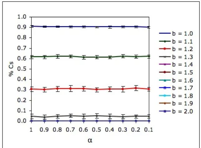
Each simulation is a combination of the φ, α, b and K parameters, and all the possible combinations of the values shown in Table 1 were tested. As Fig. 1 illustrates, when the GP rule is used, in situations where both cooperation and defection coexist, the level of cooperation can change significantly as we change α. For given α and b values, the levels of cooperation may be different when distinct φ and K values are used. Also, the exact way how the model reacts to α changes may change as well. However, no matter the φ and K values used, there is a common qualitative behavior: the model is sensitive to changes in the synchrony rate α. Due to this and space limitations we only show results for φ = 0.1, inside the small world regime.
After experimenting with the GP rule, we also ran simula-tions with one of the most popular transition rules, the repli-cator dynamics rule (RD) (Hofbauer and Sigmund, 1998), which, when used on structured populations, is defined in the following way (Tomassini et al., 2006): the probabil-ity p(sx → sy) that an agent x, with strategy sxand
aver-age payoff Gx, imitates a randomly chosen neighbor y, with
strategy syand average payoff Gy, is equal to:
p(sx→ sy) = f (Gy− Gx) = Gy−Gx b if Gy− Gx> 0 0 otherwise, (2)
where b is the largest possible payoff difference between two players in a one shot PD game. As Fig. 2 illustrates,
Figure 1: % of cooperators for φ = 0.1 and K = 1 (GP rule).
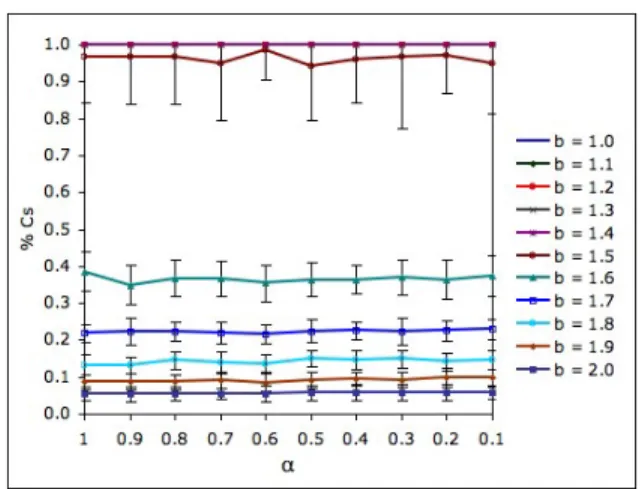
when the RD rule is used, the level of cooperation is ap-proximately constant as we change the synchrony rate α. As for the GP rule, the qualitative behavior of the model does not change no matter the interaction topology used.
Figure 2: % of cooperators for φ = 0.1 (RD rule).
From these results, it follows that the sensitivity of the model to the synchrony rate depends almost entirely on the transition rule that is used. This brings us to the question we try to answer with this work: which features of these transi-tion rules are responsible for the Spatial PD’s game sensitiv-ity to the synchrony rate? After describing the function we use to measure the sensitivity of the model to the synchrony rate, we will start by looking to one of these features: payoff monotonicity.
Sensitivity Measure
We want to measure the sensitivity to the synchrony rate for situations like, for example, the one of Fig. 1, where φ and K are fixed. Let C(φ, R, bi, αj) be the proportion of
co-operators achieved for specific input parameters, where R represents the input parameter set of the transition rule (for example, for the GP rule R = {K}). We first compute, for each b value, the standard deviation of the proportion of co-operators achieved along all α values. We then sum these standard deviations, which gives us the overall sensitivity for a specific combination of φ and R values:
s(φ, R) = 10 X i=0 v u u t 1 10 10 X j=1 (C(φ, R, bi, αj)−C(φ, R, bi))2, (3)
where bi = 1 + 0.1i and αj = 0.1j. This measure
com-presses the results obtained for given φ and R parameters in a single value, which may lead to some loss of information. Therefore, whenever necessary, we will complement the re-sults obtained with equation 3 with an analysis of the data from which the sensitivity values were derived.
Payoff Monotonicity
A transition rule is said to be payoff monotonic if it forbids the imitation of agents with smaller payoffs (Szab´o, 2007). Looking at equations (1) and (2) we easily see that, while the RD rule is payoff monotonic, the GP rule is not (except when K → 0). Given this, we first modified the RD rule in order to turn it into a non-payoff monotonic rule. The modified rule is as follows:
p(sx→ sy) = f (Gy− Gx, M ) = (1 −M1)Gy−Gx b + 1 M if Gy− Gx> 0 1 M − 1 M Gx−Gy b otherwise, (4)
whereM1 is the probability that x imitates y when Gx= Gy.
M ∈ [1, +∞[ can be viewed as the payoff monotonicity de-gree: the bigger M , the smaller the probability that x imi-tates an agent with a lower payoff. We refer to this rule as non-payoff monotonicRD (NPMRD).
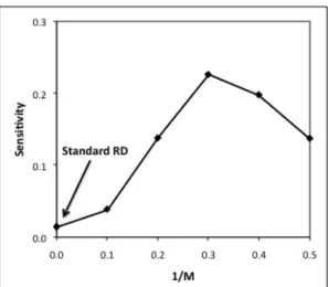
Fig. 3 shows the sensitivity of the model calculated as in equation 3. It shows that the sensitivity grows up to M1 = 0.3 and decreases after this value, although staying higher than the sensitivity of the standard RD rule. This means that the RD rule becomes sensitive to the synchrony rate only if it is non-payoff monotonic. But, if we look at Fig. 4, where the proportion of cooperators is depicted for b = 1, we can see that, for situations where cooperators and defectors coexist, the sensitivity continues to grow even for M1 > 0.3. That is, in these situations the influence of the synchrony rate in the output of the system grows asM1 grows.
After this, we modified the GP rule in order to verify if its sensitivity to the synchrony rate is also due to the fact
Figure 3: Sensitivity of the NPMRD rule to the synchrony rate as a function ofM1 , for φ = 0.1.
Figure 4: % of cooperators for φ = 0.1 and b = 1 (NPMRD).
that agents can imitate a neighbor with a lower payoff. We will refer this rule as payoff monotonic GP (PMGP). Before describing PMGP, we recall that the GP rule takes the sum of the payoffs of C/D agents instead of treating the strat-egy/payoff of each neighbor individually. Putting it another way, the GP rule models a competition between two strate-gies (C and D) so that the winning probability is proportional to the sum of the payoffs of the agents using each strategy. The PMGP rule applies the original GP rule, eq. (1), only if one of the two following conditions is true:
if GCs< GDsand sx= C, (5)
if GCs> GDsand sx= D, (6)
where GCsand GDsare, respectively, the sums of the
pay-offs of C and D neighbors (including the payoff of the agent to be updated x), each one powered to K1. Agent x keeps its strategy if none of these conditions is true.
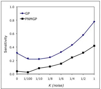
Fig. 5 shows that the PMGP rule becomes much less sen-sitive to α changes than the original version for K > 0.1. Just as an example, compare Fig. 1 with Fig. 6: even taking into account some significant standard deviations in the pay-off monotonic case, the difference in sensitivity between the two situations is clear. The divergence for K > 0.1 means that, above this value, payoff monotonicity also plays an im-portant role in the insensitivity of the GP rule to changes in the synchrony rate, as it does with the standard RD rule. Stating it from the opposite perspective, when agents are al-lowed to imitate less successful strategies, the model’s sen-sitivity grows as this possibility increases. Given that the probability of choosing less successful strategies grows with the noise level, this means that high noise levels increase the model sensitivity to the synchrony rate.
But, Fig. 5 also shows that, for K <= 0.1, the sensi-tivity of the PMGP rule stops diverging from the sensisensi-tivity of the original GP rule. It also shows that payoff mono-tonicity is not the only force that influences the sensitivity of the model to the synchrony rate. Notice that the sensitivity of the PMGP rule also varies as we change the noise level. That is, even when we prevent the imitation of less success-ful strategies, the model’s sensitivity continues to vary with noise: it grows as the noise level decreases. Therefore, there must be another feature related to the noise level that also influences the model’s sensitivity, although less than payoff monotonicity. We address this problem in the next section.
Figure 5: Sensitivity of the GP and PMGP rules to the syn-chrony rate as a function of K, for φ = 0.1.
Figure 6: % of cooperators for φ = 0.1 and K = 1 (PMGP rule).
Imitate the Best Tendency
Given that, with the PMGP rule, agents cannot imitate less successful strategies, what other forces influence the sensi-tivity of the Spatial PD game? If we analyze the original GP rule, we see that the probability of choosing a strategy with a lower payoff becomes very low as K approaches 0. That is, the payoff monotonicity degree increases as K decreases. On the other hand, as K decreases, the tendency to imitate the wealthiest neighbors is increased for both the original and the modified GP rule. Therefore, the two rules become more and more similar as K is decreased. In fact, when K → 0, the two rules become one and the same determinis-tic rule: choose the strategy used by the best neighbor (see Fig. 5). This explains why the the two rules’ sensitivities are similar for K < 0.1.
The above reasoning suggests that, besides payoff mono-tonicity, the “imitate the best tendency” level also influences the sensitivity of the Spatial PD game to the synchrony rate. More specifically, it suggests that the sensitivity of the model increases with the “imitate the best tendency” level. This could explain why the sensitivity of the model slightly in-creases for K values near 0 when the original GP rule is used (see Fig. 5). In order to verify this hypothesis, and given that it is based only on results achieved with the GP rule, we now turn our attention again to the RD rule. The goal is to verify if the ”imitate the best tendency” level also influences the sensitivity of the model when this rule is used. The first modification we have done to the RD rule was to change the way the neighbor y is chosen: each neighbor of the updating agent x has a given probability 0 < θ ≤ 1 of entering a tournament. After this, the wealthiest agent in the tournament is selected and becomes the candidate neighbor y. θ represents the tendency of x to select its best neigh-bors. For example, when θ = 1, y is always the wealthiest neighbor of x.
Once defined the way of choosing y, we still have no to-tal control on x’s “imitate the best tendency”. Notice that, in the standard RD rule, p(sx → sy) only depends on the
difference Gy− Gx. That is, we have no control on the
sen-sitivity of x to the payoff difference between the two agents. Given this, we further modified p(sx→ sy) in the following
way: p(sx→ sy) = f (Gy− Gx, S) = (Gy−Gx b ) 1 S if Gy− Gx> 0 0 otherwise, (7)
where the sensitivity of x to Gy− Gx is given by S ∈
[1, +∞[: for the same payoff difference, the larger S, the bigger the probability that x imitates y. With these two modifications we can cover all the space between the best neighbor rule (θ = 1, S = +∞) and the standard RD rule (θ ≈ |N1
x|, S = 1). We will refer to this rule as extended RD
(ERD).
Fig. 7 shows the sensitivity of the ERD rule calculated as in equation 3. As can be seen in the chart, excepting some small fluctuations, the sensitivity of the model when the ERD rule is used grows as both θ and S are increased. This means that, as for the GP rule, a strong “imitate the best tendency” level also increases the RD’s rule sensitivity to the synchrony rate.
Neighborhood Monitoring
There is yet another feature in which GP and RD differ: while the GP rule models a complete monitoring of the neighborhood (because all the neighbors’ payoffs are con-sidered), the RD rule models a partial neighborhood moni-toring (only the payoff of one neighbor is considered). No-tice that, despite the fact that the above described variant ERD allows a variable neighborhood monitoring, it consid-ers only the payoff of one agent. Thus, we also modified the two rules in order to verify if this feature has some influence on the sensitivity to α.
The GP rule was modified in the following way: each neighbor of x has a given probability β of being ered in equation 1 (the updating agent x is always consid-ered). The β parameter can be viewed as the neighborhood monitoring level. We will refer to this rule as partial neigh-borhood monitoring GP (PNMGP). Fig. 8 shows that the PNMGP rule is less sensitive to the synchrony rate than the original GP rule by a factor of approximately 1/2, main-taing, however, a similar qualitative behavior.
The RD rule was modified so that, as in the case of the original GP rule, the payoff of all the neighbors contribute to the decision of the updating agent x. According to the complete neighborhood monitoringRD rule (CNMRD), the
Figure 7: Sensitivity of the ERD rule for φ = 0.1 as a function of θ and S. θ = |N1
x| means that only a
can-didate neighbor y is randomly chosen as in the standard RD rule. Therefore, the point s(θ = |N1
x|, S = 0)
cor-responds to the sensitivity of the standard RD rule (Fig. 2). s(θ = 1, S = +∞) = 0.312, which is very close to s(K = 0) = 0.314 of Fig. 5. Both points correspond to the best neighbor rule.
probability p(sx → sa) that an agent x, with strategy sx,
changes its strategy to an alternative strategy sa, where sa=
D if sx= C and vice-versa, is equal to:
p(sx→ sa) = GX−GA bkA if GX− GA> 0 0 otherwise, (8)
where GXand GAare the sum of the average payoffs earned
by the neighbors of x playing, respectively, strategy sxand
sa (including x), and kA is the number of neighbors with
strategy sa. Fig. 9 shows the proportion of cooperators
achieved with this rule when φ = 0.1. The sensitivity to the synchrony rate for this situation is equal to 0.030, which is about the double of the sensitivity of the standard RD rule, 0.014, for the same situation (Fig. 2). This result is consis-tent with the one achieved with the PNMGP and GP rules. However, for the two situations, that is, for the GP versus PNMGP and the RD versus CNMRD rules, the difference in sensitivity is partly due to the fact that, with the com-plete neighborhood monitoring versions, there are more b values for which Cs and Ds coexist (compare, Fig. 2 and Fig. 9) than for the partial neighborhood monitoring ver-sions. Therefore, more work must be done, namely explor-ing intermediate levels of neighborhood monitorexplor-ing, in order to determine the real influence of the neighborhood monitor-ing level over the model’s sensitivity to the synchrony rate.
Figure 8: Sensitivity of the PNMGP rule to the synchrony rate as a function of K, for φ = 0.1 and β = 0.1.
Conclusions and Future Work
In this work we identified the features that determine the sensitivity of the Spatial Prisoner’s Dilemma game to the synchrony rate. We first found that the sensitivity of the model depends almost completely on the transition rule used to model the strategy update process. For this, we used the generalized proportionaland the replicator dynamics rules which are, respectively, sensitive and insensitive to the syn-chrony rate no matter the interaction topologies used in the simulations. We then used some variants of these rules in order to identify the features that make them responsible for the sensitivity of the model.
The results can be summarized in the following way: the lower the payoff monotonicity degree and the higher the “imitate the best tendency” level, the more sensitive is the game to the synchrony rate. But, given that these are just consequences of the noise level, we can state the results in the following way: on the one hand, the Spatial Prisoner’s Dilemma game becomes more and more sensitive for noise levels above a given noise threshold (0.1 in the GP transition rule). On the other hand, the game is robust to small noise levels, and its robustness even grows, compared to the im-itate the best strategy, if a small amount of noise is present in the strategy update process. The line corresponding to the original GP rule in Fig. 5 illustrates this well. As far as we know, this is the first time such a result is achieved. We stress that these results are the same for all the interac-tion topologies we used in the simulainterac-tions, which go from regular to random networks.
This result indicates that the noise level may play an im-portant role in the robustness of real dynamical systems where social dilemmas exist. More precisely, it suggests that
Figure 9: % of cooperators for φ = 0.1 (CNMRD rule).
a moderate noise level can enhance the system’s robustness to small variations on the underlying conditions. On the other hand, significant noise levels make a dynamical sys-tem too sensitive to small perturbations. More work must be done, however, in order to verify if this can be generalized to perturbations other than the ones related to the synchrony rate.
Future extensions to this work will explore asynchronous stochastic dynamicswith other games in order to verify if the results achieved with the Prisoner’s Dilemma game can be further generalized. The results achieved in (Tomassini et al., 2006) with the Hawk-Dove game, where the best-neighbor(K → 0), the simple proportional (K = 1) and the replicator dynamicstransition rules, as well as synchronous and sequential updating were used, seem to indicate that, also in this game, the transition rule is what determines the sensitivity of the model. However, only by exploring inter-mediate asynchronism and noise levels we can confirm this. Other transition rules, as the Sigmoid transition rule (Szab´o, 2007) and interaction topologies, as the scale-free network model, will also be explored.
Finally, even if we now know that the noise level of the transition rule is the key feature in what concerns the sen-sitivity of the Spatial Prisoner’s Dilemma game to the syn-chrony rate, we still do not know why it influences the sen-sitivity of the model as it does. Trying to explain this will be one of the main directions of our future work.
Acknowledgements
We thank the reviewers of the paper for their useful com-ments. We also thank the GruVA members Pedro San-tana, Vasco Santos and Luis Sim˜oes for useful discus-sions and comments. This work was partially supported by FCT/MCTES grant No. SFRH/BD/37650/2007.
References
Barabasi, A.-L. and Albert, R. (1999). Emergence of scaling in random networks. Science, 286:509.
Fat`es, N. and Morvan, M. (2005). An experimental study of ro-bustness to asynchronism for elementary cellular automata. Complex Systems, 16(1):1–27.
Gershenson, C. (2002). Classification of random boolean networks. In Proceedings of the Eight International Conference on Ar-tificial Life, pages 1–8. MIT Press.
Grilo, C. and Correia, L. (2007). Asynchronous stochastic dynam-ics and the spatial prisoner’s dilemma game. In Proceedings of the 13th Portuguese Conference on Artificial Intelligence, EPIA 2007, pages 235–246. Springer-Verlag.
Grilo, C. and Correia, L. (2008). The influence of asynchronous dynamics in the spatial prisoner’s dilemma game. In Animals to Animats - 10th International Conference on the Simulation of Behavior (SAB’08). Springer-Verlag. To appear.
Hofbauer, J. and Sigmund, K. (1998). Evolutionary Games and Population Dynamics. Cambridge University Press. Huberman, B. and Glance, N. (1993). Evolutionary games and
computer simulations. Proceedings of the National Academy of Sciences, 90:7716–7718.
Newth, D. and Cornforth, D. (2007). Asynchronous spatial evolu-tionary games: spatial patterns, diversity and chaos. In Pro-ceeding of the 2007 IEEE Congress on Evolutionary Compu-tation, pages 2463–2470.
Nowak, M., Bonhoeffer, S., and May, R. M. (1994). More spa-tial games. International Journal of Bifurcation and Chaos, 4(1):33–56.
Nowak, M. and May, R. M. (1992). Evolutionary games and spatial chaos. Nature, 359:826–829.
Oh, J. C. (2001). Cooperating search agents explore more than de-fecting search agents in the internet information access. In Proceedings of the 2001 Congress on Evolutionary Compu-tation, CEC2001, pages 1261–1268. IEEE Press.
Pacheco, J. M. and Santos, F. C. (2005). Network dependence of the dilemmas of cooperation. Science of Complex Networks: From Biology to the Internet and WWW, CNET 2004, 776:90– 100.
Smith, J. M. (1982). Evolution and the Theory of Games. Cam-bridge University Press.
Szab´o, G. (2007). Evolutionary games on graphs. Phys. Rep., 446:97–216.
Tomassini, M., Luthi, L., and Giacobini, M. (2006). Hawks and doves on small-world networks. Physical Review E, 73(1):016132.
Watts, D. and Strogatz, S. H. (1998). Collective dynamics of small-world networks. Nature, 393:440–442.