PROVIDING AN ACTIVE LEARNING ENVIRONMENT FOR INTRODUCING LINEAR PROGRAMMING
Susana Fernandes1, José C. Pereira1 1
FCT-Universidade do Algarve (Portugal)
Abstract Literature on teaching and learning methods reports strong evidence of the effectiveness of using active learning techniques. This paper presents the GLP-Tool, an example of an active learning technical tool which enables an active learning environment to explore the fundamental concepts of Linear Programming (LP). The GLP-Tool is designed to solve user-defined LP problems with two var-iables, up to a didactical limit of five constraints (plus the non-negativity constraints). Implemented using the computer algebra system Mathematica, this interactive tool allows the user to dynamically explore different objective functions and sets of constraints. All the GLP-Tool functionalities are repre-sented graphically and updated in real time. These interactive, dynamic, and graphical features make the GLP-Tool a powerful tool for teaching and learning LP, both in undergraduate and high school courses. The GLP-Tool is already freely available online at Sapientia - the repository of the “Universidade do Algarve” (University of the Algarve) and at one of the authors’ ResearchGate web page.
Keywords: active learning; graphical linear programming; free, dynamic, interactive, graphical tool.
1 INTRODUCTION
Active learning is generally defined as any instructional approach that engages students in the learning process – as opposed to traditional teaching in which students passively take information from the teacher [1]. The main aspects of active learning are student activity and student engagement in the learn-ing process within the classroom. In an active learnlearn-ing approach the student is called to carry out, in an autonomous (though directed) and reflexive way, activities that lead to the acquisition / construction of new knowledge. In short, active learning requires students to do meaningful learning activities and think about what they are doing. There are several methodologies that fit into an active approach such as the collaborative method, the problem-solving method or the flipped-classroom method. Bonwell and Eison [1] summarises several didactic methodologies that fall within the active learning approach, showing evidence of the value of this approach in the teaching and learning process. Prince [2] examines experi-ences that demonstrate the effectiveness of core elements of the active learning strategies most used in the teaching and learning process of courses in engineering.
When learning mathematical concepts, the use of graphical, dynamic and interactive tools that fumble the connection between algebraic, numerical and graphical representations facilitates the construction of meaning and consequent appropriation of new concepts. In this sense, these tools are in themselves a valuable resource for the construction of a profitable teaching and learning process, but they are of particular importance when used in an active learning environment. Therefore, they are categorised as active learning technical tools. This paper presents the usage of the GLP-Tool, an active learning tech-nical tool for graphical linear programming involving two variables within a context of an active learn-ing environment.
When introducing the subject of Linear Programming (LP) it is rather useful to present the graphical method for solving a two-variable linear program as it provides valuable insights about the general na-ture of multivariable LP models. The graphical method illustrates numerous aspects of the more com-plex, algebra-based, solution algorithm - the simplex method. Specifically, graphically solving a linear program provides students with intuitive visual aids to facilitate their understanding of concepts such as the feasible region, basic feasible solutions, unbounded solutions, binding /nonbinding constraints, de-generacy, slack variables, and so on.
Nonetheless, without a dynamic tool, it is not easy to show students what happens in a (two-variable) LP problem as constraint boundary lines and objective-value lines move around on a graphic plane. To
provide students with an effective learning environment a tool should show graphically and dynamically the construction of the feasible region of two-variable linear programs, and should allow to interactively experiment with the set of feasible solutions and the objective function. So, an active learning technical tool would be most helpful for introducing the subject of LP. In fact, the work of Kydd [3] reports the effectiveness of using such a tool while teaching LP.
We developed the GLP-Tool, a technical tool that engages students and provides them with an effective learning environment. Implemented using the computer algebra system Mathematica, this interactive tool allows the user to dynamically explore and solve two-variable LP problems with different objective functions and constraint sets, and also to intuitively perform post-optimal and sensitivity analysis. All the GLP-Tool functionalities are represented analytically and graphically, and updated in real time. The interactive, dynamic, analytical, and graphical features of the GLP-Tool make this application a powerful tool for teaching LP both in undergraduate and high school courses. It can be used both by teachers to graphically illustrate fundamental concepts and by students to experiment with changes within a graphical representation of a linear program instance, thereby facilitating their understanding of numerous LP concepts.
When setting up to produce an innovative tool for graphical LP, the GLP-Tool, we chose to implement it using the computer algebra system Mathematica [4] not only because it enables the production of sophisticated, dynamic, interactive visual applications but also due to the previous experience of one of the authors in producing didactical tools with Mathematica [5].
The GLP-Tool is freely available online. The reader can download a first version of GLP-Tool at Sapi-entia - the repository of the “Universidade do Algarve” (https://sapientia.ualg.pt/handle/10400.1/2943)
A more recent version is freely available at one of the authors’ ResearchGate web page (https://www.researchgate.net/publication/299559103_GLP-Tool_cdf_file), as of April 2016.
We believe that this new GLP-Tool is an important contribution to the improvement of the teaching and learning process of LP precisely by providing teachers and students alike with an active learning tool to explore fundamental concepts of the subject.
The rest of this paper is organized as follows: section 2 provides a brief introduction to active learning; section 3 presents an overview of existing tools for graphical LP and also presents the motivations for using the computer algebra system Mathematica to produce a new innovative tool; section 4 describes the GLP-Tool concept and explains how to install it and how to use its main features; section 5 provides several usage examples of how to introduce LP concepts with the didactical GLP-Tool in an active learning environment; section 6 describes the presentation of the GLP-Tool to researchers, teachers and students of the operations research community; in section 7 some final remarks are made about our current and future work related with the GLP-Tool.
2 ACTIVE LEARNING: A BRIEF INTRODUCTION
Active learning is generally defined as any instructional approach that engages students in the learning process within the classroom [1]. Many and very different methodologies that include student activity and engagement in the learning process fall into the category of active learning. The work of Bonwell and Eison [1] summarises several of such instruction methodologies.
A very simple technique of active learning reviewed in [1] consists of interspersing the traditional lecture with short (up to two minutes) student activities at about every fifteen minutes. But simply adding ac-tivity to the lecture is not enough. The type of acac-tivity influences how much classroom material is re-tained by the student, as mentioned in [2].
Other simple strategies for active learning include the use of alternative formats for lectures. The feed-back lecture is such a technique which consists of two mini lectures (20 minutes) separated by a study session. In this session students work in small groups while they respond to a question regarding the lecture material. A study guide is provided by the teacher [1].
Many active learning approaches require students to work in small groups towards a common goal, in opposition to learning as a solitary activity. These approaches are called collaborative learning strate-gies. Within these, cooperative learning can be defined as a structured form of group work where stu-dents pursue common goals while being assessed individually. In cooperative learning the focus is on cooperative incentives rather than competitionto enhance learning and to develop social skills like de-cision making, conflict management and communication [1].
Moving further away from the traditional lecture format there is problem-based learning, an instructional method where relevant problems are introduced at the beginning of the course and are used to provide context and motivation for the learning that follows. It usually (but not necessarily) implies collaborative and cooperative learning [1].
Another very different active learning approach is the designated flipped-classroom (or inverted class-room) where students are first exposed to new material outside the class, typically via reading or lecture videos, and then use class time to assimilate that knowledge through problem-solving, discussion, or debates [6]. To help ensure student preparation for class, students are expected to produce work (sum-marizing key concepts, solving problems, answering quizzes, etc.) which is periodically but randomly collected and graded.
Prince [2] examines a number of meta-analyses of the literature on active learning approaches, identifies core elements of the different strategies, analyses the evidences of the effectiveness of each of these core elements in the teaching and learning process and concludes that there is broad support for active learn-ing approaches. Some of the advantages of active learnlearn-ing approaches highlighted in [2] are: introduclearn-ing short student activities into lectures can significantly improve recall of information and extensive evi-dence supports the benefits of student engagement; collaborative learning enhances academic achieve-ment, student attitudes, and student retention; cooperation is more effective than competition for pro-moting a range of positive learning outcomes which include enhanced academic achievement and enhanced interpersonal skills; problem-based learning provides a natural environment for developing problem-solving and life-long learning skills, develops more positive student attitudes, fosters a deeper approach to learning and helps students retain knowledge longer than traditional instruction.
The reader interested in active learning approaches can look into the report “Teaching and learning in active learning classrooms” by Drake and Battaglia of The Faculty Center for Innovative Teaching at Central Michigan University [7] for links and references to definitions and core elements of different strategies, examples of application of specific activities, reports on the impact of the use of these in-struction strategies in students learning outcomes, recommendations to help the teacher prepare for em-bracing active learning approaches and many resources.
With online technological learning tools becoming more popular, readily available and accessible with multiple devices, these tools have increasingly been included into the instructional design of the courses to enhance learning (and also to assess student progress). Technological learning tools are in themselves a valuable resource but they are of most relevance when used in an active learning environment. The GLP-Tool is a technological learning tool for graphical LP involving two variables within a context of an active learning environment. Before describing the GLP-Tool in section 4 we present an overview of existing technological learning tools for graphical LP in the next section.
3 TECHNOLOGICAL LEARNING TOOLS FOR GRAPHICAL LP
There are several Java applets freely available online which graphically solve linear programs. Some of them graphically illustrate the steps of the algebra-based simplex method, moving from one basic solu-tion to the next until it reaches the optimal solusolu-tion(s). Examples of these Java applets are the “Linear Programming and Pivoting in 2D” [8], the “LP Explorer 1.0” [9] or the “Graphical Simplex Algorithm (2D)” [10]. While being very useful when trying to visually explain/understand the simplex method we believe they are not suited for introducing the subject of LP since they do not show very important features in understanding LP as, for instance, the mapping of the objective function value within the set of feasible solutions.
Other Java applets exist that do allow the user to manipulate the constraints and/or the objective function in order to see the effect on the feasible region and on the optimal solution(s). Examples of theses applets are the “Exploring Linear Programming” [11], the “Linear Programming Applet” [12] and the “Ani-mated Linear Programming Applet” [13]. These applets allow the user to define a linear program with two variables with a total number of constraints up to 4 or 5.
GeoGebra is an open source dynamic mathematics software freely available for non-commercial users. It brings together geometry, algebra, spreadsheets, graphing, statistics and calculus in one package. The user can use available GeoGebra resources online or sign in to download offline usable worksheets. The user can also download GeoGebra files (.ggb) or create its own materials after downloading the Geo-Gebra software. By August 2017 the website www.geogebra.org had about one hundred and sixty five materials addressing the theme of LP. Most are slight variations of previously submitted applets. The vast majority of the worksheets available in GeoGebra do not allow the user to dynamically, interac-tively and visually explore any user defined problem instance suited for solving with the graphical method. The one exception is “Linear Programming”[14], available since May 2012, a worksheet by Anthony C. M. OR from the GeoGebra Institute of Hong Kong, and which is an adaptation of the applet “To solve a system of inequations by graph. 02 may 2011”[15] by Michel IROR.
The “Linear Programming” GeoGebra applet [14] allows the user to introduce any LP (or Integer Pro-gramming) instance with two variables and shows its graphical representation – the plotted window of the graphic is resizable (zoom in / zoom out) and movable. Unfortunately inequalities are not plotted as soon as they are introduced. Only the final feasible region is presented and there is no information on which line corresponds to which constraint boundary. With this applet, a change in any coefficient of the constraints requires the user to reintroduce the whole problem instance, thus not allowing to intui-tively perform post-optimal or sensitivity analysis. The “Linear Programming” applet uses a numerical system with finite precision to compute the value of the objective function for any point in the plane. It also allows the user to drag the objective function line and see the way its value changes in the plane. This GeoGebra applet does not however solve the problem instance, so optimal solutions are not visu-ally identified. It is not possible to clearly identify problem instances with one optimal solution, with multiple (limited or unlimited) optimal solutions or unbounded. It also does not give any information when the problem instance is unfeasible.
An intentionally very simple GeoGebra applet is the “Linear Inequalities Slider”[16] by George Ca-diente, available since October 2015, which interactively and dynamically shows that the graph of a linear inequality is a half-plane and that the graph of a system of two linear inequalities is the intersection of the two half-planes. This applet allows the user to interactively change a coefficient of a constraint and updates the correspondent graphical representation in real time.
All Java applets and GeoGebra applets freely available online that graphically solve linear programs are not visually sophisticated when compared to a commercial application. Wolfram's Mathematica is a powerful computer algebra system that enables the production of sophisticated, dynamic, interactive visual applications. Wolfram's Mathematica is used in scientific, engineering, and mathematical fields and in other areas of technical computing. Creating interactive visual models with Mathematica allows users to explore hard-to-understand concepts, test theories, and quickly gain a deeper understanding of the materials being introduced first-hand. In what concerns the work presented in this paper, not only Mathematica algebraically solves LP programs using a single command but also its graphics are com-pletely integrated into its dynamic interactive language. Any visualization can immediately be animated or made interactive using a single command and developed into sophisticated dynamic visual applica-tions.
We have found some Mathematica demonstrations on the website of the Wolfram Demonstrations Pro-ject which address the subPro-ject of LP but none of them works with a user-defined linear program. An intentionally very simple application is the “Graph of Inequalities” [17] which shows that the graph of a linear equation is a straight line, the graph of a linear inequality is a half-plane and that the graph of a system of linear inequalities is the intersection of the half-planes. There's a Wolfram’s Mathematica demonstration that graphically illustrates the steps of the (two-phase) simplex method on randomly gen-erated linear programs - the “Two-Phase Simplex Method” [18]. While being very useful when trying
to visually explain/understand the simplex method we believe it is not suited for introducing the subject of LP.
Some Mathematica demonstrations focus on illustrating the weak version of the fundamental theorem of LP which states that the optimal solution to a linear program, if it exists, is attained at (at least) one vertex of the set of feasible solutions. Examples of these are the “Parametric Linear Programming” [19], the “The Fundamental Theorem of Linear Programming” [20] and the “Graphical Linear Programming for Two Variables” [21]. While being very useful for illustrating the weak version of the fundamental theorem of LP, they do not enable the visualization of very important concepts of LP. Other Mathemat-ica notebooks exist that do allow the user to manipulate the constraints (and the objective function) in order to see the changes on the feasible region and on the optimal solution(s). Examples of these are the “Oil Mallee Farming Optimization Problem” [22] or the “A Simple, Standard Linear Programming Sce-nario” [23].
Another notable product of Wolfram Research is the WolframAlpha internet website (http://www.wolframalpha.com/) which was made available free of charge. WolframAlpha is denomi-nated a computational knowledge engine which can be used to solve a user-defined linear program. When entering a linear program as
Max “objective function” in “(in)equality 1” and “(in)equality 2” and... the engine outputs the optimal solutions(s), the corresponding optimal value and it also graphs the set of feasible solutions, highlighting the feasible solution(s) where the optimal value is reached. WolframAlpha is a powerful engine but it is not an interactive didactical tool. For instance, it does not allow the user to drag the objective function line and see the way its value changes within the feasible region.
In summary, when looking for a graphical tool for introducing LP we found internet freely available tools to be either unfit for this purpose ([8], [9], [10],[15], [16], [18]), misdirected ([19], [20], [21]) or incomplete ([11], [17], [22], [23]). Only three of them ([12], [13], [14]) were flexible enough to enable the visualization of linear programs that either: have an unbounded feasible region; have redundant con-straints; have degenerated solutions; are unbounded; are unfeasible. Unfortunately, we encountered some malfunctions of the “Linear programming applet” [12] when defining totally different instances (namely the ones we will present further on this article). The “Animated linear programming applet” [13] is the only application that actually computes the solution of the problem, but unfortunately it uses a numerical system with finite precision which in some cases leads to errors in the output. Another drawback is the fact that this application has a very poor graphical presentation. The GeoGebra applet “Linear Programming” [14] computes the value of the objective function for any point in the plane (using a finite precision) but it does not compute the optimal solution(s), thus strongly reducing its use-fulness to graphically show/understand important LP concepts.
Running most of the previously described applications (Java applets or WolframAlpha) requires an ex-isting internet connection. Nowadays the internet is globally accessible. Nonetheless, in some situations (some Portuguese high schools, for instance) an application running locally on a personal computer is required. Wolfram's Mathematica demonstrations have the advantage of being built into a single CDF file which runs as a stand-alone application. The user is not required to have the Mathematica program installed. Anyone can just “click” his way through the installation of the free CDF player at the Wolf-ram’s web page (https://www.wolfram.com/cdf-player/) and then download and run any CDF file. For downloading a Java applet the user has to be able to read html or JavaScript code and also be able to find all files needed to build the application. Downloading a GeoGebra’s offline worksheet also implies the download of several directories of files.
With our new tool for graphical LP, the GLP-Tool, we aim at bringing together the best of three worlds: the flexibility of Java applets; the didactical usage of widespread Geogebra worksheets and the sophis-tication and easy packaging of Wolfram's Mathematica demonstrations.
By 2017, some of the applets that were found on the internet when GLP-Tool was created are no longer available, like [10] and [13]. New freely available applications that address the LP subject have appeared
since then, such as the Mathematica demonstration “Graphical Linear Programming for Three Varia-bles” [24] which plots feasible sets for linear problems with three variables, and the web site “PHP Simplex” [25] which illustrates the simplex method. But again, we found the new applications not suited for introducing the subject of LP as they do not allow the user to dynamically and interactively visually explore any user defined problem instance suited for solving with the graphical method.
4 THE GLP-TOOL
The GLP-Tool is a dynamic, interactive and visual tool that allows to solve user-defined LP problems with two variables. In particular, the user can explore different objective functions and constraint sets, obtain graphical and numerical information on optimal solutions and intuitively perform post-optimal and sensitivity analysis.
The GLP-Tool explores the class of LP problems that can be written in the general form, presented in Fig. 1, where the non-negativity constraints are optional.
Fig.1: General formulation of Linear Programs with two variables.
The number of proper constraints is set to a didactical limit of five constraints, plus the non-negativity constraints. This limitation was based on the fact that the GLP-Tool is not a mere calculator but rather an active learning tool designed to engage students and provide them with an effective LP learning environment. With that in mind, we found that the five constraints limit was more than enough to illus-trate all the main LP concepts without cluttering the visual interface of the GLP-Tool. In addition, we could not find in the main literature any instances of graphical LP problems that would exceed the five constraints limit.
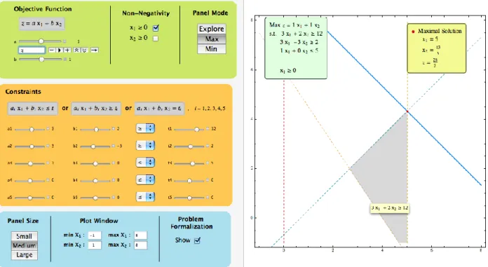
All the functionalities of the GLP-Tool, along with all the displayed information, are designed to con-form to the way LP is used in research and presented in the classroom, both at high school and under-graduate levels. All the GLP-Tool features are represented graphically and updated in real time. A usage example of the GLP-Tool is presented in Fig. 2. Visually, this active learning tool is divided into two main panels.
Left Panel: This panel contains all the controls that allow the user to define the LP problem instances. In addition, it includes some options related with the visual display of the feasible region and the objec-tive function. The user can also choose to visualize the formalization of the problem instance. More importantly, the feature Panel Mode offers three different ways to interact with the right panel: Explore, Max, and Min.
Right Panel: This panel presents all the graphical information concerning the LP problem instance. The feasible region is depicted along with the constraint boundary lines. The objective function line is graphed for a fixed value of z. The feasible solutions corresponding to this value of z are also presented, when they exist. In addition, the problem formulation and the optimal solution information are displayed in two insets when the corresponding options are chosen.
The GLP-Tool has a very intuitive interface that allows even the most inexperienced user with no pre-vious knowledge in educational software to use all the GLP-Tool features in an efficient and autonomous way, right from the start.
Fig. 2: A general usage example of the GLP-Tool. The chosen panel mode is Max. 4.1 Using the GLP-Tool
As mentioned before, all the graphical and analytical information presented in the left and right panels is displayed in real time thanks to the symbolic and numerical computation capabilities of Mathematica. This renders the GLP-Tool as an eminently dynamic tool designed for active learning.
The user can set the values of all the coefficients of a linear problem using the respective sliders. The values can be changed one by one in a discrete or continuous way. In particular, this kind of control allows the automatic continuous change of the coefficient values by clicking the play button (►) de-picted, for example, bellow the a slider in Fig. 2. When choosing this option the user will immediately see an animation of the corresponding graphical information in the right panel. For instance, one may rotate or translate one of the constraint boundary lines and observe how the feasible region changes accordingly. In addition, the corresponding problem formulation can be seen continuously changing when the respective light green inset is displayed in the right panel (see Fig. 2). Note that this inset is not a static display but rather a dynamic object in which all the contained information is updated in real time.
The problem formulation can also be seen in the graphic itself. When the mouse pointer is over a con-straint boundary line a small yellow tag is displayed containing the (in)equality of the corresponding constraint (see Fig. 2). The same is true for the objective function line when graphed for the optimal z. The Panel Mode is one of the main components of the GLP-Tool. This feature includes two optimize modes Max and Min that allow the user to obtain the optimal solution(s) of the respective optimization problems. The optimal information is then displayed both graphically and numerically in the right panel (see Fig. 2). Note that these modes are able to compute all kinds of optimal sets, whether they may be empty, with a single element or with multiple solutions, either bounded or unbounded.
A good usage example of the GLP-Tool is to choose one of the two optimize modes with a fixed feasible region and click the play button for the objective function coefficients a and b. The corresponding line will start rotating and will eventually “visit” several vertices of the feasible region. The user can then observe the optimal solution information change accordingly. This visualization is a very good way to introduce the concept of basic feasible solutions. In addition, it also promotes a better understanding of the role of the objective function coefficients in post-optimal and sensitivity analysis.
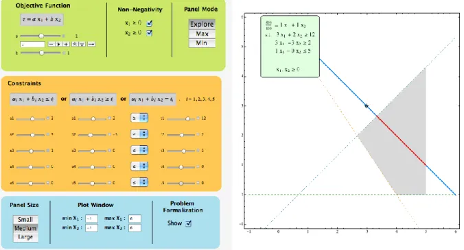
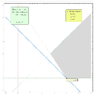
The Panel Mode includes a third mode: Explore. As its name indicates, this option allows the exploration of the set of feasible solutions for any given set of constraints. While in this mode the user can click-and-drag the objective function line across the visible region of the graphic in the right panel. When this line intersects the feasible region the feasible solutions will be highlighted in red (see Fig. 3). At the same time the corresponding value of z is updated within the problem formulation display.
Fig. 3: Using the GLP-Tool to explore the set of feasible solutions. The chosen panel mode is Explore. Another useful feature of the GLP-Tool is the ability to resize the Plot Window (see Fig. 2 and Fig. 3). This functionality is crucial to the visualization of any problem instance, no matter how odd are the coefficient values. To our knowledge there is no graphical LP Java applet with such feature, which seriously reduces their working scope.
We note that the usage descriptions contained in this section are far from being comprehensive. All the GLP-Tool features can be combined to produce a large variety of different useful interactions. As the user becomes more acquainted with this tool, he/she will naturally find those interactions that fit best his/her purpose.
It is also through this kind of dynamic interaction that the GLP-Tool becomes a fully active learning technical tool that engages students and teachers and provides them with an effective teaching and learn-ing environment.
5 INTRODUCING GRAPHICAL LINEAR PROGRAMMING USING THE GLP-TOOL
WITHIN AN ACTIVE LEARNING ENVIRONMENT
In this section we present a didactical use of the GLP-Tool nurturing an active learning environment. We assume that the formulation of linear programs was already discussed and now we want to introduce the graphical method for solving a two-variable linear program.
The GLP-Tool starts by default with a triangular feasible region defined only by the non-negativity constraints and the constraint x1+x21. The teacher may begin the work with the GLP-Tool in the class-room by asking the students to introduce the LP problem instance presented in Fig. 4 into the tool, starting with the constraints.
Fig. 4: Formulation of LP instance (1).
The GLP-Tool dynamically shows the construction of the feasible region as new constraints are added. After all the constraints have been introduced the teacher could question the students to describe the feasible region, identifying some of its solutions. Special attention should be given to the basic feasible solutions. After that if students have still not pointed out that constraint x1≥ 0 is not necessary (the red dashed vertical line does not bound the feasible region in Fig. 3) the teacher may propose that students delete and re-introduce, one by one, each of the constraints of the problem instance and check the changes in the feasible region. Students will then unveil the definition of redundant constraint. The redundancy of constraint x1≥0 can easily be verified by checking and unchecking the corresponding non-negativity option in the left panel and observing that the feasible region in the right panel remains unchanged.
The next step involves setting the values of the coefficients of the objective function. After that, students can use the Explore mode to observe the change in the value of z as the objective function line is dragged across the right panel (see Fig. 3). The teacher can question which feasible solution(s) achieve(s) the optimal value of the problem. By using the Min and Max modes it is possible to actually compute the optimal solutions (4, 0) and (5, 13/3) for the minimum value z = 4 and the maximum value z = 28/3, respectively. This information is displayed in the light-yellow inset in the right panel while the optimal solution is highlighted in the graphic (see Fig. 2).
While in the Max mode, we can also introduce the concept of binding and nonbinding constraints. The students can observe that any change in the independent terms of the inequalities 3x1-3x2≥2 and x15 lead to a different optimal solution. Therefore, these inequalities are binding ones. As for the other con-straints, some variation of the independent terms is allowed before the optimal solution changes (how much variation?) and so, they are considered nonbinding. In particular, the case of the x1≥0 constraint illustrates that all redundant constraints are also nonbinding.
By exploring the tool, students should succeed in finding out how it is possible to change the values of the coefficients either manually (by dragging the slider or by direct input) or automatically (by clicking the play button).
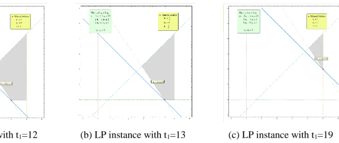
Returning to the initial minimization problem instance (1) presented in Fig. 4, it is possible to introduce post-optimal analysis by questioning the students if the optimal solution would remain the same when the constraint x15 changes to x16. And what about when the constraint 3x1+3x212 changes to 3x1+3x213? After observing the effects of such changes, the teacher should encourage the students to try and modify other independent terms, one at a time. Fig. 5 presents one possible example of this kind of interaction with the GLP-Tool.
(a) LP instance with t1=12 (b) LP instance with t1=13 (c) LP instance with t1=19
Fig. 5: Three similar LP problem instances with different t1 values.
Similarly, sensitivity analysis can be introduced by questioning the students within which interval may the independent term of the inequality 3x1+3x212 vary without changing the set of basic variables in the optimal solution. This concept can then be generalized to include all other coefficients.
As before, the students should modify the values of several coefficients, of binding and nonbinding constraints, and try to determine within which limits the set of basic variables in the optimal solution remains unchanged.
Notice that, when changing the coefficients/independent terms of the inequalities of this problem in-stance, sometimes we will get a feasible region with only one solution while other times we will get an empty feasible region. In this case, an inset is displayed in the right panel stating that the problem is unfeasible, as depicted in Fig. 6.
Fig. 6: Example of an unfeasible LP problem instance.
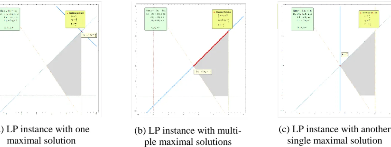
Considering again the initial constraints of problem instance (1) presented in Fig. 4, the students can now perform the sensitivity analysis of the coefficients of the objective function. An interesting usage example in this analysis is to modify the value of the coefficients a and b using the corresponding play button, while on the Max mode. As the values of the coefficients change, the objective function line can be seen rotating in the right panel, moving from one vertex to another adjacent vertex of the feasible region. Also, as depicted in Fig. 7, the information concerning the current maximal solution is displayed and updated in the corresponding inset. The teacher should note that this example clearly illustrates the
11 weak version of the fundamental theorem of LP which states that the optimal solution to a linear pro-gram, if it exists, is attained at, at least, one vertex of the feasible region.
The same example can also be used to introduce the concept of multiple optimal solutions. After ob-serving the motion of the objective function line and looking at Fig. 7(a), (b) and (c), the students should be asked questions such as: When do multiple optimal solutions occur? How many are there? What do they have in common? What makes the values of coefficients a and b in Fig. 7(b) special?
(a) LP instance with one maximal solution
(b) LP instance with multi-ple maximal solutions
(c) LP instance with another single maximal solution Fig. 7: Three similar LP problem instances with different objective function coefficients. Let us now consider the following LP problem instance presented in Fig. 8.
Fig. 8: Formulation of LP instance (2).
As depicted in Fig. 9, LP problem instance (2) presented in Fig. 8 has an unbounded feasible region. Using the Explore mode the students can verify that there is no lower limit for the value of the objective function. Shifting to the Min mode they can then conclude that indeed, the minimization problem is unbounded and no minimal solution can be attained (see Fig. 9 (a)). However, when in Max mode stu-dents will find that the maximization problem is in fact bounded but that the set of maximal solutions is unlimited and corresponds to a ray of the boundary of the feasible region (see Fig. 9 (b)).
12
(a) LP instance with un-bounded solutions set and no minimal solution
(b) LP instance with un-bounded solutions set and multiple maximal solutions
(c) LP instance with un-bounded solutions set and one minimal solution
Fig. 9: Three similar LP problem instances with the same unbounded feasible region.
When introduced for the first time to the notion of unbounded sets of feasible solutions, students tend to believe that this always implies that the LP problem itself is unbounded as in Fig. 9 (a) or that, at the very least, the set of optimal solutions must be unlimited (or maybe just with infinite multiple elements?) as in Fig. 9 (b). In any case, to help clarify the relations between these various notions, it is useful to consider the objective function Min z = x1+x2 for the LP instance (2) presented in Fig. 8. In this case, as depicted in Fig. 9 (c), the LP problem has one single optimal solution (4, 0) corresponding to the minimal value z = 4. The teacher should promote a discussion about the relations between this case and the two previous cases depicted in Fig. 9.
We note that the didactical use of the GLP-Tool described in this section is far from being either the only way of presenting the referred concepts or a comprehensive one. Many more concepts can be in-troduced working with the GLP-Tool, like degeneracy, slack variables, and so on.
6 PRESENTING THE GLP-TOOL TO THE OPERATIONS RESEARCH COMMUNITY
The GLP-Tool was first presented to the Operations Research Community at the EURO|INFORMS MMXIII – 26th European Conference on Operational Research in 2013 [26]. Until the end of the year
2016 there had been 483 downloads of the GLP-Tool at the web site of the repository of the University of the Algarve – Sapientia. The distribution of downloads by country is represented in Fig. 10. Portugal came only in 4th position with 35 downloads, after the United States of America with 176 downloads,
India with 48 downloads and Spain with 39 downloads.
In the year 2017 the team that created the GLP-Tool (and also other graphical, dynamic and interactive tools for the study of functions – the F-Tools [5]) has been visiting higher educational institutions in Portugal, presenting these tools to researchers, teachers and students. These visits are financially sup-ported by the Portuguese “Fundação Caloust Gulbenkian” through the project “Divulgação de Software Educational Dinâmico para uma Aprendizagem Interativa em Matemática no Ensino Superior” (Promo-tion of Dynamic Educa(Promo-tional Software for Interactive Learning in Mathematics in Higher Educa(Promo-tion). This project was funded by the “Fundação Caloust Gulbenkian” upon application to the programme “Projetos Inovadores no Domínio Educativo – Desenvolvimento do Ensino Superior” (Innovative Pro-jects in the Educational Domain – Development of Higher Education). By July 2017 the GLP-Tool was already presented, either in the form of seminars or regular classes, at six different Portuguese higher
13 educational institutions, and also at one national conference and two international conferences held in Portugal.
Fig 10: Top 10 distribution of downloads by country of the GLP-Tool at Sapientia, 2014 – 2016. By the end of the next academic year we intend to conduct a survey on Portuguese higher educational institutions. The aim is to understand if and how the GLP-Tool was used in the courses and how its usage impacted the teaching and learning process, including methods and outcomes of evaluation, in the perspectives of both teachers and students.
7 FINAL REMARKS
This paper presents an innovative tool for introducing graphical LP within a context of active learning methodologies – the GLP-Tool. This dynamic, interactive, visual tool was implemented using the com-puter algebra system Mathematica. The GLP-Tool is available online in the CDF format and it can be used freely as a standalone application by anyone with access to a computer.
When introducing the subject of LP it is rather useful to present the graphical method for solving a two-variable linear program as this method provides valuable insights about the general nature of multivari-able LP models. Nonetheless, without a dynamic tool, it is not easy to show/understand what happens in a LP problem instance as constraint boundary lines and objective-value lines move around on a graphic.
The GLP-Tool is a visual, interactive and dynamic tool where all the analytical and graphical infor-mation is updated in real time. In addition, it allows for user defined data. These features render the GLP-Tool as a fully active learning technical tool that engages students and teachers and provides them with an effective teaching and learning environment.
14
All the functionalities of the GLP-Tool, along with all the displayed information are designed to conform to the way LP is presented in the classrooms, both at high school and undergraduate levels.
Implemented with Mathematica the GLP-Tool brings together the best of both worlds: the flexibility of Java visual applets and the sophistication and easy packaging of Wolfram's Mathematica demonstra-tions.
The GLP-Tool has a very intuitive interface that allows even the most inexperienced user with no pre-vious knowledge in educational software to use all its features in an efficient and autonomous way, right from the start.
In our future work we plan to continue improving the GLP-Tool, including new features such as the visualization of numeric information of the basic feasible solutions and the graphical visualization of the steps of the simplex method.
The GLP-Tool is currently being presented at Portuguese higher educational institutions and used in undergraduate courses. We intend to report on the effectiveness of its use in a near future.
ACKNOWLEDGMENTS
The authors would like to acknowledge the prize awarded to the GLP-Tool by Timberlake-Consultores Lda, the Portuguese branch of Timberlake Consultants, a consultancy service provider which distributes and offers technical support on scientific software packages. The prize was awarded in 2013 at the first International Conference on Algebraic and Symbolic Computation which was held in Lisbon.
The authors would like to acknowledge the Portuguese “Fundação Caloust Gulbenkian” for the spon-soring of the project “Divulgação de Software Educational Dinâmico para uma Aprendizagem Interativa em Matemática no Ensino Superior” (Promotion of Dynamic Educational Software for Interactive Learning in Mathematics in Higher Education) following the application to the programme “Projetos Inovadores no Domínio Educativo – Desenvolvimento do Ensino Superior” (Innovative Projects in the Educational Domain – Development of Higher Education). Within the scope of this project the GLP-Tool has been presented in higher educational institutions in Portugal.
The authors would like to thank the anonymous reviewers for their helpful and constructive com-ments that greatly contributed to improving the final version of t his paper.
REFERENCES
[1] Bonwell, C. C., Eison, J. A., “Active learning: Creating excitement in the classroom”,
ASHEERIC Higher Education Report No. 1, George Washington University, Washington, DC, 1991.
[2] Prince, M., “Does active learning work? A review of the research”, Journal of Engineering Ed-ucation, ASEE, Vol. 93(3), pp. 1-9, 2004.
[3] Kydd, C., “The Effectiveness of Using a Web-Based Applet to Teach Concepts of Linear Pro-gramming: An Experiment in Active Learning”, Transactions on Education, INFORMS, Vol. 12(2), pp. 78-88, 2012.
15 [4] Pereira, J. C., Fernandes, S., “Two-variable Linear Programming: A Graphical Tool with
Math-ematica”, in A. Loja, J. I. Barbosa e J. A. Rodrigues editors, SYMCOMP 2013 - 1st Interna-tional Conference on Algebraic and Symbolic Computation, book of proceedings pp. 159-173, ISBN 978‐989‐96264‐5‐4, Lisbon, Portugal, 2013.
[5] Conceição, A. C., Pereira, J. C., Silva C. M., Simão, C. R. “Mathematica in the Class Room: New Tools for Exploring Precalculus and Differential Calculus”, CSEI2012 - 1st National Con-ference on Symbolic Computation in Education and Research, Lisbon, Portugal, 2012.
http://hdl.handle.net/10400.1/1105
[6] Walvoord, B.E., Anderson V. J., Effective grading: A tool for learning and assessment. San Francisco: Jossey-Bass. 1998.
[7] Drake, E., Battaglia, D., “Teaching and learning in active learning classrooms”. The Faculty Center for Innovative Teaching: Central Michigan University. 2014.
[8] Shepard, B., “Linear Programming and Pivoting in 2D”, The Computational Geometry Lab at McGill, 2010. http://cgm.cs.mcgill.ca/~avis/courses/566/pivoter/main.htm Accessed July 1, 2017.
[9] Hall, J., Baird, M., “LP Explorer 1.0”, University of Edinburgh, 2002. http://www.maths.ed.ac.uk/LP-Explorer/ Accessed July 1, 2017.
[10] Zhang, Y., “Graphical Simplex Algorithm (2D)”, UCMERCED, 2010. https://eng.uc-merced.edu/people/yzhang/ projects/clientsideLP/ Accessed May 21, 2013.
[11] Green, L., “Exploring Linear Programming”, Lake Tahoe Community College, 2010. http://www.ltcconline.net/greenl/java/IntermedCollegeAlgebra/LinearProgramming///Lin-earProgramming.html Accessed July 1, 2017.
[12] Kydd, C., “Linear Programming Applet”, University of Delaware, 2010.
http://www.udel.edu/present/tools/lpapplet/lpapplet.html Accessed July 1, 2017.
[13] Wright, D., “Animated Linear Programming Applet”, St. Edward's University Computer Sci-ences Advanced Computing Lab, 2010. http://www.cs.stedwards.edu/$\sim$wright/linprog/Ani-maLP.html Accessed May 22, 2013.
[14] OR, Anthony C. M., “Linear Programming”, GeoGebra’s worksheet. https://www.geoge-bra.org/material/show/id/9999 Accessed August 1, 2017
[15] IROR, Michel, “To solve a system of inequations by graph. 02 may 2011”, GeoGebra’s work-sheet https:/www.geogebra.org/material/show/id/17 Accessed August 1, 2017
[16] Cadiente, George, “Linear Inequalities Slider”, GeoGebra’s worksheet. https://www.geoge-bra.org/material/show/id/bHkmKCzK Accessed August 1, 2017
[17] Pegg, Jr. E., “Graph of Inequalities”, Wolfram Demonstrations Project. http://demonstra-tions.wolfram.com/GraphOfInequalities/ Accessed July 1, 2017.
[18] Mukherjee, S., “Two-Phase Simplex Method”, Wolfram Demonstrations Project. http://demon-strations.wolfram.com/TwoPhaseSimplexMethod/ Accessed July 1, 2017.
[19] Bunduchi E., Mandric I., “Parametric Linear Programming”, Wolfram Demonstrations Project. http://demonstrations.wolfram.com/ParametricLinearProgramming/ Accessed July 1, 2017. [20] Boucher, C., “The Fundamental Theorem of Linear Programming”, Wolfram Demonstrations
Project. http://demonstrations.wolfram.com/TheFundamentalTheoremOfLinearProgramming/ Accessed July 1, 2017.
16
[21] Carducci, O. M., “Graphical Linear Programming for Two Variables”, Wolfram Demonstrations Project. http://demonstrations.wolfram.com/GraphicalLinearProgrammingForTwoVariables/ Accessed July 1, 2017.
[22] Kragt, M., Jiang, Z., “Oil Mallee Farming Optimization Problem”, Wolfram Demonstrations Project. http://demonstrations.wolfram.com/OilMalleeFarmingOptimizationProblem/ Accessed July 1, 2017.
[23] Boucher, C., “A Simple, Standard Linear Programming Scenario”, Wolfram Demonstrations Project. http://demonstrations.wolfram.com/ASimpleStandardLinearProgrammingScenario/ Ac-cessed July 1, 2017.
[24] Carducci, O. M., “Graphical Linear Programming for Three Variables”, Wolfram Demonstra-tions Project. http://demonstrations.wolfram.com/GraphicalLinearProgrammingForThreeVaria-bles/ Accessed July 1, 2017.
[25] Granja, D. I., Ruiz, J. J. R., “PHPSimplex”, http://www.phpsimplex.com/en/index.htm Ac-cessed July 2017.
[26] Fernandes, S., “Two-variable Linear Programming: A Graphical Tool”, EURO|INFORMS MMXIII – 26th European Conference on Operational Research, Roma, Italy, July 1-4, 2013, book of abstracts, pp. 359, 2013.