University of Algarve
Faculty of Science and Technology
Water circulation pattern in the main channels of
Ria Formosa based on tidal analysis
DELLA PERMATA
Master Thesis of
Erasmus Mundus Master of Science in Eco-Hydrology
Thesis supervised by
Professor Doutor Duarte Nuno Ramos Duarte And
co-supervised by Professor Dano Roelvink
Declaração de autoria do trabalho
Eu Della Permata declaro por minha honra ser a autora deste trabalho, que é original e inédito. Os autores e trabalhos consultados estão devidamente citados no texto e constam da listagem de referências bobliográficas incluída.
Copyright Della Permata. A Universidade do Algarve tem o direito, perpétuo e sem limites geográficos, de arquivar e publicitar este trabalho através de exemplares impressos reproduzidos em papel ou de forma digital, ou por qualquer outro meio conhecido ou que venha a ser inventado, de o divulgar através de repositórios científicos e de admitir a sua cópia e distribuição com objetivos educacionais ou de investigação, não comerciais, desde que seja dado crédito ao autor e editor.
Acknowledgments
First of all, I would like to say grateful to God for giving me such blessful life and health during my study period in Erasmus Mundus of Ecohydrology. Without Him, I am sure I can not finish my study here. Then I would like to say my gratitude to my parents and my brother who always pray and support me whenever I need them and whenever I am down.
Many thanks to Prof. Duarte who have carefully guided me to finish my thesis. Many thanks also to Prof. Dano Roelvink who have been my nice co-supervisor, and Thanks to Prof. Luis Chicharo who accepted me in this Erasmus Mundus Master program. It was really nice experience that I have in my life. Thanks to Prof. Michael McClain who had been my program coordinator during my study period in Delft. Thank you for giving me such a chance to study in Unesco - IHE. My big grateful also want to address to Prof. Flavio Martin who had been my jury during my defense and gave me a lot of suggestions for my thesis. Then many thanks also to Prof. Erik de Ruyter for giving me a lot of encouragement and suggestion during my first two weeks in Delft. And lastly, thanks to all the professors that I can not mention one by one (Prof. Maciej Zalewsky, Prof. Alexandra Chicharo, Prof. Susana Netto, Prof. Alexandra Cravo, Prof. Leo Holthuijsen, and many) for teaching and sharing all the knowledge that you have to all of us. Thanks also to Joanna whom I had been bothering for the administration things in Faro.
Thanks also for all of my ecohydrology friends (Suha, Subham, Kyle, Enrique, Stevo, Teja, Silvia, Raquel, Li, Steffani, Mequan, emeka, Maysa, Thian, and Ashkar). I feel like I have my family here. Thanks for taking care of me, being friend with me, and encouraging me every time I feel down. I will never ever forget the moment that I spend with all of you. Tears and happiness are all together. I will miss you all.
Lastly, I would like to say thanks also to my Indonesian friends, who have been very nice to me (hani; pak eko, mas boy, pak habib, mbak ikha, pak septi, dan semua teman2 PPI portugal; kak upi, kak ira, kak ningsih, kak intan, mbak fatma, kak hesti, tia, renny, gisha, mas nawis, huda, mbak dyah, andri, pak hendiek, dan semua teman2 PPI IHE Delft; dian, melin, sita, bi chan, didi, mbak vivi dan semua anak2 JP4; anak2 kosan KP5A (stella, teteh, etc) thanks a lot...:D)
Abstract
Ria Formosa lagoon, Southern coast of Portugal is considered as a very dynamic system. Current and water level data measurements of tidal dynamic in the main channels of Ria Formosa lagoon had been carried to figure out the hydrodynamic water circulation patterns. The aims of this study in general is to generate a recent hydrodynamic water circulation patterns based on tidal analysis, with the output of tidal dynamic characteristic (tidal propagation, tidal asymmetry and tidal distortion, energy flux and dissipation, water level and velocity longitudinal gradients, phase lag, tidal prisms, water discharge, etc) and residence time, which are used to identify the most suitable areas for seashell to grow.
Several time series of water level and longitudinal component of velocity variations data during completed tidal cicles in the 12 station points of the main channel in Ria Formosa were analyzed using harmonic analysis methods and obtained the average errors of 7.5 % velocity root mean square and 6.75% elevation root mean square, respectively. The tidal analysis results when projected in GIS platform enabled to highlight water circulation patterns in the main channel of Ria Formosa and showed the significance role of Faro-Olhão inlet and Armona inlet in term of energy, volume, and discharge, and less significance role of Sao Luis inlet. The spatial variability of residence time in each stations was obtained and showed that in the west and middle regions of Ria Formosa, a good water exchange were indicated, while in east region, a high residence time magnitude was discovered especially in the inner part of east region with 6.7 days of residence time. This finding result was combined with the average current velocity and maximum flood current and found that Nave Pegos, Culatra, Cações, and Bela Romão stations and adjacent areas are the most suitable area for seashell to grow.
The comparison study between inlet tidal cycle volume and geometric volume calculation was carried out and showed that volume difference represent in average a -38 cm of water level height difference estimation for all lagoon.
The future development of this work will allow introducing a quality level of understanding of the system in Ria Formosa and can give contribution for the fisherman as a preliminary step to find the suitable place for doing seashell aquaculture/ harvesting. Hence, from the Eco-hydrological perspective, the result of this study could be used for the decision maker as a management tool that related to anthropogenic activities such as dredging activity, inlet opening, and other activities that can give impact to the biota life in Ria Formosa.
Keywords : Ria Formosa, Circulation patterns, Tidal analysis, Ecohydrology,
Resumo
O sistema lagunar da Ria Formosa localiza-se na zona costeira Sul de Portugal. Este trabalho teve por principal objectivo estudar os principais padrões de circulação da água nos canais principais, tendo por base leituras de velocidade da corrente e da variação da superfície livre, medidos em vários locais na Ria Formosa. Pretendeu igualmente estudar a propagação e a dissipação de energia da maré, os gradientes longitudinais referentes à variação da superfície livre e à velocidade da corrente, os atrasos da maré em diferentes locais, os prismas de maré, os volumes de água em circulação nos canais principais, os tempos de residência e as potenciais áreas para um melhor crescimento de bivalves tendo por base vários parâmetros hidrodinâmicos. Para o efeito foram medidas série de dados referentes à variação da superfície livre e variação da velocidade na coluna de água, ao longo de ciclos de maré, em 12 estações distribuídas na Ria Formosa, que foram submetidas a uma análise harmónica. Para a componente vertical da maré foram obtidos erros RMS médios de 6.75% e para a componente horizontal de 6.75%. Os resultados obtidos desta análise, quando projectados num sistema SIG permitiram realçar a importância das barras de Faro-Olhão e da Armona na circulação hidrodinâmica deste sistema lagunar em termos energéticos, volume e caudais, bem como uma menor importância relativa por parte da barra de S. Luís. Quando analisados os tempos de residência nas várias estações em estudo, verificou-se que as regiões Central e Oeste da ria foram caracterizadas por uma boa troca de água, enquanto nos sectores mais interiores da região Este por tempos de residência elevados de aproximadamente 6.7 dias. Estes resultados quando conciliados com as respectivas velocidades médias e velocidades máximas de enchente, permitiram definir as estações de Nave Pegos, Culatra, Cações e Bela Romão (e zonas adjacentes) com as mais indicadas para o crescimento de bivalves.
Quando comparados os volumes referentes aos prismas de maré obtidos através das séries de dados maregráficos medidos nas barras em análise, com os prismas de maré geométricos obtidos pela plataforma GIS, constatou-se haver uma diferença entre eles que se materializou numa diferença media da altura da água na laguna da ordem dos -38cm.
Este trabalho para além de contribuir para melhor conhecimento do funcionamento hidrodinâmico da Ria Formosa, e dar um contributo para as associações de mariscadores locais com estes resultados preliminares sobre as melhores localizações para os viveiros de marisco neste sistema lagunar, poderá permitir introduzir em trabalhos futuros outros parâmetros que ajudarão a definir as melhores áreas para a implementação deste viveiros.
Os resultados obtidos neste trabalho no âmbito da Eco-hidrologia, poderão ser usados não só como uma ferramenta de decisão para as entidades locais, mas também dar informações primordiais para a gestão deste sistema costeiro no que diz respeito a actividades antropogénicas, tais como a gestão de trabalhos de dragagem, a abertura de novas barras, e outras actividades que possam ter impactes no Biota da Ria Formosa.
Palavras chave: Ria Formosa, Padrões de circulação, Análise da mare, Eco-hidrologia,
General Index
Declaração de autoria do trabalho ... 1
Acknowledgments ... 2 Abstract ... 3 Resumo ... 5 General Index ... 7 Table Index ... 9 Figure Index ... 10
Acronims and Abbreviations ... 11
1. Introduction ... 12
1.1. Importance of The Subject / Interest of The Subject ... 12
1.2. Thesis Framework / Theoretical Background of The Subject ... 12
1.3. Main objectives and sub-objectives ... 14
1.4. Thesis Structures Descriptions ... 14
2. State of The Art ... 16
2.1. Water level and water flow hydrodynamic ... 16
2.2. Nutrient dynamic ... 17
2.3. Dredging work and open/close inlet ... 18
2.4. Residence time ... 19
3. Study Area ... 21
3.1. Location and Characteristics ... 21
3.2. Climate ... 22
3.3. Hydrodynamics ... 23
3.4. Ecological Functions ... 24
3.5. Social and Economy Importance ... 24
3.6. Water Quality ... 25
4. Methods ... 26
4.1. Field Data ... 26
4.2. Data Treatment ... 28
4.2.1. Raw Time Series ... 28
4.2.2. Harmonic Analysis ... 28
4.2.2.1. Tidal distortion / Tidal asymmetry ... 29
4.2.2.2. Energy Flux and Dissipation ... 29
4.2.2.3. Error Calculation ... 30
4.2.3. Hysteresis Diagram Analysis ... 30
4.2.4. GIS Application ... 31
4.2.4.1. Hydraulic Geometrical Parameters Calculation ... 31
4.2.4.2. Spatial Distribution Performance ... 31
4.2.4.2.1. The mean velocity (ūn,t) in the water column ... 31
4.2.4.2.2. The mean velocity in the channel cross section (<ūn,t>) ... 32
4.2.4.2.3. The mean velocity in the channel cross section during flood and ebb (<ūn>flood and <ūn>ebb) ... 32
4.2.4.2.4. Net Velocity ... 33
4.2.4.2.5. Water Discharge (Qn) and water volume (Vn) ... 33
4.2.4.2.6. Residence Time (RT) calculation ... 33
4.2.4.2.7. GIS performance ... 34
4.2.4.3. Comparison study of tidal inlet volume and annual critical geometry volume of the lagoon ... 36
5. Result and Discussions ... 37
5.1. Harmonic Analysis Fit and Proper test of the data ... 37
5.2. Longitudinal and Temporal gradients of water level and velocity in the main channel ... 44
5.2.1. Longitudinal gradients of water level and velocity in the main channel ... 44
5.2.2. Temporal gradients of water level and velocity in the main channel ... 54
5.2.2.1. For all stations ... 54
5.2.2.2. For inlets ... 58
5.2.2.3. For West Region of Ria Formosa ... 61
5.2.2.4. For middle region of Ria Formosa ... 64
5.2.2.5. For East region of Ria Formosa ... 66
5.3. Volume and Discharge of flood and ebb phase ... 70
5.4. Spatial variability of residence time ... 71
5.5. Preliminary study in determining the suitable area for seashell ponds using Arc GIS ... 73
5.6. Comparison study between inlet tidal cycles volume and geometric volume ... 75
6. Conclusions ... 79
Table Index
Table 4.1. Coordinate location of the stations.. ... 27
Table 4.2. The tidal height (H) and tidal period (T) of the tide in each stations (TP measurement).... ... 28
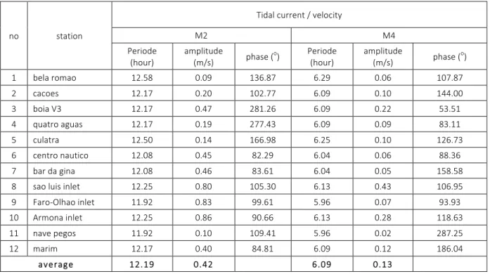
Table 5.1. The tidal velocity amplitude and phase of tidal harmonic constituents M2 and M4 for each stations ... 38
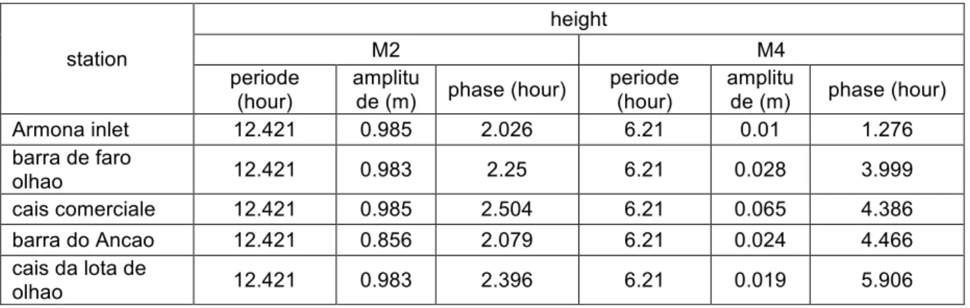
Table 5.2. The tidal height / elevation / water level amplitude and phase of tidal harmonic constituents M2 and M4 for each stations ... 38
Table 5.3. The tidal height / water level amplitude and phase of tidal harmonic constituents M2 and M4 (Baptista, 1987) ... 39
Table 5.4. Root Mean Square calculation ... 39
Table 5.5. Tidal Distortion and Tidal Asymmetry Analysis (amplitude ratio and flood/ebb strength comparison) ... 40
Table 5.6. Flood / Ebb Dominance based on Tidal Phase Period ... 42
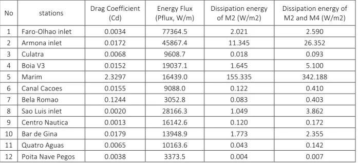
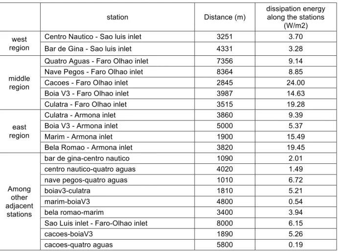
Table 5.7. Tidal energy flux and dissipation for each stations due to M2 and M4 tidal constituent ... 42
Table 5.8. Tidal energy dissipation along the channel stations and the reference distance among the adjacent station in Ria Formosa ... 43
Table 5.9. Water level gradient among adjacent stations at 0 hour, 3 hours, 6 hours, 9 hours and 12 hours. ... 45
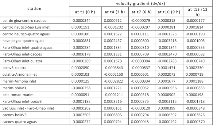
Table 5.10. Velocity gradient among adjacent stations at 0 hour, 3 hours, 6 hours, 9 hours, and 12 hours. ... 45
Table 5.11. tidal amplitude of harmonic analysis and raw data in all stations ... 57
Table 5.12. Phase Lag ... 58
Table 5.13. Phase lag among the inlets in Ria Formosa ... 61
Table 5.14. The slack water for all stations ... 70
Table 5.15. Volume and Discharge of flood and ebb during tidal cycle ... 71
Table 5.16. Inlet tidal prisms during spring and neap tide (Pacheco et al., 2010)...70
Table 5.17. Spatial variability of residence time in all stations ... 72
Table 5.18. Residence Time, Average current velocity, and Maximum Flood Current for each stations in Ria Formosa lagoon... ... 74
Table 5.19 . Inlet tidal cycle volume calculation... ... 76
Table 5.20. The difference estimation between inlet tidal cycle volume and geometrical volume... ... 78
Figure Index
Fig 3.1 Location map of the Ria Formosa System (offshore bathymetry in meters) with location of inlet sections (1–Ancao / Sao Luis Inlet; 2– Faro–Olhao Inlet; 3–Armona Inlet; 4–
Fuzeta Inlet; 5–Tavira Inlet; and 6 – Cacela Inlet). (Dias and Sousa, 2009a). ... .22
Fig 4.1. Tides parameter locations which are currently being measured by MareFORMOSA project, in Ria Formosa (red pins) ... 26
Fig 5.1. Region division in Ria Formosa (West region : Sao Luis inlet, Centro Nautica, Bar de Gina ; Middle region : Faro Olhao inlet, Quatro Aguas, Nave Pegos, Canal Cacoes, Culatra, Boia V3; East region : Armona inlet, Bela Romao, Marim, Boia V3, Culatra). ... 44
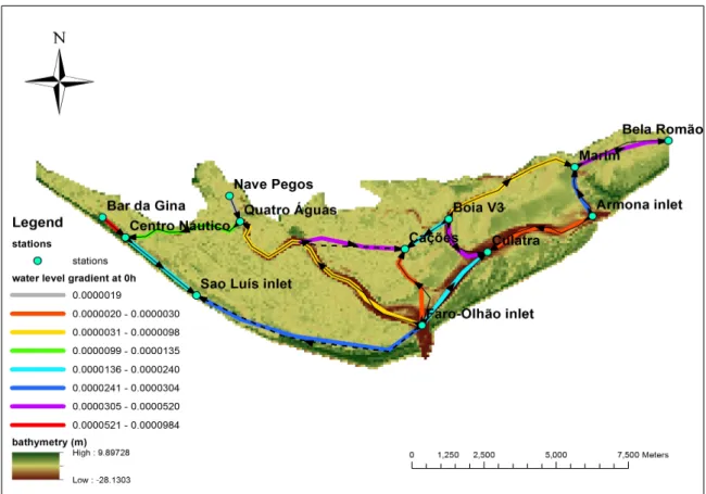
Fig 5.2. Water circulation patterns inside the main channel of Ria Formosa based on water level gradient at 0 hour (at high water in Faro Olhao inlet). ... ...46
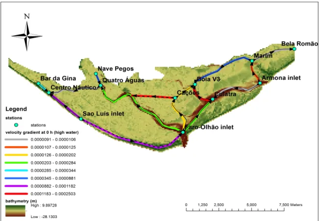
Fig 5.3. The tidal current circulation patterns inside the main channel of Ria Formosa at 0 hour (at high water in Faro Olhao inlet)... ... 47
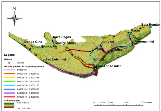
Fig 5.4. Water circulation pattern inside the main channel of Ria Formosa based on water level gradient at 3 hours (at ebbing period in Faro Olhao inlet).... ... 48
Fig 5.5. The tidal current circulation pattern inside the main channel of Ria Formosa at 3 hours (at ebbing period in Faro Olhao inlet)... ... 49
Fig 5.6. Water circulation pattern inside the main channel of Ria Formosa based on water level gradient at 6 hours (at low water in Faro Olhao inlet)... ... 50
Fig 5.7. The tidal current circulation pattern inside the main channel of Ria Formosa at 6 hours (at low water in Faro Olhao inlet)... ... 50
Fig 5.8. Water circulation pattern inside the main channel of Ria Formosa based on water level gradient at 9 hours (at flooding period in Faro Olhao inlet)... ... 51
Fig 5.9. The tidal current circulation pattern inside the main channel of Ria Formosa at 9 hours (at flooding period in Faro Olhao inlet)... ... 52
Fig 5.10. Water circulation pattern inside the main channel of Ria Formosa based on water level gradient at 12 hours (at high water)... ... 53
Fig 5.11. The tidal current circulation pattern inside the main channel of Ria Formosa based on velocity/tidal current gradient at 12 hours (at high water)... ... .53
Fig 5.12. Water level variation for all stations.... ... 55
Fig 5.13. Velocity variation for all stations... ... 55
Fig 5.14. Hysteresis Diagram for all stations... ... 56
Fig 5.15. Water level variation for inlets... ... 59
Fig 5.16. Velocity variation for inlets... ... 59
Fig 5.17. Hysteresis Diagram Analysis for inlets... ... 60
Fig 5.18. Water level variation for west region of Ria Formosa... ... 62
Fig 5.19. Velocity variation for west region of Ria Formosa... ... 63
Fig 5.20. Hysteresis Diagram Analysis for west region of Ria Formosa... ... 64
Fig 5.21. Water level variation for middle region of Ria Formosa... ... 65
Fig 5.22. Velocity variation for middle region of Ria Formosa... ... 65
Fig 5.23. Hysteresis Diagram Analysis for middle region of Ria Formosa... ... 66
Fig 5.24. Water level variation for east region of Ria Formosa... ... 67
Fig 5.25. Velocity variation for east region of Ria Formosa... ... 68
Fig 5.26. Hysteresis Diagram Analysis for east region of Ria Formosa... ... 69
Fig 5.27. Spatial variability of Residence time ... ... 73
Fig 5.28 Spatial variability of Maximum Flood Current (m/s) in Ria Formosa lagoon... .. 75
Fig 5.29 Spatial variability of Average Current Velocity (m/s) in Ria Formosa lagoon... . 75
Fig 5.30 Ria formosa condition during high water level... ... 76
Acronims and Abbreviations
ADP - Acoustic Doppler Current Profiler
ADCIRC - Advance 3-Dimensional Circulation Model GIS - Geographical Information System
IPS - Instituto Portuario do Sul
MOHID - Modelo Hidrodinâmico which is hydrodynamic model in Portuguese RMS - Root Mean Square
SWAT - Soil and Water Assessment Tool TP - Pressure Transducer m - meter m2 - meter quadrat m3 - meter cubic s - second h - hour W - watt
1. Introduction
1.1. Importance of The Subject / Interest of The Subject
This study will carry out the hydrodynamic part of the Ria Formosa lagoon. Since the previous researches in hydrodynamic tend to use established model to describe the Ria Formosa hydrodynamic, this study will treat the data using local approach. It will focus on the recent hydrodynamic water circulation pattern in the main channel based on real data on tidal dynamic analysis and tidal regime within Ria Formosa. Considering that Ria Formosa is a very dynamic system, so using more recent data will be considered convenient (Dias et al, 2009b). The output of this study will be the phase lag of horizontal and vertical component of the tide, tidal dynamic characteristic (tidal asymmetry and tidal distortion, energy flux and dissipation, water level and velocity gradient, tidal prisms, discharge, etc), and residence time, which will be used to identify the most suitable area for seashell ponds. Therefore, this thesis can give contribution for the fisherman to find the suitable place for doing clam aquaculture and clam harvesting. From the Eco-hydrological perspective, the result of this study could give benefit for decision maker as a management tool related to anthropogenic activities such as dredging activity, inlet opening, etc that can give impact to the biota life in Ria Formosa. Besides that, it could help the continuity of the research in order to figure out the next step for researching.
1.2. Thesis Framework / Theoretical Background of The Subject
The purpose of this sub chapter is to provide the reader with the broad theoretical framework used for interpreting the research presented in this thesis on hydrodynamic water circulation pattern in Ria Formosa coastal lagoon in term of barotropic pressure gradient, tidal characteristic (tidal asymmetry and tidal distortion, energy flux and dissipation, water level and velocity gradient, tidal prisms, discharge, etc) and residence time.
Coastal lagoons are shallow water bodies which usually connected to the open sea by one or several tidal inlets between barrier islands (Newton and Mudge, 2003; Dias et al, 2009b) and are classified as inland bodies of water (Schwartz, 2005; Bjorn, 1994). The number and size of the inlets, precipitation, evaporation, and inflow of fresh water affect the condition of the lagoon. Lagoons with little or no interchange with the open ocean, little or no inflow of fresh water, and high evaporation rates may become highly saline (Kusky, 2005). These systems usually run parallel to the coastline, in contrast to estuaries that are normally perpendicular to the coast (Newton and Mudge, 2003; Dias et al, 2009b).
The mean circulation patterns of estuaries and shallow seas originate as the remainder of chaotic first-order flow episodes caused by tides, winds, and river inflow (Csanady, 1976; Reed et al., 2004). Tides are often responsible for the bulk of the kinetic energy present in estuaries. They play a critical role in determining the strength of vertical mixing, can produce significant residual (mean) circulation, and drive lateral circulations within the estuary (Seim et al., 2006). Besides tides, winds, and river inflow, the water circulation is also controlled by rainfall, evaporation, upwelling, eddies, and storms. Water circulation patterns are influenced by vertical mixing and stratification. Vertical mixing determines how much the salinity and temperature will change from the top to the bottom. Vertical mixing occurs at three levels: from the surface downward by wind forces, the bottom upward by boundary generated turbulence (estuarine and oceanic boundary mixing), and internally by turbulent mixing caused by the water currents which are driven by the tides, wind, and river inflow (Wolanski, 2007).
Water circulation patterns can affect residence time and exposure time. The residence time of water is a key variable determining the health of an estuary, particularly from human-induced stresses. Rapid flushing ensures that there is insufficient time for sediment accumulation or dissolved oxygen depletion in the estuary; thus a well flushed estuary is intrinsically more robust than a poorly flushed estuary (Wolanski, 2007). The water residence time can be determined using tidal prism. Tidal prism is the volume of water in an estuary or inlet between mean high tide and mean low tide (Luketina, 1998) or the volume of water leaving an estuary at ebb tide (Davis and Fitzgerald, 2004). If it is known how much water is exported compared to how much of the estuarine water remains, it can be determined how long water reside in that estuary. Tidal prism magnitude can be calculated by multiplying the area of the estuary by the tidal range of that estuary (Davis and Fitzgerald, 2004). During spring or neap tides, when sea level is relatively high and floods back barrier areas that are normally above tidal inundation, the cross sectional area at the entrance of the estuary increases as tidal prism increases (O'Brien, 1931).
If tidal currents at the mouth of an estuary are strong enough to create turbulent mixing, vertically homogenous conditions often develop (Kennish, 1986). In these kind of estuaries, tidal flow is greater relative to river discharge, resulting in a well mixed water column and the disappearance of the vertical salinity gradient. the freshwater - seawater boundary is eliminated due to the intense turbulent mixing and eddy effects. The width to depth ratio of vertically homogenous estuary is large, with the limited depth creating enough
vertical shearing on the seafloor to mix the water column completely. Tidal dissipation has higher values in areas where the tidal currents are stronger, as well as in the areas of transition from the sea to the lagoon (Dias and Sousa, 2009a).
1.3. Main objectives and sub-objectives
The main objective of this study is to present the recent hydrodynamic water circulation pattern inside the main channel based on real data on tidal dynamic analysis and tidal regime within Ria Formosa, with the sub-objectives consist of :
a. Determine the tidal asymmetry and tidal distortion using harmonic analysis fit and proper test.
b. Calculate the energy flux and the energy dissipation of the tide.
c. Establish the spatial and temporal gradients of water level (ɳ) and longitudinal component of velocity (v) in the main channels.
d. Calculate the phase lags of water level (ɳ) and velocity (v) in different stations. e. Calculate the flood/ebb volume and discharge in each stations.
f. Calculate the spatial variability of the residence time in each stations.
g. Determine the suitable area for seashell ponds using Arc GIS considering the average tidal current, maximum flood current, and residence time.
h. Calculate the geometrical water volumes for the lagoon, considering the high water and low water variation/deformation in each stations and conduct comparison study between inlet tidal cycles volumes and the geometrical volumes.
1.4. Thesis Structures Descriptions Chapter 1 : Introduction
Consist of the explanation of the importance of the subject, thesis framework/ Theoretical background of the subject and also the main objectives and sub objective of the study.
Chapter 2 : State of the art
Consist of specific knowledge related to the subject of the study in Ria Formosa and previous researches related to the subject of the study in Ria Formosa lagoon.
Chapter 3 : Study Area
Consist of the detail explanation about the study area such as the location and characteristic, climate, hydrodynamic of the study area, ecological function, social and economy importance, and water quality.
Chapter 4 : Methodology
Consist of the explanation about the methods that are used, the data collection, data treatment, and data analysis method.
Chapter 5 : Result and Discussion
The presentation and explanation about the result of the data treatment and detail analysis discussion.
Chapter 6 : Conclusions
2. State of The Art
2.1. Water level and water flow hydrodynamic
In vertically homogenous estuary, to predict the water circulation pattern, barotropic pressure gradient measurement could be applied. Barotropic pressure gradient is associated with the horizontal change surface elevation according to the hydrodynamic process described by tidal propagation, fresh water of the river inflow, coriolis acceleration, and wind motion, with the influence of the bathymetry (Pacanowski, R. C. And S. M. Griffies, 2000). Barotropic gradient is generated by a sloping sea surface and the pressure gradient is depth
independent. For a fluid that is homogenous (i.e. the fluid's density is constant everywhere)
pressure gradient will only be barotropic. Pressure gradients can also be purely barotropic if the lines of constant pressure (isobars) are parallel to lines of constant density. subsequently a barotropic pressure gradient will not generate vertical shear in the flow, but rather a depth average flow (Ghil et al, 2002).
The tides propagate into the lagoon and altered by its geometry and bathymetry (Dias and Sousa, 2009a). Tidal wave propagates into shallow region, shallow water tides usually increase, include tidal asymmetry (Dias and Sousa, 2009a). Tidal asymmetry of the vertical tide usually refers to the distortion of the (predominant) semi-diurnal tide due to the (quarter-diurnal, sixth diurnal, etc) overtides. The strength of the asymmetry depends on the ratio between the amplitude of the overtide and that of the semidiurnal tide, and the nature of the asymmetry (ebb or flood dominance) is determined by the phase difference between the overtide and the semi-diurnal tide (Wang et al., 1999).
Tidal hydrodynamic related to water level and water flow in Ria Formosa had been simulated using finite element two dimensional model (ADCIRC) (Mendonca, 2001) and using finite difference two dimensional depth-integrated mathematical model (ELCIRC) (Dias and Sousa, 2009a). Both of them used the model to produce the water flow in various inlet and produce water level variations of several station in Ria Formosa which are processed by harmonic analysis to determine the spatial distribution of amplitude and phases of the main harmonic constituents. The harmonic constituents that includes in these two studies are Z0, Msf, O1, K1, N2, M2, S2, MN4, M4, MS4, M6, and 2MS6, which more detail explanation focus on M2, S2, and M4 constituent. The result of these two studies showed the correct representation of tide level, amplitude, and phase of the diurnal and semidiurnal constituent with small error. The semidiurnal constituent have highest amplitude, followed by diurnal (Dias and Sousa, 2009a). In most places, the semidiurnal components are dominant (Van rijn, 1990). The result for M2 can be considered representative of the tide in Ria
Formosa lagoon, since it has most of tidal energy (Dias and Sousa, 2009a). The constituent non linear (M4) has been carried out and showed that the greater velocity gradient at the site, the more significant amplitude in relation to depth (Mendonca, 2001).
Besides that, the result also showed the location of flood dominance areas in Ria Formosa which are in Ancao, Armona, Fuzeta, and Cacela inlet, while ebb dominance areas occur at other inlets (Dias and Sousa, 2009a). This finding is different with the finding of Salles et al (2005) for the Ancao and Armona inlets. This is due to the fact that the duration of flood and ebb is not a determinant factor for flow dominance. Longer duration of the flood (ebb) may be associated with flood (ebb) dominance, due to the existence of strong residual circulation between inlets. In fact, the larger flood (ebb) discharge in a shorter period does not lead to stronger flood (ebb) currents (Dias and Sousa, 2009a). So it means that the discharge and the period of the ebb or flood need to be taken into consideration for determining the flow dominance.
Other similar work has been conducted by Martins et al (2003) using a model which is developed by Portuguese researchers, MOHID, to characterize the system and to understand the processes in Ria Formosa. The hydrodynamic model was forced by the tide at the open boundary and average climatological winds without considering the freshwater flow due to the low and intermittent run off to the system (Gamito, 1997; Coelho et al., 2002; Martin et al, 2003; Serpa et al., 2007). This model was calibrated and validated using local measurement and the result showed a good agreement between the model and the measured data, with small error.
2.2. Nutrient dynamic
Hydrodynamic model is the first step in future studies on water quality, sediment transport, and other studies in the system (Mendonca, 2001). The study of nutrient dynamic inside Ria Formosa correspond to land drainage, waste water treatment plant, and water exchanges across the lagoon inlet had been conducted using SWAT model with Eco-Dynamo model to provide physical-biogeochemical model (Duarte et al., 2008). Ria Formosa is a shallow coastal lagoon with high productivity (Falcao and Vale, 2003). One of the sources that contribute largely for the lagoon water nutrient enrichment (ammonium and phosphate) is the bottom sediment (Serpa et al., 2007).
2.3. Dredging work and open/close inlet
The acquisition of a series of topo-bathymetric surveys and oblique aerial photos (Sedimentary dynamics) had been carried out at Ancao Inlet since its artificial opening in June 1997 until for two years ahead (Vila-Concejo et al., 2003). Six years after this study, the numerical modeling of the impact of the Ancao inlet relocation has also been conducted in Ria Formosa, Portugal (Dias et al, 2009b). This research discussed on the effect of Ancao inlet relocation to the hydrodynamic pattern such as water circulation and the potential pathways of tracers in the western part of Ria Formosa in two distinct configurations: before and after the Ancao Inlet relocation by using numerical modeling method which are hydrodynamic ELCIRC and VELA/VELApart. The hydrodynamic simulation of Ria Formosa was performed using the two dimensional depth-integrated model ELCIRC which uses finite volume / finite difference Eulerian-Lagrangian algorithm and the simulation of the tracers transport was performed with the models VELA and VELApart, with the objective of studying the dispersion of tracers (VELA) and to evaluate the residence times (VELApart). The hydrodynamic model was successfully calibrated and validated against elevation, velocity, and inlet discharge data with result the relocation of Ancao inlet increases the stability of the Ria formosa lagoon: the magnitude of tidal currents, residual velocities, and tidal prism across the bar. The tracers transport simulations showed enhanced water exchanges through the Ancao Inlet and smaller residence times in the western part of Ria Formosa with the present configuration. Overall, it is concluded that the Ancao Inlet relocation had a positive contribution towards increasing the water renewal of the western part of the lagoon, thus decreasing its vulnerability to pollution (Dias et al, 2009b). This study shows that the inlet enlargement and deepening was a successful strategy, and therefore may be implemented to improve the water quality and circulation in other lagoons or estuaries, after the numerical modeling study of possible impacts (Dias et al, 2009b).
The study of inlet dredging in Faro channel also had been carried out by Pacheco et al. (2006). This study aims to study the volumetric evolution of a navigable channel, defining both erosion and accretion sectors and to compare the natural and anthropogenic processes by comparing the three bathymetric maps from the Faro channel (1985, 1994, and 2001) provided the definition of erosive and accumulative sectors and allowed the calculation of the total variation (m3) for each sector. The comparison with the values from the dredging activities in the study area given by IPS (2001) was undertaken to define the concept natural changes and anthropogenic dredging. The result of this study showed the erosion found during the period 1984-1994 is mainly related with dredging activities, while during the
period 1994-2001, both natural and anthropogenic occurred strongly.
2.4. Residence time
Residence time in Ria Formosa had been an object of researches since a long time ago. Duarte et al. (2005 and 2008) did a research on hydrodynamic modeling of Ria Formosa with Eco-dynamo using two dimensional vertically integrated hydrodynamic model based on finite difference method and a semi implicit resolution scheme. Water residence times were estimated by ‘‘filling’’ the lagoon with a conservative tracer and running the model until its ‘‘washout’’ to the sea. The result showed water residence considering a 90% washout range from less than one day near the inlet to more than two weeks at the inner area, with an average values of 11 days. Besides that, the result also showed that Faro - Olhao and Armona inlets give dominant contribution for the lagoon-sea water exchanges and the variability in water residence time at different areas of the lagoon (Duarte et al., 2005 and 2008). These result is relevant with the research done by Ana Mendonca (2001) which also indicates the good water exchange in Ria Formosa by showing the result of ebb velocity is much greater than flood velocity. Since higher ebb velocity than flood velocity means much water transfers outside the lagoon than goes inside the lagoon, so there is more new water transfer inside Ria Formosa lagoon. Finite Element Methods was used to simulate the hydrodynamic pattern of Ria Formosa and tidal current velocities as well as the relationship between semidiurnal harmonic constituent M2 and non linear harmonic constituent M4 were used to predict the ebb/flood dominance (Mendonca, 2001). In contrast to the result of these two researches, Mudge et al. (2008) found that the residence time in the inner regions of Ria Formosa is quite long, so the management models should take into account additional complexities that might arise from the much longer exchange rates of the inner lagoon (Mudge et al., 2008). Mudge et al. (2008) estimates the residence time in Ria Formosa using salinity tracers by comparing the salinity measured during tidal cycle outside and inside the lagoon, and near the outlet of the lagoon. Calculation of the residence time was based on box model worked by Hearn and Robson (2002). This change became zero in lagoons, such as the Ria Formosa in summer, where there was no freshwater inflow. Therefore, increases in salinity above that of the inflowing sea-water were due to evaporation of surface water and the length of time the water was in the system (Mudge et al., 2008).
Besides that, Mudge et al. (2007) also did a research in the relationship between water residence time and oxygen saturation in a mesotidal lagoon, Southern Portugal during summer months where there is no significant freshwater input and has high evaporation rate.
The result showed a significant linear decrease in the oxygen saturation with the increasing residence time in response to discharges of high organic carbon content wastes and potentially eutrophic phytoplankton blooms.
3. Study Area
3.1. Location and Characteristics
Ria Formosa is a shallow coastal mesotidal barrier lagoon, which located in the southern coast of Portugal (36o58' N, 8o02' E to 37o03' N, 7o32' W) (Gamito, 1997; Coelho et al., 2002; Newton and Mudge, 2003; Duarte et al., 2008; Dias et al, 2009b; Brito et al., 2011; Guimaraes et al., 2012). It has large intertidal areas and has mean depth of approximately 3.5 m (Falcao and Vale, 2003; Nobre et al., 2005; Duarte et al., 2008; Brito et al., 2011). Based on the general explanation above, Ria Formosa can be classified as vertically homogenous estuary because of its shallowness (Gamito, 1997; Coelho et al., 2002; Newton and Mudge, 2003; Duarte et al., 2008; Mudge et al., 2008; Dias et al, 2009b; Brito et al., 2011; Guimaraes et al., 2012).
The Ria Formosa basin has an area of 864 km2, it includes 145.22 km2 of wetland as well as 40 km2 of salt extraction ponds, marine culture ponds, salt marsh, exposed sands, navigable channel and mud banks. The salt marshes are composed of silt and fine sand and are intersected by a high density of shallow meandering tidal creeks. The navigable channels were extensively dredged during the year 2000. The average depth of the navigable channels is 6 m although most areas are less than 2 m deep (Salles et al., 2005; Dias et al., 2009b). There are a further 25 km2 of sand dunes, farmland, forest and urban land also in Ria Formosa.
Seaward, it is limited by a non continuous belt of sandy dunes formed by two peninsulas and five barrier islands that separate the lagoon from the Atlantic ocean (Coelho et al., 2002; Dias et al., 2009b; Guimaraes et al, 2012). Ria Formosa has six inlets, which are from west to east: Ancao/Sao Luis Inlet, Faro-Olhao inlet, Armona Inlet, Fuzeta Inlet, Tavira Inlet and Cacela Inlet (Fig. 3.1) (Coelho et al., 2002; Dias et al., 2009b; Guimaraes et al, 2012), where the water exchange between the lagoon and the sea takes place (Dias et al. 2009b; Brito et al., 2011). Among these inlets, Faro-Olhao inlet has been artificially consolidated by two breakwaters. In 1997, the Ancao Inlet, located on the western part of the lagoon, was relocated 3,500 m westward of its previous position (Vila-Concejo et al., 2003; Dias et al., 2009b), with the goal of improving the exchange of water between the western end of the lagoon and the ocean (Newton and Mudge, 2003; Dias et al., 2009b). Besides changing the inlet location, the works increased the inlet width from 600 m to about 1,000 m, as well as the inlet depth from 2.5 m to about 6 m (Dias et al., 2009b).
The existence and persistence of tidal inlets in coastal systems is fundamental for water quality, navigability, and beach/barrier stability (Dias et al., 2009b). Five small rivers
and 14 streams flow into the Ria Formosa but most of these are ephemeral and dry out completely in summer, causing freshwater discharges to be negligible relative to tidal prisms (Nobre et al., 2005; Mudge et al., 2008; Dias et al., 2009b; Brito et al., 2011). Salinities range between 35.5 to 36.9 psu all year round, due to no significant freshwater input into the lagoon (Gamito, 1997; Coelho et al., 2002; Serpa et al., 2007). There is only one major river, the Gilao near Tavira, flowing into the Formosa. The origin of the rivers is mostly from the Caldeirao mountain range (Dias et al., 2009b).
Fig 3.1. Location map of the Ria Formosa System (offshore bathymetry in meters) with
location of inlet sections (1–Ancao / Sao Luis Inlet; 2– Faro–Olhao Inlet; 3–Armona Inlet; 4– Fuzeta Inlet; 5–Tavira Inlet; and 6 – Cacela Inlet). (Dias and Sousa, 2009a)
3.2. Climate
The climate of the Ria Formosa is Mediterranean (Bebianno, 1995). Rainfall is occasional, but torrential in winter (Bebianno, 1995). Based on annually and monthly data, there seems to be an increase in irregularity of annual precipitation in the basin, being the average annual precipitation value between 600 and 800 mm. The wettest month is December with about 17% of total annual precipitation, followed by November and January (about 15%). The driest months are July and August with less than 1% of annual precipitation. The maximum daily annual precipitation, for a return period of 2 years, is approximately 55 mm, whereas for a 100 years return period, it is 132 mm (Duarte et al., 2008).
3.3. Hydrodynamics
Only a small fraction (14%) of the Ria Formosa lagoon is permanently immersed and approximately 80% of the total area is exposed during low tides. the tides are semidiurnal, with amplitudes that range from about 0.7 m (neaps) to about 3.5 m (springs) (Gamito, 1997; Duarte et al., 2008; Dias et al., 2009b). Daily, 50-70% of the water is exchanged between the lagoon and the ocean mainly through the Faro-Olhao inlet (Gamito, 1997; Salles et al., 2005; Serpa et al., 2007; Dias et al., 2009b; Guimaraes et al, 2012). The good water exchange can be proved by the higher ebb velocity than flood velocity in Ria Formosa lagoon system (Mendonca, 2001). Tide-induced currents can be strong at the inlets and maximum values are usually found at the Faro- Olhao Inlet where they can reach 2.2 m/s and 1.6 m/s during ebb and flood respectively (Salles, 2001; Dias et al., 2009b). Tidal dissipation has higher values in areas where the tidal currents are stronger, as well as in the areas of transition from the sea to the lagoon. (Dias and Sousa, 2009a). Tidal dissipation for neap tides is considerable lower than for spring tides (Dias and Sousa, 2009a).
The tides propagate into the lagoon and altered by its geometry and bathymetry (Dias and Sousa, 2009a). Tidal wave propagates into shallow region, shallow water tides usually increase, include tidal asymmetry (Dias and Sousa, 2009a). In shallow areas, there is strong attenuation of M2 tidal constituent and the opposite occurs for the M4 which undergoes strong amplification, thus inducing tidal asymmetry in these areas (Dias and Sousa, 2009a). The amplitude ratio increases inside the lagoon (shallow regions) reveal tidal asymmetry is maximum at these areas (Dias and Sousa, 2009a). A significant phase delay as the tide propagates also occurs in these shallow areas (Dias and Sousa, 2009a). Tidal amplitude decreases with the distance from the lagoon inlets, while the phase lags increases, revealing a strong deformation of the tidal wave inland (Dias and Sousa, 2009a).
Neves (1988) has modeled the submergence and emergence period for the western part of the lagoon as a function of tides. The result showed that large areas of mudflats are exposed at low water but submerged at high water. The estimation for the submerged area of the Ria Formosa are 53 km2 at high water and 14–22 km2 at low water (Neves, 1988 in Dias et al., 2009b).
The wave climate is characterized by fair to moderate sea states (wave heights and periods in the range 1–4 m and 6–13 s respectively), predominantly approaching from west to southwest. This wave climate results in a net long shore sediment transport directed to the east, which was estimated from 100,000 to 200,000 m3/yr around Faro-Olhao Inlet (Dias et al., 2009b).
3.4. Ecological Functions
Ria Formosa lagoon is of high ecological importance and is recognized within Portuguese legislation as a natural park since 1987 (Bebianno, 1995; Duarte et al., 2008), also internationally as a Ramsar wetland, a protected area under the Birds Directive (79/409/EEC) and a member of the Natura 2000 Network (Dias et al., 2009b; Brito et al., 2011). The Ria provides habitat for many species of birds migrating from North of Europe (Bebianno, 1995; Coelho et al., 2002). The Ria also plays an important ecological role as breeding and nursery ground for many species, owing to its sheltered conditions (Bebianno, 1995). Its high nutrient concentration and productivity give rise to an important diversity and abundance of flora and fauna. Moreover, the combination of hydrographic factors and the nature of the substrate (predominantly sand and silt) constitute ideal conditions for the development of benthic communities (Coelho et al., 2002).
3.5. Social and Economy Importance
The Ria Formosa lagoon is a valuable socio-economic resource for the region mainly due to tourism, fisheries, aquaculture (especially shellfish) and salt extraction (Coelho et al., 2002; Dias et al., 2009b; Brito et al., 2011). The lagoon is very productive because of high nutrient concentrations (Bebianno, 1995; Falcao and Vale, 2003) and isolation, as well as generally good tidal water exchange (Bebianno, 1995). This productivity has given rise to the economically important fishing and mariculture industries. One of the sources that contribute largely for the lagoon water nutrient enrichment (ammonium and phosphate) is bottom sediment (Serpa et al., 2007), which coming from the open sea rather than from urban discharge (Martin et al, 2003).
The Ria Formosa is a most significant area from the point of view of fisheries, particularly with respect to the culture of molluscean shellfish. This lagoon has a long tradition of bivalve harvesting, especially of Ruditapes decussatus. The annual harvest of this bivalve approached 8,000 tons in 1993. Eighty percent of the bivalves (e.g. cross carpet shell,
Ruditapes decussatus) harvested in Portugal come from this area. Approximately 100 km2
are used for extensive clam culture (e.g. cross carpet shell Ruditapes decussatus, banded carpet shell Venerupis romboides, the thick through shell Spisola solida, the common cockle Cerastodemaa edule, the oyster Crassostrea angulata, the mussel Mytilus
galloprovincialis, and Ostrea edulis) (Bebianno, 1995). Around 20% of the total area of Ria
Formosa is occupied by on-growing banks of Ruditapes decussatus that are cultured throughout the entire lagoon and are the most important commercial species in the area. By
1996, a total of 1,587 clam's plots were identified in Ria Formosa (Coelho et al., 2002). However, in recent years there has been a decrease in production, to about 3,000 tons per year. The anthropogenic pollutant releases with the ineffective clam harvest practice in Ria Formosa resulted in a massive clam mortality, that has multiple effect to the decrease of economy sector in the region (Bebianno, 1995). The mean bivalve production is currently estimated at 0.5 kg/m2 (Coelho et al., 2002).
3.6. Water Quality
Water quality in the lagoon has deteriorated during the last few years, due mainly to uncontrolled economic development. Untreated domestic sewage (from a population of ~150,000 people), industrial discharges, agriculture drainage, and aquaculture effluents are the major direct pollution inputs into the lagoon (Coelho et al., 2002). The high number of boats present also has an important contribution to the poor water quality of Ria Formosa. Boat traffic is largely dominated by small leisure and fishing boats. However, large commercial and fishing vessels also called into the main harbours (Olhao and Faro) (Coelho et al., 2002). The measurement of organotin concentration in water, sediment, and clams in Ria Formosa lagoon showed the acute effect occurs in the most important fishing harbour in Olhao (Coelho et al., 2002), which can cause health problem effect for the people who consume it, and cause indirect impact for Ria Formosa lagoon.
4. Methods 4.1. Field Data
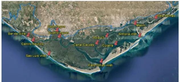
In this study, the data used are the data that was collected by MaréFormosa project in which consists of time series data of water level and velocity (longitudinal component) variations, in several locations in Ria Formosa, covering complete tidal cycle. These data were taken from 12 stations in the main channel of Ria Formosa (Fig 4.1) and were measured in normal meteorological condition which means it is not affected by the wind, storm, and rain. The identified stations were limited in the west and central part of Ria Formosa lagoon. Those are Cais centro nautico, Bar da gina, Poita Nave Pegos, Quatro Aguas, Sao luis inlet, Faro-Olhao inlet, Canal Cacoes, Culatra, Boia V3, Armona inlet, Marim, and Bela Romao. The Bela Romao station was considered as a reference control of Fuzeta inlet in the eastern part of Ria Formosa, due to its significant role in Ria Formosa lagoon. The coordinate location of each stations can be seen from Table 4.1.
Fig 4.1. Tides parameter locations which are currently being measured by MareFORMOSA
project, in Ria Formosa (red pins).
The current and water column pressure/depth were taken by using ADP (Aquadopp Current Profiler) of NORTEK. The pressure range of ADP piezoresistive (pressure sensor) is about 0-100 m with the accuracy of 0.25%, while the velocity range is about 10 m/s horizontal and 5 m/s along beam with 1% accuracy of measured value ±0.5 cm/s. ADP measures current at 0.5 m interval starting from 0.4 m above the head of ADP equipment. The height of the installed equipment is 0.8 m from bottom.
Table 4.1. Coordinate location of the stations
stations x (UTM) y (UTM)
Barra Faro-Olhão 23380.87 -299044
Armona inlet 29290.71 -295059
Barra S Luís 15564.26 -297957
Cais Centro Náutico 13102.33 -295835
Bar da Gina 12309.32 -295100 Esteiro Cações 22787.09 -296264 Boia V3 24307.06 -295167 Culatra 25659.83 -296369 Marim 28678.3 -293269 Bela Romão 31924.71 -292305 Quatro Águas 17077.1 -295254
Estaleiro Nave Pegos 46ENP 16709.33 -294315
Beside ADP, the pressure transducer level TROLL 300 and TROLL 700 were also used to measure the water level variation. The pressure transducer level TROLL 300 has the accuracy value of ± 0.01% FS with non vented range 30-300 psia, while pressure transducer level TROLL 700 has the accuracy value of ± 0.005% FS with non vented range of 30-500 psia and vented range of 5-500 psig.
Due to the limitation of ADP equipment, the measurements using ADP in each stations were conducted in different time. The ADP measurements were measured during short period of time. By using Pressure transducer equipment which installed in Faro Olhao inlet as a reference control point of the water level measurement in Ria Formosa lagoon, the long time series of water level variation for 2 years were measured.
The short period of time measurement using ADP in each stations were adjusted with the pressure transducer long time series of water level measurement in Faro Olhao inlet. Then from this time adjustment, the similar tidal height and tidal period measurement which measured in Faro Olhao inlet in those each short time series were chosen and the date occurrence of them were recorded (Table 4.2). Based on the recorded date, the ADP velocity and water level measurements for each stations were filtered. Hence, each stations has adjusted time series data of water level and longitudinal component of velocity variations. The tidal height and tidal period measurement for each stations can be seen in Table 4.2.
All data which are taken should be calibrated with the local atmospheric variation and hydrographic zero (Portuguese datum), which is negative for the value below the hydrographic zero and positive for the value above the hydrographic zero.
Table 4.2. The tidal height (H) and tidal period (T) of the tide in each stations (TP measurement) No code station Tidal Height (m) Phase Period (hour) Tidal Period (T) (hour) Occurrence Flood Ebb Flood Ebb
1 1 Faro-‐Olhao inlet -‐2.32 2.24 6.5 5.42 11.92 3/6/2011 4:15 2 5 Armona inlet -‐2.34 2.32 6.42 5.83 12.25 11/9/2011 2:45 3 6 Culatra -‐2.34 2.31 6.42 6.08 12.5 15/10/2011 4:45 4 7 Boia V3 -‐2.34 2.29 6.67 5.5 12.17 24/10/2011 1:10 5 8 Marim -‐2.29 2.32 6.42 5.75 12.17 10/11/2011 14:10 6 9 Canal Cacoes -‐2.32 2.27 6.58 5.58 12.17 12/12/2011 15:45 7 11 Bela Romao -‐2.29 2.26 6.75 5.83 12.58 15/1/2012 6:30 8 17 Sao Luis inlet -‐2.32 2.21 6.42 5.83 12.25 24/5/2012 16:30 9 19 Centro Nautica -‐2.37 2.21 6.33 5.75 12.08 8/7/2012 6:35 10 20 Bar de Gina -‐2.28 2.24 6.33 5.75 12.08 31/7/2012 1:55 11 22 Quatro Aguas -‐2.24 2.21 6.5 5.67 12.17 28/11/2012 14:25 12 25 Poita Nave Pegos -‐2.3 2.2 6.42 5.5 11.92 12/5/2013 3:45
AVERAGE -‐2.31 2.26 6.48 5.71 12.19 STANDAR DEVIATION 0.03 0.05 0.13 0.18 0.20 RANGE OF STD 0.07 0.09 0.26 0.37 0.39
4.2. Data Treatment
All the calculations are conducted during mid tide (in between Neap and Spring tide).
4.2.1. Raw Time Series
Time series data of water level and longitudinal component of velocity variations for complete tidal cycle were used. For each time series, the spatial water level gradient (barotropic pressure gradient) is determined by calculating the difference between water level of the two/three close adjacent stations for every stations in the main channel of Ria Formosa, and so does for the longitudinal/spatial velocity gradient.
4.2.2. Harmonic Analysis
Harmonic Analysis methods was used to obtain the best fit between the raw data and the harmonic constituent combination/superposition curve for all stations. The harmonic constituent that are taken into account are M2 and M4, since they are the most dominant tidal
constituent in Ria Formosa (Dias and Sousa, 2009a), besides S2. The tidal constituent of S2 was not taken into account in this study because the tidal period of data used in this study is less than 24 hours. The harmonic analysis of time series computes a least squares solution fitting the input time series with currents and water level variation of input periods according
Godin, 1972 in Foreman & Henry (1989). The harmonic analysis script was written by Brian O. Blanton (Skidaway Institute of Oceanography USA - Fall 1996) and modified by Duarte N. R. Duarte (University of Algarve - Spring 2008) to allow data gaps.
4.2.2.1. Tidal distortion / Tidal asymmetry
The effect of frictional distortion of the tidal curve is also considered in terms of production of the M4, M6 over tides from the M2 tide. The major part of the asymmetry of the
tide curve can be represented by superposition of M2 and M4, both in terms of height and
velocity. ) 2 cos( ) cos( 2 4 4 2 M M M M t a t a A=
ω
−θ
+ω
−θ
) 2 cos( ) cos( 2 4 4 2 M M M M t u t u u=ω
−ϕ
+ω
−ϕ
Where a and θ are the amplitude and phase of tidal height, and u and φ are the amplitude and phase of the tidal velocity. The elevation phase of M4 relative to M2 is
4 2 4
2 2
2M −M = θM −θM .The elevation amplitude ratio is M4/M2 =aM4/aM2. Speer and
Aubrey (1985) in Dyer (1997) have considered the implications of these ratios and show that for an elevation phase (2M2-M4) between 0 and 180o the system will be flood dominant, and
for a phase of 180o - 360o it will be ebb dominant. In either case the larger the M4/ M2ratio, the more distorted and the more strongly flood or ebb dominated the system becomes. Thus the dominance can be predicted from tidal analysis (Dyer, 1997).
The flood/ebb dominance is also determined from tidal current velocities. If the ebb velocity is larger than flood velocity, then it is ebb dominance (Dias et al., 2009b). The result that obtained from the tidal current analysis then is compared with the result that obtained from the tidal height analysis.
4.2.2.2. Energy Flux and Dissipation
To calculate the energy flux along an estuarine channel, the equation can be written as follow (Pugh, 1987) : U gh P ρ η 2 1 = [W m-1]
h is the undisturbed water depth along the channel, (ɳ) is the amplitude of the water level, and (U) is the amplitude of the axial tidal current, ρ is water density, and g is gravity.
Dissipation energy along the channel can be reached by dividing energy flux (P) by the distance L separating the two stations, or can be written as follow:
L P P
D=[ n+1− n]/ [W m-2]
Where n is a station counter. By dividing the equation of dissipation energy (D) above with h and ρ yields the dissipation in W kg-1.
An alternate estimate of tidal energy dissipation at each station can be done using the following equation (Taylor, 1919) :
> =< 2 3 2] [U C D ρ d
Where the bracket pair <> represent the average over the M2 cycle, Cd is a drag coefficient and U is the tidal velocity.
4.2.2.3. Error Calculation
Error estimation can be calculated using elevation and velocity root mean square errors as follows:
∑
= − = nt i i i e nt RMS 1 2 ) ~ ( 1 η η And{
}
∑
= − + − = nt i i i i i v u u v v nt RMS 1 2 2 ( ~) ) ~ ( 1Where ɳ is the amplitude of elevation, u and v are the amplitude of depth-averaged velocities, the tilde represents numerical results, nt is the number of time step (Fortunato et al., 1997).
4.2.3. Hysteresis Diagram Analysis
To calculate the phase lags and slack water between water level (ɳ) and velocity (v), a graphic time series of vertical component (water level) and graphic time series of horizontal component (longitudinal component of velocity) for each stations are established. These two graphics are combined in order to create hysteresis diagram analysis for all tidal cycles. Hysteresis diagram is created for standing tidal wave as an open ellipse and progressive wave as a line and also for the combination of the two types (Dyer, 1997). The progressive wave contribution can be estimated by measuring the time difference between high and low water and slack water. This can then be expressed as a proportion of the tidal period in degrees or in hour (Dyer, 1997).
4.2.4. GIS Application
In this study, Arc GIS platform was used to determine the cross section profile for each stations which will be used to calculate the hydraulic geometrical parameters for each stations. Besides that, Arc GIS was used also to perform the spatial distribution of water level gradient, velocity gradient, volume, and residence time, and to compare the volume that goes in and out through the inlet (inlet tidal cycle volume) with the annual critical geometry volume of the lagoon which based on the water level variation during high water and low water.
4.2.4.1. Hydraulic Geometrical Parameters Calculation
Hydraulic geometrical parameters that were calculated are cross-section area (Aɳ,t),
wet perimeter (Pɳ,t), surface width (Lsɳ,t), mean depth (hɳ,t) and hydraulic radius (Rhɳ,t). The
calculations are conducted for each stations and for each time (hourly).
To calculate the mean depth (h) and hydraulic radius (Rh). the equations below can be used : t t t Ls A h , , , η η η = and t t t h P A R , , , η η η =
4.2.4.2. Spatial Distribution Performance
4.2.4.2.1. The mean velocity (ūn,t) in the water column
To calculate the mean velocity in the water column (ūn,t) for each stations and time,
the integration velocity method in the water column (per linear meter) can be used. The equation can be defined as follow :
∫
⋅ = h z t n u dz h u 0 , 1Where uz is the velocity at z meter, z is the distance from the bottom, and h is the depth of the
flow that are obtained from ADP (Acoustic Doppler Current Profiler).
Since the ADP measured the uz value several meters above the beds, the interpolation
technique to calculate the uz value from bed till those several meters were addressed. To
calculate those uz value, the bed shear velocity (u*) and the roughness coefficient (zo) were
determined using graphical method (open university, 2000). The equation of this graphical method can be defined as follow:
756 . 5 / _ _ _
* slope of the graph
) _ _ _ ) _ _ _ (int (
10 ercepton on y axis slope of the graph
o
z = −
Then uz value on the water column can be calculated using Von Karman-Prandtl
universal equation as follow: ⎟⎟⎠ ⎞ ⎜⎜⎝ ⎛ = o z z z u u *ln ) ( κ
where κ is von karman coefficient (κ=0.41).
4.2.4.2.2. The mean velocity in the channel cross section (<ūn,t>)
When only one velocity profile was obtained at the middle of channel cross-section, Manning model can be used to calculate the velocities for the entire cross section (<ūn,t>) for
each stations and time, considering constant on the cross-section the roughness Manning coefficient Cm and null the transverse energy gradient (∂E∂y). The manning model equation can be expressed as follows:
2 1 3 2 , 1 E R C u h m t n >= ⋅ ⋅ < 3 2 3 2 , , h R u u h t n t n > = <
When E represents the energy gradient of the flow; <ūn,t> is the mean velocity on the
channel cross section; ūn,t is the mean velocity obtained on the middle point of the cross
section; Rh is the hydraulic radius of the cross section, and h is the depth of the channel (or
the mean depth h). So to calculate the mean velocity in the channel cross section, it is assumed that the manning coefficient (Cm) in the cross section is constant, and also the energy gradient in the cross section.
4.2.4.2.3. The mean velocity in the channel cross section during flood and ebb (<ūn>flood
and <ūn>ebb)
During flood and ebb period, the mean velocity in the channel cross section for each stations were determined by summing the mean velocity in the channel cross section during flood period for mean flood velocity and during ebb period for mean ebb velocity. The equations can be written as follows :
l Mean Flood Velocity :
flood t n t t t flood n T dt u u flood ⋅ > < = > <
∫
= =0l Mean Ebb Velocity : ebb t n t t t ebb n T dt u u ebb ⋅ > < = > <
∫
= =0 4.2.4.2.4. Net VelocityAfter calculated all calculation above, net velocity, flood and ebb mean velocity, and residual velocity can be calculated.
l Net velocity = <ūn>flood - <ūn>ebb
4.2.4.2.5. Water Discharge (Qn) and water volume (Vn)
The water discharge/flow of water is expressed in units of volume per time. In flow measurement, flow is often estimated by determining the velocity at which water flows through a given cross-sectional area, known as general continuity equation, which defines as follows: t t n u A Q nt , _ , =< , >× η
Then, the flooding and ebbing time must be determined to calculate the discharge and volume during the flood and ebb phase, using equation below:
dt A u Q flood t n flood t t t t t n ⎟⋅ ⎠ ⎞ ⎜ ⎝ ⎛< >× =
∫
=0= , _ , , η and∫
= = ⎟⎠⋅ ⎞ ⎜ ⎝ ⎛< >× = ebb t n ebb t t t t t n u A dt Q 0 , _ , , ηWater volume for each stations during flood and ebb can be calculated using the equation as follows:
flood f
f Q t
V = × and Ve =Qe×tebb
4.2.4.2.6. Residence Time (RT) calculation
The residence time (RT) is the average duration for a water molecule to pass through a subsystem of the hydrologic cycle (Chow et al., 1988) or the time required for a particle to travel from a location to the boundary of the region (Wang et al., 2004). To calculate the residence time for each stations (station 1, station 2, station 3, etc), the equation below (Sanford et al., 1992 inside Wang et al., 2004) can be used :
RT P b T P V RT time residence + − + = ) 1 ( ) 2 / ( ) ( _
Where V is low tide volume of the whole or a segment of the estuary, P is tidal prism, T is tidal period, b is return flow factor, and R is river discharge.
Tidal prism is equal to volume of ocean water coming into an estuary on the flood tide + volume of river discharge mixing with that ocean water. This simple equation below can be used : river from in flood in V V P prism Tidal_ ( )= _ + _ _
Return flow can be define as the ratio of the difference between the outflowing ebb velocity and the incoming flood velocity (Moore et al., 2006). To calculate the return flow factor (b), the equation below can be used :
U U b M M + − = 2 2 υ υ
Where ʋM2 is the vertically averaged amplitude of the M2 tidal harmonic over the period for
which the slope was determined and U is the vertically averaged axial velocity (tides removed), which can be obtained using equation as follows (Moore et al., 2006):
x gh U Cd ∂ ∂ − = η 2
Where Cd is drag coefficient, g is the acceleration gravity, h is the mean depth of the cross section at the mouth of estuary, and dɳ/dx is the average water level slope along the axis.
To obtain drag coefficient Cd, the equation below (Soulsby, 1997) can be used :
2 u Cd o =ρ⋅ ⋅ τ
( )
2 * u o=ρ⋅ τOr other Cd equation below could also be used (Bricker, J.D. Et al, 2005) :
2 0 100 2 0 100 ln ln ⎟⎟ ⎟ ⎟ ⎠ ⎞ ⎜⎜ ⎜ ⎜ ⎝ ⎛ ⎟⎠ ⎞ ⎜⎝ ⎛ = → ⎟⎟ ⎟ ⎟ ⎠ ⎞ ⎜⎜ ⎜ ⎜ ⎝ ⎛ ⎟⎠ ⎞ ⎜⎝ ⎛ = z C z z Cd κ κ .
Where zo is the zero velocity level on the depth profile (u=0 m/s at z=zo) or roughness
coefficient, κ is von karman-prandtl coefficient, ρ is water density, τo is bed shear stress, uis
the depth averaged current velocity, and u* is shear velocity.
4.2.4.2.7. GIS performance
After calculating the residence time in each stations, the spatial residence time variation can be shown using interpolation method of IDW (Inverse Distance Weight) in GIS software using radius setting of 4 points and distance of 4000 m. To determine and evaluate the suitable area for shellfish pond, the average current velocity, maximum flood current, and